A queueing theory approach for a multi-speed exclusion process.

Abstract

We consider a one-dimensional stochastic reaction-diffusion generalizing the totally asymmetric simple exclusion process, and aiming at describing single lane roads with vehicles that can change speed. To each particle is associated a jump rate, and the particular dynamics that we choose (based on 3-sites patterns) ensures that clusters of occupied sites are of uniform jump rate. When this model is set on a circle or an infinite line, classical arguments allow to map it to a linear network of queues (a zero-range process in theoretical physics parlance) with exponential service times, but with a twist: the service rate remains constant during a busy period, but can change at renewal events. We use the tools of queueing theory to compute the fundamental diagram of the traffic, and show the effects of a condensation mechanism.

1 A multi-speed exclusion process

The totally asymmetric exclusion process (tasep) is a popular statistical physics model of one-dimensional interacting particles particularly adapted to traffic modeling. This is due to its simple definition, and to the non-trivial exact solutions which have been unveiled in the stationary regime DeEvHaPa . One important shortcoming of this model is that it does not allow particles to move at different speeds. Cellular automata like the Nagel-Schreckenberg model NaSch address this issue, leading to very realistic though still simple simulators. However, these models are difficult to handle mathematically beyond the mean field approximation ChSaSc and an approximate mapping with the asymmetric chipping model suggests that the jamming phenomenon takes place as a broad crossover rather than a phase transition LeZi . In this paper, we are interested in analyzing the nature of fluctuations in the fundamental diagram (fd), that is the mean flow of vehicles plotted against the traffic density. To address this question, we propose to extend the tasep in a different way, more convenient for the analysis albeit less realistic from the point of view of traffic.

Figure 1: The basic $1$-dimensional tasep model.

The elementary $1$-dimensional tasep (Fig. 1) model is defined on a discrete lattice (e.g. a finite ring with boundary periodic conditions, a segment with edges or an infinite line), where each site may be occupied with at most one particle. Each particle moves independently to the next site (say, to the right), at the times of a Poisson process with intensity $\mu$. Therefore, the model is a continuous time Markov process, which state is the binary encoded sequence $\sigma_{t}\in\{O,V\}^{N}$ of size $N$ (the size of the system), where the letter $V$ (resp. $O$) denotes a vehicle (resp. an empty space) at site $i$. Each transition involves two consecutive letters when a particle moves from site $i$ to site $i+1$:

$$VO\ \operatorname*{\rightarrow}^{\mu}\ OV.$$

Figure 2: The multi-speed $1$-dimensional tasep model.

In order to encode various speed levels, we propose to extend the basic tasep by allowing the particle to jump at different possible rates which themselves vary stochastically in time (Fig. 2). Assuming for now a finite number of $n-1$ speed levels, the Markov chain that we consider is a sequence encoded into a $n$-alphabet $\{O,A,B,\ldots\}$

$$\sigma_{t}=\{V_{i},\ldots,i=1\ldots N\},\qquad V_{i}\in\{O,A,B,\ldots\}$$

where $O$ is again an empty site, and $A$, $B,\ldots$ represent occupied sites with jump rates $\mu_{a},\mu_{b},\ldots$. In our model, the transitions remain local: the particle may jump to the next site only if it is empty, we allow the final state to be conditioned by the site after the next. More precisely, we assume that any transition involves three consecutive letters, and distinguish between two cases:

$$\begin{cases}\displaystyle\ldots XOY\ldots\operatorname*{\rightarrow}^{\mu_{x}}\ldots OYY\ldots,\qquad Y\neq O\qquad\text{rule 1,}\\[5.69046pt] \displaystyle\ldots XOO\ldots\operatorname*{\rightarrow}^{\mu_{x}}\ldots OZO\ldots,\qquad Z\neq O\qquad\text{rule 2.}\end{cases}$$

In the second case, the type (or equivalently the jump rate) of the particle is chosen randomly according to a distribution $F$. As a limiting case, we will consider a general continuous distribution $F$ on $\mathbb{R}^{+}$. In other words, a particle at site $i$ with rate $\mu_{x}$ jumps to site $i+1$ and acquires a new rate $\mu_{z}$ which is a random function of $V_{i+2}$.

The basic assumption is that if a car gets in close contact to another one, it will adopt its rate. Conversely, if it arrives at a site not in contact with any other car, the new rate will be freely determined according to some random distribution. This models the acceleration or deceleration process in an admittedly crude manner. This setting is different from usual exclusion processes with multi-type particles, each having its own jump rate. It is more in line with the Nagel-Schreckenberg model, with the difference that only local jumps are allowed and speed is replaced by jump rate.

2 $L$-stage tandem queue reformulation

In the context of exclusion processes, jams are represented as cluster of particles. Clustering phenomena can be analyzed in some cases by mapping the process to a tandem queueing network (i.e. a zero range processes in statistical physics terms). For the simple tasep on a ring two dual mappings are possible:

• the queues are associated to empty sites and the clients are the particles in contact behind this site,

• the queues are associated with particles and the clients are the empty sites in front of this particle.

By using one of these mappings, the tasep is equivalent to a closed cyclic queueing network, with fixed service rates equal to the jumping rate $\mu$ of the particles. Steady states of such queueing network have been analyzed thoroughly (see for ex. Kelly Kel ) in terms of a simple product form structure which we expose now.

Consider an open $L$-stage tandem queue, with arrival rate $\lambda$ and a common service rate $\mu$: $L$ queues with service rate $\mu$ are arranged in successive order (the departures from a given queue coincide with the arrivals to the next one) and the arrival process of the first queue is Poisson with intensity $\lambda$. Each queue is stable when $\lambda<\mu$, transient when $\lambda>\mu$. It is then well known that the distribution of the number of clients $X_{1},\ldots,X_{L}$ in the queues is

$$P(\{X_{i}=x_{i},i=1\ldots L\})=\prod_{i=1}^{L}P_{\lambda}(X_{i}=x_{i}),$$ (1)

where

$$P_{\lambda}(X_{i}=x)=(1-\rho)\rho^{x},\qquad\text{with}\qquad\rho\stackrel{{\scriptstyle\mbox{\tiny def}}}{{=}}\frac{\lambda}{\mu}.$$

If the network is closed (the last queue is connected to the first one in the ring geometry), then expression (1) remains valid, with the constraint that the total number of clients $\sum_{i=1}^{L}X_{i}$ is fixed. In this case, $\lambda$ can be chosen arbitrarily, as long as each queue in isolation remains ergodic.

It can be shown easily PuMe that, for a plain tasep on a ring, the size of the jams is asymptotically a geometric random variable with parameter $\rho$ (when $N=kL$, $k=1,2\ldots$). In the open geometry, the arrival rate is an external parameter which can be set between $0$ and $\mu$. When it becomes comparable to the service rate, i.e. when $\rho\simeq 1$, large queues may form and a random walk first time return calculation yields a realistic scaling behavior for the lifetime distribution of jams NaPa

$$P(t)\simeq t^{-3/2}.$$

Figure 3: Mapping of the variable-speed tasep to a tandem queue

In our multi-speed exclusion process, particles are guaranteed by construction to form clusters with homogeneous speed, and the mapping of empty sites to queues is suitable (Fig. 3). The new feature is that the service rate $R_{i}$ of a given queue can change with time: it is drawn randomly from a distribution with cumulative distribution $F$ when the first customer arrives. It is assumed that there exists a minimal service rate $\mu_{0}>0$ such that $F(\mu_{0})=0$. $\rho_{0}=\lambda/\mu_{0}\leq 1$ is therefore the maximal possible load. The state is determined by the pair $(X,R)$ and the possible transitions are as follows:

$$(X=x,R=\mu) \xrightarrow{\lambda\leavevmode\hbox{\rm\small 1\kern-3.15005pt\normalsize 1}_{\{x>0\}}}(X=x+1,R=\mu),$$

$$(X=0,R=\mu) \xrightarrow{\lambda F(d\mu^{\prime})}(X=1,R=\mu^{\prime}),$$

$$(X=x,R=\mu) \xrightarrow{\mu\leavevmode\hbox{\rm\small 1\kern-3.15005pt\normalsize 1}_{\{x>0\}}}(X=x-1,R=\mu).$$

Figure 4: State graph for isolated queues in the case of (a) the multi-speed process definition, and (b) a non-reversible queue with hysteresis. States are represented by black dots and transitions by arrows.

Since these transitions form a tree (see Fig. 4(a)), each queue in isolation is a reversible Markov process and its stationary distribution reads:

$$P_{\lambda}(X=x,R\in d\mu)=P_{\lambda}(X=0)F(d\mu)\left(\frac{\lambda}{\mu}\right)^{x},$$

with

$$P_{\lambda}(X=0)=\left(\int_{\mu_{0}}^{\infty}F(d\mu)\frac{\mu}{\mu-\lambda}\right)^{-1}.$$

The distribution of the number of customers in the queue is therefore no longer geometric:

$$P_{\lambda}(X=x)=\int_{\mu_{0}}^{\infty}P_{\lambda}(X=x,R\in d\mu)=P_{\lambda}(X=0)\int_{\mu_{0}}^{\infty}F(d\mu)\left(\frac{\lambda}{\mu}\right)^{x}.$$ (2)

Nevertheless, the product form expression (1) for the invariant measure remains valid, because of the reversibility of the individual queues taken in isolation (see again Kel ). The stationary distribution of the $L$-stage tandem queue takes the form

$$P_{\lambda}(S)=\prod_{i=1}^{L}P_{\lambda}(X_{i},R_{i}),$$

for any sequence $S=\{(X_{i},R_{i}),i=1,\ldots,L\}$. While each queue has a different service rate at a given time, all the queues have globally the same distribution. Our model is therefore encoded in the single queue stationary distribution $P_{\lambda}(X_{i},R_{i})$.

3 The fundamental diagram

As announced in Section 1, we turn now to the fundamental diagram (fd), that is the plot of the mean flow of vehicles against the traffic density. By nature, the fluctuations in the fd are associated to the jam formation. Schematically, three main distinct regimes or traffic phases have been identified by empirical studies Kerner : one for to free-flow, and two congested states, the “synchronized flow” and the “wide moving jam”.

In the case of the basic tasep, it is well known, and rigorously proved in some cases, that an hydrodynamic limit can be obtained by rescaling both the spatial variable $x=i/N$ and the jumping rate according to $\mu(N)=NV_{0}$, where $N$ is a rescaling which we let to $\infty$ and $V_{0}$ is a constant. The corresponding coarse grained density $\rho$ satisfies the inviscid Burger equation

$$\frac{\partial\rho}{\partial t}=V_{0}\frac{\partial}{\partial x}\Bigl{[}\rho(1-\rho)\Bigr{]}.$$

The fd at this scale is deterministic, since

$$J(\rho)=V_{0}\rho(1-\rho),$$

and symmetric w.r.t. $\rho=1/2$ because of the particle-hole symmetry. $V_{0}$ represents the free velocity of cars, when the density is very low.

In practice, points plotted in experimental fd studies are obtained by averaging data from static loop detectors over a few minutes (see e.g. Kerner ). This is difficult to do with our queue-based model, for which a space average is much easier to obtain. The equivalence between time and space averaging is not an obvious assumption, but since jams are moving, space and time correlations are combined in some way NaPa and we consider this assumption to be quite safe. In what follows, we will therefore compute the fd by considering either the joint probability measure $P_{\lambda}(d,\phi)$ for an open system, or the conditional probability measure $P_{\lambda}(\phi|d)$ for a closed system, where

$$\begin{cases}\displaystyle d=\frac{N}{N+L},\\[5.69046pt] \displaystyle\phi=\frac{\Phi}{N+L},\end{cases}\ \text{with}\ \begin{cases}L&\text{number of queues}\\ \displaystyle N=\sum_{i=1}^{L}X_{i}&\text{number of vehicles}\\[5.69046pt] \displaystyle\Phi=\sum_{i=1}^{L}R_{i}\leavevmode\hbox{\rm\small 1\kern-3.15005pt\normalsize 1}_{\{X_{i}>0\}}&\text{integrated flow}\end{cases}$$

are spatial averaged quantities and represent respectively the density and the traffic flow. We perform the analysis in the ring geometry: this avoids edge effects, fixes the numbers $N$ of vehicles and $L$ of queues, and finally makes sense as an experimental setting. In the statistical physics parlance, the fact that $N$ is fixed means that we are working with the canonical ensemble. As a result this constraint yields the following form of the joint probability measure:

$$P(S)=\frac{1}{Z_{L}[N]}\prod_{i=1}^{L}P_{\lambda}(x_{i},\mu_{i}),$$

with the canonical partition function

$$Z_{L}[N]\stackrel{{\scriptstyle\mbox{\tiny def}}}{{=}}\sum_{\{x_{i}\}}\prod_{i=1}^{L}P_{\lambda}(x_{i})\delta\bigl{(}\textstyle N-\sum_{i=1}^{L}x_{i}\bigr{)}.$$

These expressions are actually independent of $\lambda$ in this specific ring geometry. The density-flow conditional probability distribution takes the form

$$P(\phi|d)=\frac{Z_{L}[N,\Phi]}{Z_{L}[N]},$$ (3)

with

$$N=\frac{d}{1-d}L,\qquad\Phi=\frac{\phi}{1-d}L,$$

and

$$Z_{L}[N,\Phi]\stackrel{{\scriptstyle\mbox{\tiny def}}}{{=}}\sum_{\{x_{i}\}}\int\!\!\cdots\!\!\int\prod_{i=1}^{L}P_{\lambda}(x_{i},d\mu_{i})\textstyle\delta\bigl{(}N-\sum_{i=1}^{L}x_{i}\bigr{)}\delta\bigl{(}\Phi-\sum_{i=1}^{L}\mu_{i}\leavevmode\hbox{\rm\small 1\kern-3.15005pt\normalsize 1}_{\{x_{i}>0\}}\bigr{)}.$$ (4)

Note (by simple inspection, see e.g. Kel ) that $P(\phi|d)$ is independent of $\lambda$.

4 Phase transition and condensation mechanism

The connection between spontaneous formation of jams and the Bose-Einstein condensation has been analyzed in some specific models, with e.g. quenched disorder Evans , where particles are distinguishable with different but fixed hopping rates attached to them. In the present situation, all particles are identical, but hopping rates may fluctuate, which is related to annealed disorder in statistical physics. The condensation mechanism for zero range processes within the canonical ensemble has been clarified in some recent work EvMaZi . Let us translate in our settings the main features of the condensation mechanism. Assume that the number of clients $X$ of an isolated queue has a long-tailed distribution

$$P(X=x)\operatorname*{\propto}_{x\gg 1}\frac{1}{x^{\alpha}},\quad\alpha>1.$$

The empirical mean queue size reads

$$\bar{X}=\frac{1}{L}\sum_{i=1}^{L}X_{i},\qquad\text{and}\qquad\mathbb{E}\bar{X}=\mathbb{E}_{\lambda}(X)\stackrel{{\scriptstyle\mbox{\tiny def}}}{{=}}\frac{\int_{\mu_{0}}^{\infty}F(d\mu)\frac{\lambda\mu}{(\mu-\lambda)^{2}}}{\int_{\mu_{0}}^{\infty}F(d\mu)\frac{\mu}{\mu-\lambda}},$$

where $\mathbb{E}_{\lambda}(X)$ is the expected number of clients in an isolated queue, when the arrival rate is $\lambda$. Within the canonical ensemble, $\bar{X}$ is fixed, while for the grand canonical ensemble, only the expectation $\mathbb{E}(\bar{X})$ is fixed. In both cases, for $\alpha>2$ there exists $\bar{X}_{c}$ such that, when $\bar{X}>\bar{X}_{c}$ ($\mathbb{E}(\bar{X})>\bar{X}_{c}$ in the grand canonical ensemble), one of the queues condenses, i.e. carries a macroscopic number of particles. When $\alpha>2$, there is a condensate with probability weight $O(L^{1-\alpha})$.

This condensation corresponds to a second order phase transition, and occurs at a critical density $d_{c}$ which is the same in the canonical and grand-canonical formalism. To determine $d_{c}$, first consider

$$\bar{d}(\lambda)\stackrel{{\scriptstyle\mbox{\tiny def}}}{{=}}\frac{\mathbb{E}_{\lambda}(X)}{1+\mathbb{E}_{\lambda}(X)}.$$

$\mathbb{E}_{\lambda}(X)$ increases monotonically with $\lambda$, which cannot exceed $\mu_{0}$ (see Section 2). Therefore, if $\mathbb{E}_{\mu_{0}}(X)\ =\ x_{c}\ <\ \infty$, then there exists a critical density

$$d_{c}=\frac{x_{c}}{1+x_{c}},$$

such that for $d\geq d_{c}$ one of the queues condenses. The interpretation is that $N_{c}=Lx_{c}$ is the maximal number of clients that can be in the queues in the fluid regime, and the less costly way to absorb the excess $N-N_{c}$ is to put it in one single queue. Let us give an example, by specifying the joint law through

$$P(\mu_{0}\leq R\leq\mu_{0}y)=F(\mu_{0}y)=\Bigl{(}\frac{y-1}{r-1}\Bigr{)}^{\alpha},\qquad 1\leq y\leq r,$$ (5)

where $r>1$ is ratio between the highest and lowest speed. In that case, using (2) we have the following asymptotic as $\xi\to\infty$

$$P_{\lambda}(X=x)\propto\ \Bigl{(}\frac{\lambda}{\mu_{0}}\Bigr{)}^{x}\int_{1}^{r}(y-1)^{\alpha-1}y^{-x}dy\sim\frac{1}{x^{\alpha}}\Bigl{(}\frac{\lambda}{\mu_{0}}\Bigr{)}^{x},$$

and $\mathbb{E}_{\mu_{0}}(X)<\infty$ when $\alpha>2$, which yields the possibility of condensation above the critical density

$$d_{c}(\alpha,r)=\frac{(r-1)^{\alpha-2}}{\alpha-2+(r-1)^{\alpha-2}}.$$ (6)

5 Numerical results

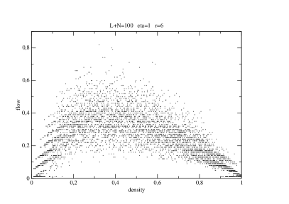
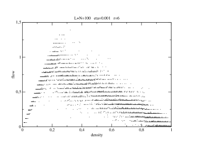
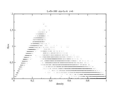
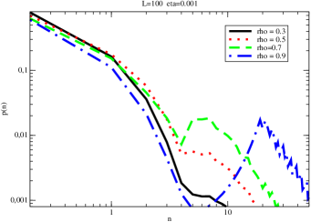
Figure 5: Probabilistic fundamental diagram on the ring geometry ($L+N=100$) for a two-level speed distribution with $\eta=1$ (a), $0.001$ (b) and $10^{-6}$ (c); corresponding single queue distribution as a function of the density for $\eta=0.001$ (d).

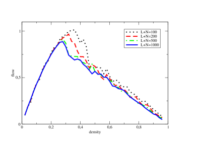
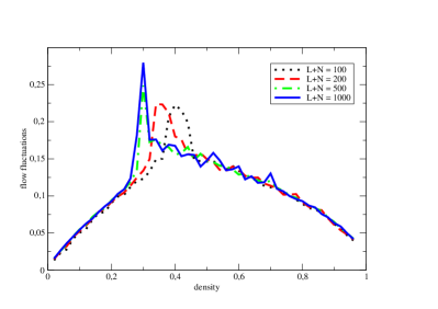
Figure 6: Mean flow as a function of density for a continuous speed distribution ($\alpha=3$) on the ring geometry with varying sizes $L+N$ (left) and corresponding standard deviation rescaled by $\sqrt{L}$ (right).

The analysis of (3) in the ring geometry can in principle be performed by means of saddle point techniques EvMaZi ; FaLa , which we postpone to another work. Instead we present a numerical approach: the fd presented in Fig. 5(a)-(c) is obtained by solving the recursive relation

$$Z_{L}[N,\Phi]=P_{\lambda}(X=0)Z_{L-1}[N,\Phi]+\sum_{x=1}^{N}\int P_{\lambda}(x,d\mu)Z_{L-1}[N-x,\Phi-\mu\leavevmode\hbox{\rm\small 1\kern-3.15005pt\normalsize 1}_{\{x>0\}}],$$

up to some value $L_{MAX}=100$ for the number of queues, with a fixed value of $\lambda<\mu_{0}$. Although in principle one arbitrary value of $\lambda$ should suffice, in practice, the results for different values of $\lambda$ have to be superposed in the diagram to get significant results. Since this recursion is only tractable with a finite number of possible velocities, the distribution $F$ used here is concentrated to two values $\mu_{0}$ and $\mu_{1}$. The presence of a discontinuity in the fundamental diagram for small values of $\eta\stackrel{{\scriptstyle\mbox{\tiny def}}}{{=}}P(R=\mu_{0})/P(R=\mu_{1})$ is a finite size effect, which disappears when the system size is increased while $\eta$ is kept fixed. Nevertheless, the direct simulation of the closed $L$-stage tandem queues, with continuous distribution (5), indicates as expected a second order phase transition when $\alpha>2$ (Fig. 6). This transition is related to the formation of a condensate, which is marked by the apparition of a bump in the single queue distribution at the critical density (see Fig. 5(d)). This condensation mechanism is responsible for the slope discontinuity. Fluctuations scale like $1/\sqrt{L}$, as expected from the Central Limit Theorem. Note however that the critical density is different than the one given by (6) for the open system.

6 Perspectives

In this work, we analyze the fluctuations in the fundamental diagram of traffic by considering models from statistical physics and using probabilistic tools. We propose a generalization of the tasep by considering a multi-speed exclusion process which is conveniently mapped onto an $L$-stage tandem queue. When the individual queues are reversible, general results from queueing network theory let us obtain the exact form of the steady state distribution. This measure is conveniently shaped to compute the fd. Depending on the speed distribution, it may present two phases, the free-flow and the congested ones, separated by a second order phase transition. This transition is associated to a condensation mechanism, when slow clusters are sufficiently rare.

In practice, it is conjectured Kerner that there are three phases in the fd, separated by first order phase transition. A large number of possible extensions of our model are possible, by playing with the definition of the state graph of a single queue (Fig. 4(a)). This graph accounts either for the dynamics of single vehicle clusters, when queues are associated to empty sites, or to the behavior of single drivers when queues are associated to occupied sites. In order to obtain first order phase transitions, we will consider in future work models where the single queues are not reversible in isolation, for example because of an hysteresis phenomenon (Fig. 4(b)).

References

- (1) B. Derrida, M. R. Evans, V. Hakim, and V. Pasquier. Exact solution for 1d asymmetric exclusion model using a matrix formulation. J. Phys. A: Math. Gen., 26:1493–1517, 1993.
- (2) K. Nagel and M. Schreckenberg. A cellular automaton model for freeway traffic. J. Phys. I,2, pages 2221–2229, 1992.
- (3) D. Chowdhury, L. Santen, and A. Schadschneider. Statistical physics of vehicular traffic and some related systems. Physics Report, 329:199, 2000.
- (4) E. Levine, G. Ziv, L. Gray, and D. Mukamel. Phase transitions in traffic models. J. Stat. Phys., 117:819–830, 2004.
- (5) F. P. Kelly. Reversibility and stochastic networks. John Wiley & Sons Ltd., 1979. Wiley Series in Probability and Mathematical Statistics.
- (6) O. Pulkkinen and J. Merikoski. Cluster size distributions in particle systems with asymmetric dynamics. Physical Review E, 64(5):56114, 2001.
- (7) K. Nagel and M. Paczuski. Emergent traffic jams. Phys. Rev. E, 51(4):2909–2918, 1995.
- (8) B. S. Kerner. Experimental features of self-organization in traffic flow. Phys. Rev. Lett., 81(17):3797–3800, 1998.
- (9) M. R. Evans. Bose-einstein condensation in disordered exclusion models and relation to traffic flow. Europhys. Lett, 36(1):13–18, 1996.
- (10) M. R. Evans, S. N. Majumdar, and R. K. P. Zia. Canonical analysis of condensation in factorized steady states. Journal of Statistical Physics, 123(2):357–390, 2006.
- (11) G. Fayolle and J.-M. Lasgouttes. Asymptotics and scalings for large closed product-form networks via the Central Limit Theorem. Markov Proc. Rel. Fields, 2(2):317–348, 1996.