The 2XMMi/SDSS Galaxy Cluster Survey

We present a catalogue of X-ray selected galaxy clusters and groups as a first release of the 2XMMi/SDSS Galaxy Cluster Survey. The survey is a search for galaxy clusters detected serendipitously in observations with XMM-Newton in the footprint of the Sloan Digital Sky Survey (SDSS). The main aims of the survey are to identify new X-ray galaxy clusters, investigate their X-ray scaling relations, identify distant cluster candidates, and study the correlation of the X-ray and optical properties. In this paper, we describe the basic strategy to identify and characterize the X-ray cluster candidates that currently comprise 1180 objects selected from the second XMM-Newton serendipitous source catalogue (2XMMi-DR3). Cross-correlation of the initial catalogue with recently published optically selected SDSS galaxy cluster catalogues yields photometric redshifts for 275 objects. Of these, 182 clusters have at least one member with a spectroscopic redshift from existing public data (SDSS-DR8). We developed an automated method to reprocess the XMM-Newton X-ray observations, determine the optimum source extraction radius, generate source and background spectra, and derive the temperatures and luminosities of the optically confirmed clusters. Here we present the X-ray properties of the first cluster sample, which comprises 175 clusters, among which 139 objects are new X-ray discoveries while the others were previously known as X-ray sources. For each cluster, the catalogue provides: two identifiers, coordinates, temperature, flux [0.5-2] keV, luminosity [0.5-2] keV extracted from an optimum aperture, bolometric luminosity $L_{500}$, total mass $M_{500}$, radius $R_{500}$, and the optical properties of the counterpart. The first cluster sample from the survey covers a wide range of redshifts from 0.09 to 0.61, bolometric luminosities $L_{500}=1.9\times 10^{42}-1.2\times 10^{45}$ erg s^-1, and masses $M_{500}=2.3\times 10^{13}-4.9\times 10^{14}$ M_⊙. We extend the relation between the X-ray bolometric luminosity $L_{500}$ and the X-ray temperature towards significantly lower $T$ and $L$ and still find that the slope of the linear $L-T$ relation is consistent with values published for high luminosities.

1 Introduction

Galaxy clusters are the most visible tracers of large-scale structure. They occupy very massive dark matter halos and are observationally accessible by a wide range of means. Their locations are found to corresponding to large numbers of tightly clustered galaxies, pools of hot X-ray emitting gas, and relatively strong features in the gravitational lensing shear field. Precise observations of large numbers of clusters provide an important tool for testing our understanding of cosmology and structure formation. Clusters are also interesting laboratories for the study of galaxy evolution under the influence of extreme environments (Koester et al., 2007).

The baryonic matter of the clusters is found in two forms: first, individual galaxies within the cluster, which are most effectively studied through optical and NIR photometric and spectroscopic surveys; and second, a hot, ionized intra-cluster medium (ICM), which can be studied by means of its X-ray emission and the Sunyaev-Zeldovich (SZ) effect (Sunyaev & Zeldovich, 1972, 1980). The detection of clusters using SZ effect is a fairly new and highly promising technique for which tremendous progress has been made in finding high redshift clusters and measuring the total cluster mass (e.g. Planck collaboration et al., 2011; Vanderlinde et al., 2010; Marriage et al., 2010).

The X-ray selection of clusters has several advantages for cosmological surveys: the observable X-ray luminosity and temperature of a cluster is tightly correlated with its total mass, which is indeed its most fundamental parameter (Reiprich & Böhringer, 2002). These relations provide the ability to measure both the mass function (Böhringer et al., 2002) and power spectrum (Schuecker et al., 2003), which directly probe the cosmological models. Since the cluster X-ray emission is strongly peaked on the dense cluster core, X-ray selection is less affected by projection effects than optical surveys and clusters can be identified efficiently over a wide redshift range.

Many clusters have been found in X-ray observations with Uhuru, HEAO-1, Ariel-V, Einstein, and EXOSAT, which have allowed a more accurate characterization of their physical proprieties (for a review, see Rosati et al. (2002)). The ROSAT All Sky Survey (RASS, Voges et al., 1999) and the deep pointed observations have led to the discovery of hundreds of clusters. In ROSAT observations, 1743 clusters have been identified, which are compiled in a meta-catalogue called MCXC by Piffaretti et al. (2010). The MCXC catalogue is based on published RASS-based (NORAS, REFLEEX, BCS, SGP, NEP, MACS, and CIZA) and serendipitous (160D, 400D, SHARC, WARPS, and EMSS) cluster catalogues.

The current generation of X-ray satellites XMM-Newton, Chandra, and Suzaku have provided follow-up observations of statistical samples of ROSAT clusters for cosmological studies (Vikhlinin et al., 2009) and detailed information on the structural proprieties of the cluster population (e.g. Vikhlinin et al., 2006; Pratt et al., 2010; Arnaud et al., 2010). Several projects are ongoing to detect new clusters of galaxies from XMM-Newton and Chandra observations (e.g. the XSC (Romer et al., 2001), XDCP (Fassbender et al., 2007), XMM-LSS (Pierre et al., 2006), COSMOS (Finoguenov et al., 2007), SXDS (Finoguenov et al., 2010), and ChaMP (Barkhouse et al., 2006)).

In this paper, we present the 2XMMi/SDSS galaxy cluster survey, a search for galaxy clusters based on extended sources in the 2XMMi catalogue (Watson et al., 2009) in the field of view the Sloan Digital Sky Survey (SDSS). The main aim of the survey is to build a large catalogue of new X-ray clusters in the sky coverage of SDSS. The catalogue will allow us to investigate the correlation between the X-ray and optical properties of the clusters. One of the long term goals of the project is to improve the X-ray scaling relations, and to prepare for the eROSITA cluster surveys, a mid term goal is the selection of the cluster candidates beyond the SDSS-limit for studies of the distant universe. Here we present a first cluster sample of the survey which comprises 175 clusters found by cross-matching the 2XMMi sample with published SDSS based optical cluster catalogues.

The paper is organized as follows: in Sect. 2 we describe the procedure of selecting the X-ray cluster candidates as well as their possible counterparts in SDSS data. In Sect. 3 we describe the X-ray data the reduction and analysis of the optically confirmed clusters. The discussion of the results is described in Sect. 4. Section 5 concludes the paper. The cosmological parameters $\Omega_{\rm M}=0.3$, $\Omega_{\Lambda}=0.7$ and $H_{0}=70$ km s^-1 Mpc^-1 were used throughout this paper.

2 Sample construction

We describe our basic strategy for identifying clusters among the extended X-ray sources in the 2XMMi catalogue. We then proceed by cross-matching the initial catalogue with those of optically selected galaxy clusters from the SDSS thus deriving a catalogue of X-ray selected and optically confirmed clusters with measured redshifts, whose X-ray properties are analysed in Sect. 3.

2.1 X-ray cluster candidate list

X-ray observations provide a robust method for the initial identification of galaxy clusters as extended X-ray sources. A strategy to create a clean galaxy cluster sample is to construct a catalogue of X-ray cluster candidates followed by optical observations. XMM-Newton archival observations provide the basis for creating catalogues of serendipitously identified point-like and extended X-ray sources. The largest X-ray source catalogue ever produced is the second XMM-Newton source catalogue (Watson et al., 2009). The latest edition of this catalogue is 2XMMi-DR3, which was released on 2010 April 28. The 2XMMi-DR3 covers 504 deg² and contains $\sim 3$ times as many discrete sources as either the ROSAT survey or pointed catalogues. The catalogue contains 353191 X-ray source detections corresponding to 262902 unique X-ray sources detected in 4953 XMM-Newton EPIC (European Photon Imaging Camera) observations made between 2000 February 3 and 2009 October 8.

The 2XMMi-DR3 contains 30470 extended source detections, which form the primary database for our study. This initial sample contains a very significant number of spurious detections caused by the clustering of unresolved point sources, edge effects, the shape of the PSF (point spread function) of the X-ray mirrors, large extended sources consisting of several minor sources, and other effects such as X-ray ghosts and similar.

We applied several selection steps to obtain a number of X-ray extended sources that were then visually inspected individually. In our study, we considered only sources at high Galactic latitudes, $|b|>20\degr$, and discarded those that were flagged as spurious in the 2XMMi-DR3 catalogue by the screeners of the XMM-Newton SSC (Survey Science Centre). The source detection pipeline used for the creation of the 2XMMi catalogues allows for a maximum core radius of extended sources of 80 arcsec. Sources with extent parameters equalling that boundary were discarded, screening of a few examples shows that those sources are spurious or large extended sources (the targets of the observations) that were discarded anyhow. This initial selection reduced the number to 4027 detections.

Since our main aim is the generation of a serendipitous cluster sample, we removed sources that were the targets of the XMM-Newton observation. We also discarded fields containing large extended sources and selected only those fields within the footprint of SDSS, which left 1818 detections. After removing multiple detections of the same extended sources (phenomena caused by either problematic source geometries in a single XMM-Newton observation or duplicate detections in a re-observed field), the catalogue was reduced to 1520 extended sources that were regarded as unique.

This list still contains spurious detections for a number of reasons: (a) point-source confusion, (b) resolution of one asymmetric extended source into several symmetric extended sources, (c) the ill-known shape of the PSF leads to an excess of sources near bright point-sources, for both point-like and extended sources, and (d) edge effects/low exposure times. To remove the obvious spurious cases, we visually inspected the X-ray images of the initial 1520 detections using the FLIX upper limit server. As a result, we were left with 1240 confirmed extended X-ray sources.

We then made use of the SDSS to remove additional non-cluster sources. We downloaded the XMM-Newton EPIC X-ray images from the XMM-Newton Science Archive (XSA: Arviset et al., 2002) and created summed EPIC (PN+MOS1+MOS2) images in the energy band $0.2-4.5$ keV. Using these, we created smoothed X-ray contours, which were overlaid onto co-added $r$, $i$, and $z-$band SDSS images. Visual inspection of those optical multi-colour images with X-ray contours overlaid, allowed us to remove extended sources corresponding to nearby field galaxies, as well as those objects that are likely spurious detections. The resulting list which passes these selection criteria contains 1180 cluster candidates, about 75 percent of which are newly discovered.

Figure 1 shows the X-ray-optical overlay of a new X-ray cluster, which has a counterpart in SDSS at photometric redshift = 0.4975 and a stellar mass centre indicated by the cross-hair as given by Szabo et al. (2011) (see Section 2.2). We use this cluster to illustrate the main steps of our analysis in the following sections. In Appendix A, Figures A.1 to A.4 show the X-ray-optical overlays and the extracted X-ray spectra for four clusters illustrating results for various redshifts covered by our sample and different X-ray fluxes.

Figure 1: The X-ray-optical overlay of the representative cluster 2XMM J104421.8+213029 at photometric redshift = 0.4975. The X-ray contours are overlaid on the SDSS co-added image obtained in $r$, $i$, and $z$-bands. The field of view is $4^{\prime}\times 4^{\prime}$ centred on the X-ray cluster position. The cross-hair indicates the cluster stellar mass centre as given by Szabo et al. (2011).

About one quarter of the X-ray selected cluster candidates have no plausible optical counterpart. These are regarded as high-redshift candidates beyond the SDSS limit at $z\geq 0.6$, and suitable targets for dedicated optical/near-infrared follow-up observations (see e.g.  Lamer et al., 2008).

2.2 The cross-matching with optical cluster catalogues

The SDSS offers the opportunity to produce large galaxy-cluster catalogues. Several techniques were applied to identify likely clusters from multiband imaging and SDSS spectroscopy. We use those published catalogues to cross-identify common sources in our X-ray selected and those optical samples. All these optical catalogues give redshift information per cluster, which we use in the following to study the X-ray properties of our sources ($z_{p}$ indicates a photometric, $z_{s}$ a spectroscopic redshift).

Table 1 lists the main properties of the optical cluster catalogues that we used to confirm our X-ray selection. Below we provide a very brief description of each of these together with the acronym used by us:

• GMBCG The Gaussian Mixture Brightest Cluster Galaxy catalogue (Hao et al., 2010) consists of more than 55,000 rich clusters across the redshift range $0.1<z_{p}<0.55$ identified in SDSS-DR7. The galaxy clusters were detected by identifying the cluster red-sequence plus a brightest cluster galaxy (BCG). The cross-identification of X-ray cluster candidates with the GMBCG within a radius of 1 arcmin yields 136 confirmed clusters.

• WHL The catalogue of Wen, Han & Liu (Wen et al., 2009) consists of 39,668 clusters of galaxies drawn from SDSS-DR6 and covers the redshift range $0.05<z_{p}<0.6$. A cluster was identified if more than eight member galaxies of $M_{r}\leq–21$ were found within a radius of 0.5 Mpc and within a photometric redshift interval $z_{p}\pm 0.04(1+z_{p})$. We confirm 150 X-ray clusters by cross-matching within 1 arcmin.

• MaxBCG The max Brightest Cluster Galaxy catalogue (Koester et al., 2007) lists 13,823 clusters in the redshift range $0.1<z_{p}<0.3$ from SDSS-DR5. The clusters were identified using maxBCG red-sequence technique, which uses the clustering of galaxies on the sky, in both magnitude and colour, to identify groups and clusters of bright E/S0 red-sequence galaxies. The cross-match with our X-ray cluster candidate list reveals 54 clusters in common within a radius of one arcmin.

• AMF The Adaptive Matched Filter catalogue of Szabo et al. (2011) lists 69,173 likely galaxy clusters in the redshift range $0.045<z_{p}<0.78$ extracted from SDSS-DR6 using an adaptive matched filter (AMF) cluster finder. The cross-match yields 127 confirmed X-ray galaxy clusters.

In the AMF-catalogue, the cluster centre is given as the anticipated centre of the stellar mass of the cluster, while in the other three catalogues the cluster centre is the position of the brightest galaxy cluster (BCG).

Many of our X-ray selected clusters have counterparts in several optical cluster catalogues within our chosen search radius of one arcmin. In these cases, we use the redshift of the optical counterpart, which has minimum spatial offset from the X-ray position. Table1 lists in the second to last column the number of matching X-ray sources per optical catalog individually and in the last column the final number after removal of duplicate identifications.

The unique optically confirmed X-ray cluster sample obtained by cross-matching with the four catalogues consists of 275 objects having at least photometric redshifts.

Table 1: Main properties of the cluster catalogues with optically (SDSS-based) selected entries. The last two columns give the number of matching X-ray selected clusters individually and cumulatively.

CLG	Nr.	Redshift	SDSS	X-ray	Nr.CLG
catalogue	CLG	range		CLG ($1^{\prime}$)	sample
GMBCG	55,000	0.1 - 0.55	DR7	136	123
WHL	39,688	0.05 - 0.6	DR6	150	72
MaxBCG	13,823	0.1 - 0.3	DR5	54	20
AMF	69,173	0.045 - 0.78	DR6	127	60
Total					275

After cross-identification, we found 120 clusters of the optically confirmed cluster sample with a spectroscopic redshift for the brightest galaxy cluster (BCG) from the published optical catalogues. Since the latest data release, SDSS DR8, provides more spectroscopic redshifts, we searched for additional spectra of BCGs and other member galaxies. We ran SDSS queries searching for galaxies with spectroscopic redshifts $z_{s(g)}$ within 1 Mpc from the X-ray centre. We considered a galaxy as a member of a cluster if $|z_{p}-z_{s(g)}|<0.05$.

The spectroscopic redshift of the cluster was calculated as the average redshift for the cluster galaxies with spectroscopic redshifts. The confirmed cluster sample with spectroscopic redshifts for at least one galaxy includes 182 objects. Therefore, the unique optically confirmed X-ray cluster sample has the photometric redshifts for all of them, 120 spectroscopic redshifts for 120 BCGs from the optical cluster catalogues, and 182 clusters with one or more members with spectroscopic redshifts from the SDSS database. Figure 2 shows the distribution of the cluster photometric redshift $z_{p}$, the distribution of spectroscopic redshifts $z_{s}$ of the BCGs as given in the various optical cluster catalogues, and the average spectroscopic redshift of the cluster members (which we refer to as the cluster spectroscopic redshift) for the confirmed cluster sample. Figure 3 shows the distribution of the number of cluster galaxies that have a spectroscopic redshift in the SDSS database. The relation between the photometric and spectroscopic redshifts of the cluster sample is shown in Figure 4. Since this relation was found to be tight (where the Gaussian distribution of ($z_{s}$ - $z_{p}$) has $\sigma$ = 0.02), we were able to rely on the photometric redshifts for the cluster with no spectroscopic information.

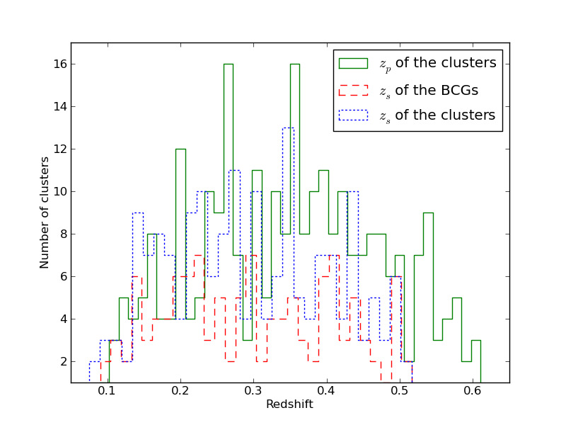
Figure 2: The distribution of the optical redshifts for the confirmed clusters sample. The distribution includes the cluster photometric redshifts $z_{p}$ (solid line) with a median 0.36, spectroscopic redshifts of the BCGs $z_{s}$ (dashed line) with a median 0.3 from the optical cluster catalogues and the cluster spectroscopic redshifts $z_{s}$ (dotted line) with a median 0.3 from the SDSS data.

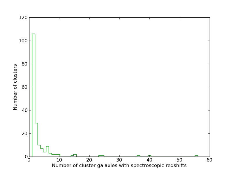
Figure 3: The distribution of the spectroscopically confirmed cluster members per cluster.

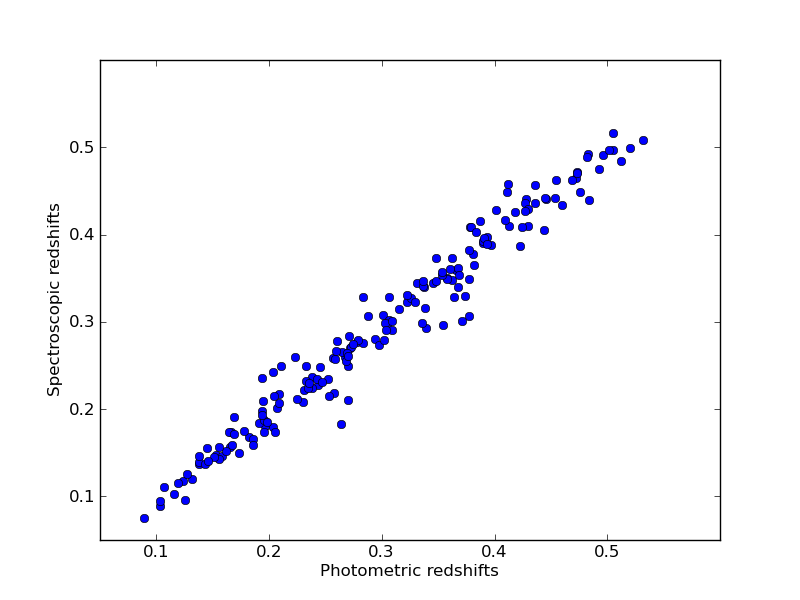
Figure 4: The relation between the photometric and spectroscopic redshifts of the confirmed cluster sample.

We used an angular separation of one arcmin to cross-match the X-ray cluster candidates with the optical cluster catalogues. The corresponding linear separation was calculated using the spectroscopic redshift, if available, or the photometric redshift. Figure 5 shows the distribution of the linear separation between the X-ray centre and the BCG position. For AMF clusters (60 objects), we identified the BCGs of 40 systems within one arcmin and computed their offsets, which are included in this aforementioned distribution. The BCGs were selected as the brightest galaxies with $|z_{p}-z_{p(BCG\ cand.)}|<0.05$ among the three BCG candidates given for each AMF cluster published by Szabo et al. (2011). The other 20 AMF clusters are not included in Fig. 5, because their BCG is outside one arcmin. It is not always the case that the BCG lies exactly on the X-ray peak. Rykoff et al. (2008) model the optical/X-ray offset distribution by matching a sample of maxBCG clusters to known X-ray sources from the ROSAT survey. They found a large excess of X-ray clusters associated with the optical cluster centre. There is a tight core in which the BCG is within $\sim$ 150 h^-1 kpc of any X-ray source, as well as a long tail extending to $\sim$ 1500 h^-1 kpc. It is shown in Figure 5 that the majority of the confirmed sample have the BCG within a radius ($\sim$ 150 kpc), as well as a tail extending to 352 kpc that is consistent with the optical/X-ray offset distribution of Rykoff et al. (2008).

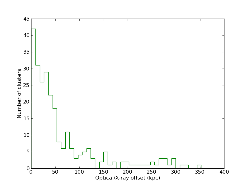
Figure 5: The distribution of the linear separation between the position of the BCG and the X-ray cluster position.

We searched the Astronomical Database SIMBAD and the NASA/IPAC Extragalactic Database (NED) to check whether they had been identified and catalogued previously. We used a search radius of one arcmin. About 85 percent of the confirmed sample are new X-ray clusters, while the remainder had been previously studied using ROSAT, Chandra, or XMM-Newton data.

3 X-ray data analysis

The optically confirmed clusters have a wide range of source counts (EPIC counts in the broad band energy 0.2-12 keV from the 2XMMi-DR3 catalogue) from 66 to 28000 counts as shown in Figure 6. To analyse the X-ray data, we have to determine the optical redshifts, except for some candidates with more than 1000 net photons for which it is possible to estimate the X-ray redshift (e.g. Lamer et al., 2008; Yu et al., 2011). In this paper, we use the cluster spectroscopic redshifts where available or the photometric redshifts that we obtained from the cross-matching as described in the previous section.

The data reduction and analysis of the optically confirmed sample was carried out using the XMM-Newton Science Analysis Software (SAS) version 10.0.0.

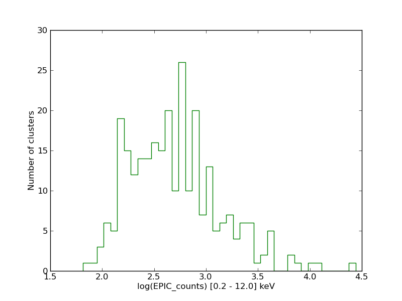
Figure 6: The distribution of EPIC counts in [0.2-12] keV as given in the 2XMMi-DR3 catalogue for the confirmed cluster sample.

3.1 Standard pipelines

The raw XMM-Newton data were downloaded using the Archive InterOperability System (AIO), which provides access to the XMM-Newton Science Archive (XSA). The raw data were provided in the form of a bundle of files known as observation data files (ODF), which contain uncalibrated event files, satellite attitude files, and calibration information. The main steps in the data reduction were: (i) the generation of calibrated event lists for the EPIC (MOS1, MOS2, and PN) cameras using the latest calibration data. This was done using the SAS packages cifbuild, odfingest, epchain, and emchain. (ii) The creation of background light curves to identify time intervals with poor quality data. (iii) The filtering of the EPIC event lists to exclude periods of high background flaring and bad events. (iv) To create a sky image of the filtered data set. The last three steps were performed using SAS packages evselect, tabgtigen, and xmmselect.

3.2 Analysis of the sample

We now describe the procedure to determine the source and background regions for each cluster, extract the source and background spectra, fit the X-ray spectra, and finally measure the X-ray parameters (e.g. temperature, flux, and luminosity). As input to the task generating the X-ray spectra, we used the filtered event lists as described in the previous section.

3.2.1 Optimum source extraction radius

The most critical step in generating the cluster X-ray spectra is to determine the source extraction radius. We developed a method to optimize the signal-to-noise ratio (SNR) of the spectrum for each cluster. To calculate the extraction radius with the highest integrated SNR we created radial profiles of each cluster in the energy band $0.5-2.0$ keV. Background sources, taken from the EPIC PPS source lists, were excluded and the profiles were exposure corrected using the EPIC exposure maps. Since we did not perform a new source detection run, the SNR was calculated as a function of radius taking into account the background levels as given in the 2XMMi catalogue.

The radial profiles of the X-ray surface brightness of the representative cluster in MOS1, MOS2 and PN data are shown in Fig. 7. The background values of the cluster in the EPIC images are indicated by the horizontal line with the same colours as the profiles. Figure 8 shows the SNR profiles of the representative cluster in MOS1, MOS2, PN and EPIC (MOS1+MOS2+PN) data as a function of the radius from the cluster centre. The optimum extraction radius ($72^{\prime\prime}$) is determined from the maximum value in the EPIC SNR plot, which is indicated by a point in Fig. 8.

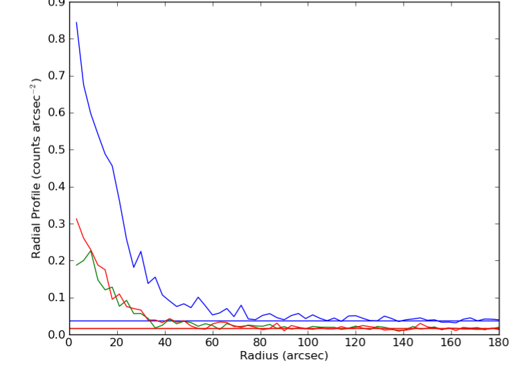
Figure 7: The radial profile of 2XMM J104421.8+213029 MOS1(green), MOS2(red), and PN (blue) images. The horizontal lines indicate the background values for MOS1, MOS2 and PN with the same colour as the profile.

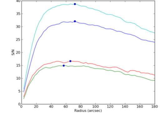
Figure 8: The signal-to-noise ratio (SNR) profiles of 2XMM J104421.8+213029 in MOS1 (green), MOS2 (red), PN (blue) and EPIC (MOS1+MOS2+PN) (cyan) data. The cluster optimum extraction radius ($72^{\prime\prime}$) is corresponding to the highest SNR as indicated by a point in the EPIC SNR profile.

3.2.2 Spectral extraction

The EPIC filtered event lists were used to extract the X-ray spectra of the cross-correlated X-ray optical cluster sample. The spectra of each cluster candidate were extracted from a region with an optimum extraction radius as described in the previous section. The background spectra were extracted from a circular annulus around the cluster with inner and outer radii equalling two and three times the optimum radius, respectively. Other unrelated nearby sources were masked and excluded from the source and background regions that were finally used to extract the X-ray spectra. Figure 9 shows the cluster and background regions, as well as the excluded regions of field sources for the representative cluster. The SAS task especget was used to generate the cluster and background spectra and to create the response matrix files (redistribution matrix file (RMF) and ancillary response file (ARF)) required to perform the X-ray spectral fitting with XSPEC.

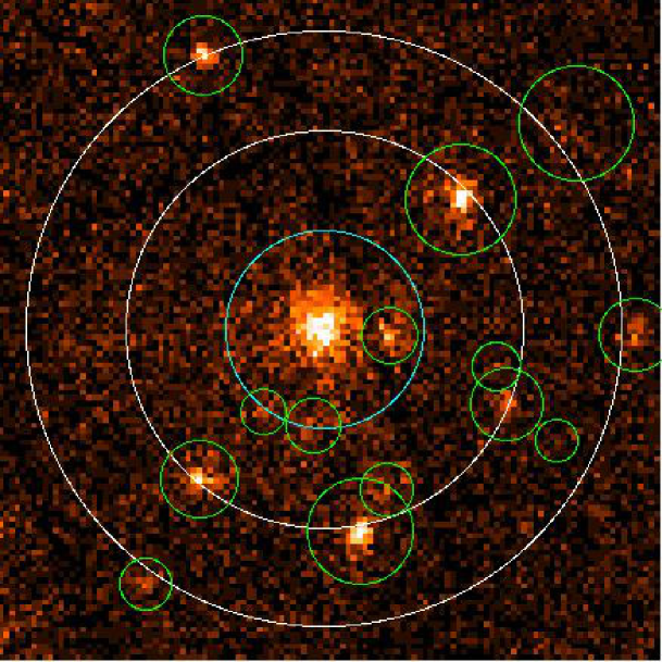
Figure 9: The representative cluster extraction region is the inner circle with colour cyan. The background region is the annulus with white colour. The excluding field sources are indicated by green circles. The field of view is $8^{\prime}\times 8^{\prime}$ centred at the cluster position.

3.2.3 Spectral fitting

The photon counts of each cluster spectrum were grouped into bins with at least one count per bin before a fit of a spectral model was applied to the data using the Ftools task grppha. The spectral fitting was carried out using XSPEC software version 12.5.1 (Arnaud, 1996). Before executing the algorithm to fit the spectra, the Galactic HI column (nH) was derived from the HI map from the Leiden/Argentine/Bonn (LAB) survey (Kalberla et al., 2005). This parameter was fixed while fitting the X-ray spectrum. The redshift of the spectral model was fixed to the optical cluster redshift either the spectroscopic redshift for 182 clusters or the photometric redshift for the remainder cluster sample.

For each cluster, the available EPIC spectra were fitted simultaneously. The employed fitting model was a multiplication of a $\tt TBABS$ absorption model (Wilms et al., 2000) and a single-temperature optically thin thermal plasma component (the $\tt MEKAL$ code in XSPEC terminology, Mewe et al., 1986) to model the X-ray plasma emission from the ICM. The metallicity was fixed at 0.4 $Z\odot$. This value is the mean of the metallicities of 95 galaxy clusters in the redshift range from 0.1 to 0.6 (the same redshift range of the confirmed sample) observed by Chandra (Maughan et al., 2008). The free parameters are the X-ray temperature and the spectral normalization. The fitting was done using the Cash statistic with one count per bin following the recommendation of Krumpe et al. (2008) for small count statistics.

To avoid the fitting algorithm converging to a local minimum of the fitting statistics, we ran series of fits stepping from 0.1 to 15 keV with a step size = 0.05 using the $\tt{steppar}$ command within XSPEC. The cluster temperature, its flux in the [0.5-2] keV band, its X-ray luminosity in the [0.5-2] keV band, the bolometric luminosity, and the corresponding errors were derived from the best-fitting model. We assumed that the fractional error in the bolometric luminosity was the same as the fractional error in the aperture luminosity [0.5-2] keV (within an aperture defined by the optimum extraction radius). Figure 10 shows the fits to the EPIC (MOS1, MOS2, and PN) spectra and the models for the representative cluster. Figures A.1 to A.4 in the Appendix A show the fitted spectra of four clusters with different X-ray surface brightnesses and data qualities at different redshifts covering the whole redshift range of the confirmed clusters.

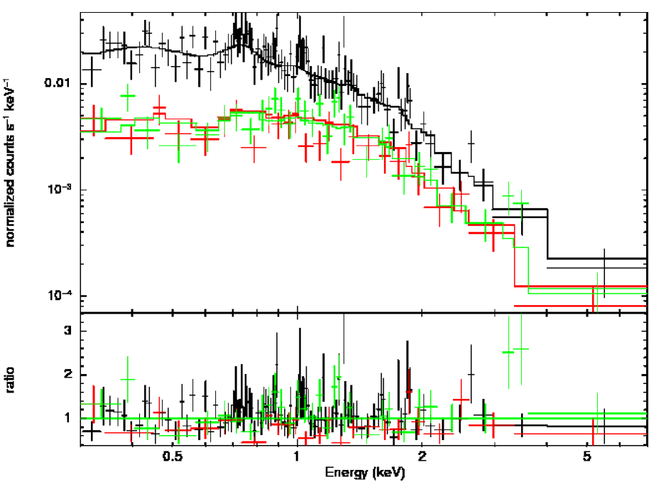
Figure 10: The EPIC PN (black), MOS1 (green) and MOS2 (red) data with the best-fit MEKAL model for the representative cluster.

4 Analysis of a cluster sample with reliable X-ray parameters

We analysed the X-ray data of the optically and X-ray confirmed clusters to measure the average temperature of the hot ICM. We developed an optimal extraction method for the X-ray spectra maximising the SNR. The cluster spectra were fitted with absorbed thin thermal plasma emission models with pre-determined redshift and interstellar column density to determine the aperture X-ray temperature ($T_{ap}$), flux ($F_{ap}$) [0.5-2] keV, luminosity ($L_{ap}$) [0.5-2] keV, and their errors. We accepted the measurements of $T_{ap}$ and $L_{ap}$ if the fractional errors were smaller than 0.5. About 80 percent of the confirmed clusters passed this fractional error filter. For these clusters, another visual screening of the spectral fits (Figure 10) and the X-ray images (Figure 9) was done. When the spectral extraction of a given cluster was strongly affected by the exclusion of field sources within the extraction radius or a poor determination of the background spectrum, it was also excluded from the final sample, which comprises 175 clusters. For a fraction of 80 percent, this is the first X-ray detection and the first temperature measurement.

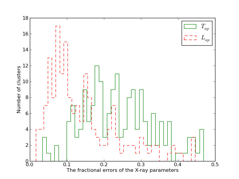
Figure 11: The distribution of the fractional errors in the X-ray temperatures (solid) and luminosities (dashed) derived from spectra extracted within the optimum aperture for the energy range 0.5-2 keV of the first cluster sample.

Our subsequent presentation of our analysis and discussion refers to those 175 objects with reliable X-ray parameters. The distribution of the $T_{ap}$ and $L_{ap}$ [0.5-2] keV fractional errors for the first cluster sample is shown in Fig. 11. It is clearly evident that the cluster luminosity is more tightly constrained than the temperature. For about 86 percent of the sample, the fractional errors are smaller than 0.25. Therefore, we estimated several physical parameters for each cluster based on the bolometric luminosity $L_{bol}$ within the optimal aperture. The median correction factor between aperture bolometric luminosities and aperture luminosities in the energy band [0.5-2] keV ( $L_{bol}$ / $L_{ap}$ ) was found to be 1.7. We assumed that the fractional error in $L_{bol}$ was identical to that of $L_{ap}$ [0.5-2] keV. The estimated parameters are $R_{500}$ the radius at which the mean mass density is 500 times the critical density of the Universe (see Eq. 2) at the cluster redshift, $L_{500}$ the bolometric luminosity within $R_{500}$, and $M_{500}$ the cluster mass within $R_{500}$. We used an iterative procedure to estimate the physical parameters using published $L_{500}-T_{500}$ and $L_{500}-M_{500}$ relations (Pratt et al., 2009, their orthogonal fit for $M_{500}$ with Malmquist bias correction). Our procedure is similar to that used by Piffaretti et al. (2010) and Šuhada et al. (2010), which consists of the following steps:

• We estimate $M_{500}$ using the $L-M$ relation

  $$M_{500}=2\times 10^{14}M_{\odot}\ \bigl{(}\frac{h(z)^{-7/3}\ L_{bol}}{1.38\times 10^{44}\ erg\ s^{-1}}\Bigr{)}^{1/2.08},$$ (1)

  where $h(z)$ is the Hubble constant normalised to its present-day value, $h(z)=\bigl{[}\Omega_{\rm M}(1+z)^{3}+\Omega_{\Lambda}\Bigr{]}^{1/2}$. We approximate $L_{500}$ as the aperture bolometric luminosity $L_{bol}$, which we correct in an iterative way.

• We compute $R_{500}$

  $$R_{500}=\sqrt[3]{3M_{500}/4\pi 500\rho_{c}(z)},$$ (2)

  where the critical density is $\rho_{c}(z)=h(z)^{2}3H^{2}/8\pi G$ .

• We compute the cluster temperature within $R_{500}$ using the $L-T$ relation

  $$T=5\mbox{keV}\ \bigl{(}\frac{h(z)^{-1}\ L_{bol}}{7.13\times 10^{44}\ erg\ s^{-1}}\Bigr{)}^{1/3.35}.$$ (3)

• We calculate the core radius $r_{core}$ and $\beta$ using scaling relations from Finoguenov et al. (2007)

  $$r_{core}=0.07\times R_{500}\times\bigl{(}\frac{T}{1\ keV}\bigr{)}^{0.63},$$ (4)

  $$\beta=0.4\ \bigl{(}\frac{T}{1\ keV}\bigr{)}^{1/3}.$$ (5)

• We calculate the enclosed flux within $R_{500}$ and the optimum aperture by extrapolating the $\beta$-model. The ratio of the two fluxes is calculated, i.e. $\gamma=F_{500}/F_{\rm bol}$.

• We finally compute a corrected value of $L_{500}=\gamma\times L_{\rm bol}$.

We then considered $L_{500}$ as input for another iteration and all computed parameters were updated. We repeated this iterative procedure until converging to a final solution. At this stage, the $L_{500}$, $M_{500}$, and $R_{500}$ were determined. The median correction factor between extrapolated luminosities and aperture bolometric luminosities ($L_{500}$/$L_{\rm bol}$) was 1.5. To calculate the errors in Eqs. 1 and 3, we included the measurement errors in the aperture bolometric luminosity $L_{bol}$ , the intrinsic scatter in the $L-T$ and $L-M$ relations, and the propagated errors caused by the uncertainty in their slopes and intercepts. For Eq. 4 and Eq. 5, we included only the propagated errors of their independent parameters since their intrinsic scatter had not been published. Finally, all the measured errors were taken into account when computing the errors in $L_{500}$ and $M_{500}$ in the last iteration. The errors in $L_{500}$ and $M_{500}$ were still underestimated because of the possible scatter in the relations in Eq. 4 and Eq. 5.

We investigated the $L-T$ relation in the first cluster sample using $T_{ap}$ and $L_{500}$. Figure 12 shows the relation between $L_{500}$ (corrected for the redshift evolution) and $T_{ap}$ (uncorrected for cooling flows). Here we assumed that $T_{ap}$ did not differ significantly from $T_{500}$ and its error was derived from the spectral fits. The best-fit linear relation (solid line) derived from an orthogonal distance regression fit (ODR) (Boggs & Rogers, 1990, which takes into account measurement errors in both variables) between their logarithm, is

$$\log\ (h(z)^{-1}\ L_{500})=(0.57\pm 0.05)+(3.41\pm 0.15)\ \log\ (T_{ap}).$$ (6)

The best-fit power law relation derived from a BCES orthogonal fit to the $L_{500}$ - $T_{500}$ relation published by Pratt et al. (2009) for the REXCESS sample is plotted as the dashed line in Fig. 12. The ODR slope (present work), $3.41\pm 0.15$, is consistent with the BCES orthogonal slope (Pratt et al., 2009) of the REXCESS sample, $3.35\pm 0.32$. In addition, the present slope is consistent with the BCES orthogonal slope (3.63 $\pm$ 0.27) of the $L-T$ relation derived from a sample of 114 clusters (without excluding the core regions) observed with Chandra across a wide range of temperature (2 $<$ kT $<$ 16 keV) and redshift (0.1 $<$ z $<$ 1.3) by Maughan et al. (2011).

We tested the corresponding uncertainty in the error budget of $L_{500}$ caused by the above-mentioned unknown scatter in Eq. 4 and 5: for example, a $\sigma=\pm 0.1$ scatter in the $\beta$ value results in a fractional error in $L_{500}$ of 17$\%$. If we take into account the newly estimated errors in $L_{500}$ when fitting the $L-T$ relation, the revised slope of 3.32 is within the error in the original slope as in Eq. 6 and still consistent with the published ones.

Our sample represents cluster temperatures ranging from 0.45 to 5.92 keV and values of bolometric luminosity in the $L_{500}$ range $1.9\times 10^{42}-1.2\times 10^{45}$ erg s^-1 in a wide redshift range 0.1 - 0.6. Most of the published $L-T$ relations were derived from local cluster samples with temperatures higher than 2 keV. The current relation is derived for our sample, which includes clusters and groups with low temperatures and luminosities in a wide redshift range up to $z=0.6$. The distribution of luminosity as a function of redshift is shown in Fig. 13.

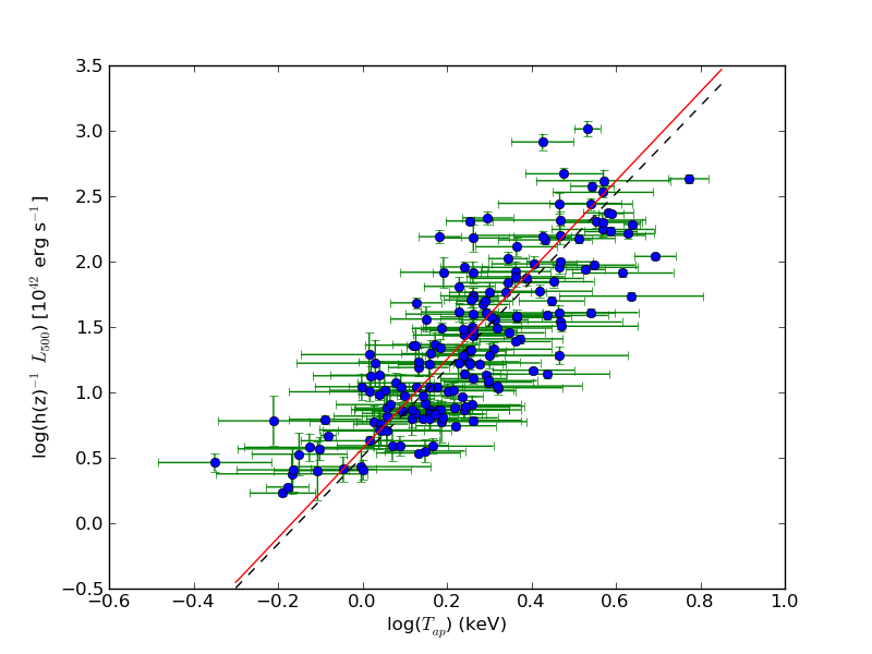
Figure 12: The relation between the X-ray bolometric luminosities $L_{500}$ and aperture temperatures $T_{ap}$ of the first cluster sample. The solid line indicates the best fit of the sample using orthogonal distance regression (ODR). The dashed line is the extrapolated relation for REXCESS sample (Pratt et al., 2009) using a BCES orthogonal fit.

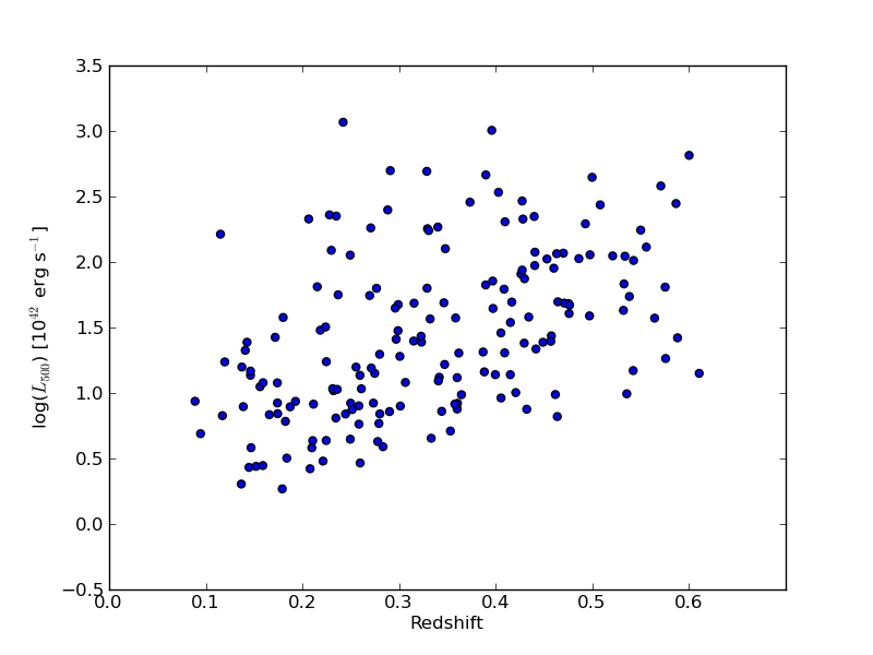
Figure 13: The distribution of the X-ray bolometric luminosities $L_{500}$ as a function of optical redshifts of the first cluster sample.

Table 2, available at the CDS, represents the first cluster sample containing as many as 175 X-ray clusters. In addition, the first cluster sample with the X-ray-optical overlay and fitted spectra for each cluster is publicly available from http://www.aip.de/groups/xray/XMM_-SDSS_-CLUSTERS. In the catalogue, we provide the cluster identification number (detection Id, detid) and its name (IAUNAME) in (cols. [1] and [2]), the right ascension and declination of X-ray emission in equinox J2000.0 (cols. [3] and [4]), the XMM-Newton observation Id (obsid) (col. [5]), the optical redshift (col. [6]), the scale at the cluster redshift in kpc/^′′ (col. [7]), the aperture and $R_{500}$ radii in kpc (col.[8] and [9]), the cluster aperture X-ray temperature $T_{ap}$ and its positive and negative errors in keV (cols. [10], [11] and [12], respectively), the aperture X-ray flux $F_{ap}$ [0.5-2] keV and its positive and negative errors in units of $10^{-14}$ erg cm^-2 s^-1 (cols. [13], [14] and [15], respectively), the aperture X-ray luminosity $L_{ap}$ [0.5-2] keV and its positive and negative errors in units of $10^{42}$ erg s^-1 (cols. [16], [17] and [18], respectively), the cluster bolometric luminosity $L_{500}$ and its error in units of $10^{42}$ erg s^-1 (cols. [19] and [20]), the cluster mass $M_{500}$ and its error in units of $10^{13}$ M$\odot$ (cols. [21] and [22]), the Galactic HI column in units $10^{22}$ cm^-2 (col.[23]), the identification number of the cluster in optical catalogue (col.[24]), the BCG right ascension and declination in equinox J2000.0 (cols. [25] and [26]) although for AMF catalogue they represent the cluster stellar mass centre, the cluster photometric redshift (col.[27]), the average spectroscopic redshift of the cluster galaxies with available spectroscopic redshifts and their number (cols.[28] and [29]), the linear offset between the cluster X-ray position and the cluster optical position (col.[30]), the optical cluster catalogue names that identify the cluster (col.[31]) (Note: the optical parameters are extracted from the first one), and the alternative name of the X-ray clusters previously identified using ROSAT, Chandra, or XMM-Newton data and its reference in NED and SIMBAD databases (col.[32] and [33]).

5 Summary and outlook

We have presented the first sample of X-ray galaxy clusters from the 2XMMi-Newton/SDSS Galaxy Cluster Survey. The survey comprises 1180 cluster candidates selected as X-ray serendipitous sources from the second XMM-Newton serendipitous source catalogue (2XMMi-DR3) that had been observed by the SDSS. A quarter of the candidates are identified as distant cluster candidates beyond z = 0.6, because there is no apparent overdensity of galaxies in the corresponding SDSS images. Another quarter of the candidates had been previously identified in optical cluster catalogues extracted from SDSS data. Our cross-correlation of the X-ray cluster candidates with four optical cluster catalogues within a matching radius of one arcmin confirmed 275 clusters and provided us with the photometric redshifts for all of them and the spectroscopic redshifts for 120 BCGs. We extracted all available spectroscopic redshifts for the cluster members from recent SDSS data. Among the confirmed cluster sample, 182 clusters have spectroscopic redshifts for at least one galaxy member. More than 80 percent of the confirmed sample are newly identified X-ray clusters and the others had been previously identified using ROSAT, Chandra, or XMM-Newton data. We reduced and analysed the X-ray data of the confirmed sample in an automated way. The X-ray temperature, flux and luminosity of the confirmed sample and their errors were derived from spectral fitting. The analysed sample in the present work contains 175 X-ray galaxy clusters with acceptable measurements of X-ray parameters (ie. with fractional errors smaller than 0.5) from reasonable quality fitting (139 objects being newly discovered in X-rays). In addition, we derived the physical properties ($R_{500}$, $L_{500}$ and $M_{500}$) of the study sample from an iterative procedure using the published scaling relations. The relation between the X-ray bolometric luminosity $L_{500}$ and aperture temperature of the sample is investigated. The slope of the relation agrees with the slope of the same relation in the REXCESS sample (Pratt et al., 2009). The present relation is derived from a large sample with low luminosities and temperatures across a wide redshift range 0.09 - 0.61.

As one extension to this project, we intend to obtain SDSS photometric redshifts of all 2XMMi-DR3 X-ray cluster candidates that have been detected in SDSS imaging. This will significantly increase the sample size and the identified fraction of the 2XMMi cluster sample. Further improvements in the accuracy of the X-ray parameters for about 10 percent of the confirmed sample will be made by analysing repeated observations of those clusters.

Table 2: The first 25 entries of the first cluster sample

detid	Name	ra	dec	obsid	z	scale	$R_{ap}$	$R_{500}$	$T_{ap}$	$+eT_{ap}$	$-eT_{ap}$	$F_{ap}$	$+eF_{ap}$	$-eF_{ap}$	$L_{ap}$	$+eL_{ap}$	$-L_{ap}$
	IAUNAME	(deg)	(deg)			kpc/′′	(kpc)	(kpc)	(keV)	(keV)	(keV)
(1)	(2)	(3)	(4)	(5)	(6)	(7)	(8)	(9)	(10)	(11)	(12)	(13)	(14)	(15)	(16)	(17)	(18)
005825	2XMM J003917.9+004200	9.82489	0.70013	0203690101	0.2801	4.24	89.14	474.51	1.07	0.33	0.42	0.51	0.17	0.22	1.27	0.46	0.40
005901	2XMM J003942.2+004533	9.92584	0.75919	0203690101	0.4152	5.50	247.28	566.70	1.83	0.42	0.18	2.19	0.23	0.19	12.70	1.32	1.07
006920	2XMM J004231.2+005114	10.63008	0.85401	0090070201	0.1468	2.57	107.87	464.68	1.41	0.28	0.33	1.09	0.41	0.30	0.62	0.19	0.17
007340	2XMM J004252.6+004259	10.71952	0.71650	0090070201	0.2595	4.02	385.77	535.23	1.98	0.64	0.32	3.29	0.40	0.27	6.39	0.71	0.55
007362	2XMM J004253.7-093423	10.72397	-9.57311	0065140201	0.4054	5.42	259.99	553.50	1.49	0.52	0.18	2.25	0.58	0.24	12.64	2.86	2.43
007881	2XMM J004334.0+010106	10.89197	1.01844	0090070201	0.1741	2.95	203.84	549.63	1.34	0.15	0.13	4.97	0.27	0.46	4.15	0.44	0.34
008026	2XMM J004350.7+004733	10.96148	0.79263	0090070201	0.4754	5.94	445.43	576.17	2.32	0.64	0.47	2.93	0.23	0.24	22.38	1.37	1.94
008084	2XMM J004401.3+000647	11.00567	0.11323	0303562201	0.2185	3.53	307.39	622.06	1.83	0.40	0.20	8.71	1.28	0.83	11.73	1.69	1.58
021508	2XMM J015917.2+003011	29.82169	0.50328	0101640201	0.2882	4.33	259.91	838.95	1.98	0.30	0.24	32.62	2.76	2.07	79.81	6.20	6.81
021850	2XMM J020342.0-074652	30.92533	-7.78128	0411980201	0.4398	5.68	341.05	752.50	3.71	1.24	0.85	10.50	0.75	0.82	62.67	5.59	6.38
030611	2XMM J023150.5-072836	37.96059	-7.47683	0200730401	0.1791	3.02	208.60	406.59	0.65	0.16	0.08	0.95	0.06	0.09	0.88	0.06	0.07
030746	2XMM J023346.9-085054	38.44543	-8.84844	0150470601	0.2799	4.24	254.58	561.31	1.78	0.55	0.45	3.26	0.74	0.55	7.49	1.57	1.13
034903	2XMM J030637.1-001803	46.65469	-0.30096	0201120101	0.4576	5.81	331.40	531.81	2.05	0.83	0.45	1.73	0.24	0.18	11.24	1.49	1.25
042730	2XMM J033757.5+002900	54.48959	0.48351	0036540101	0.3232	4.69	253.05	566.44	1.80	0.34	0.37	3.00	0.40	0.33	9.22	0.93	1.00
080229	2XMM J073605.9+433906	114.02470	43.65179	0083000101	0.4282	5.60	386.12	752.33	3.87	0.65	0.46	11.22	0.65	0.47	58.15	3.49	2.67
083366	2XMM J075121.7+181600	117.84073	18.26679	0111100301	0.3882	5.28	316.50	501.14	1.20	0.30	0.20	1.65	0.28	0.25	8.44	1.27	1.55
083482	2XMM J075427.4+220949	118.61452	22.16371	0110070401	0.3969	5.35	304.78	643.87	2.18	0.55	0.43	5.70	0.70	0.58	26.81	4.35	3.06
089735	2XMM J082746.9+263508	126.94574	26.58556	0103260601	0.3869	5.26	236.90	530.40	1.69	1.05	0.46	1.63	0.55	0.33	7.93	2.19	2.51
089885	2XMM J083146.1+525056	127.94516	52.84719	0092800201	0.5383	6.34	513.76	565.42	3.47	1.08	0.72	2.26	0.09	0.09	20.16	1.23	0.56
090256	2XMM J083454.8+553422	128.72859	55.57287	0143653901	0.2421	3.82	286.38	1102.80	3.40	0.25	0.24	165.21	3.59	4.71	258.02	5.58	6.62
090966	2XMM J083724.7+553249	129.35324	55.54712	0143653901	0.2767	4.21	315.60	677.20	1.83	0.43	0.24	11.90	1.67	1.61	26.22	4.04	2.91
092117	2XMM J084701.9+345114	131.75794	34.85384	0107860501	0.4643	5.86	369.31	582.95	2.73	1.20	0.63	2.72	0.16	0.17	18.71	1.01	1.04
092718	2XMM J084847.8+445611	132.19968	44.93637	0085150101	0.5753	6.55	353.92	567.36	1.92	0.38	0.17	2.53	0.20	0.14	30.39	3.25	1.00
097911	2XMM J092545.5+305858	141.43996	30.98303	0200730101	0.5865	6.61	357.18	713.02	3.57	0.75	0.70	7.55	0.51	0.48	86.75	6.62	7.56
098728	2XMM J093205.0+473320	143.02097	47.55565	0203050701	0.2248	3.61	259.96	567.30	1.36	0.22	0.23	5.05	0.77	0.80	7.46	1.32	1.05

Table 2: The first 25 entries of the first cluster sample, continued.

detid	$L_{500}$	$\pm eL_{500}$	$M_{500}$	$\pm eM_{500}$	nH	objid	RA	DEC	$z_{p}$	$z_{s}$	$N_{z_{s}}$	offset	opt-cats	known X-ray	ref.
												(kpc)		CLG
(1)	(19)	(20)	(21)	(22)	(23)	(24)	(25)	(26)	(27)	(28)	(29)	(30)	(31)	(32)	(33)
005825	6.93	1.96	4.05	1.03	0.0198	J003916.6+004215	9.82500	0.69981	0.2942	0.2801	1	5.10	WHL,maxBCG	-	-
005901	34.56	3.06	8.04	1.62	0.0195	587731187282018514	9.92728	0.76163	0.3873	0.4152	4	56.11	GMBCG,WHL,AMF	-	-
006920	3.82	0.76	3.29	0.79	0.0179	588015510347776148	10.63096	0.85021	0.1532	0.1468	6	36.04	GMBCG,maxBCG	-	-
007340	13.64	1.53	5.68	1.20	0.0178	J004252.7+004306	10.71964	0.71845	0.2676	0.2595	5	28.19	WHL	[PBG2005] 03	1
007362	28.75	6.27	7.40	1.66	0.0270	587727226768523625	10.72131	-9.57365	0.4054	0.0000	0	52.21	GMBCG,WHL	-	-
007881	11.95	0.89	5.61	1.17	0.0182	588015510347907142	10.89606	1.01972	0.1661	0.1741	7	45.59	GMBCG,WHL,AMF	[PBG2005] 1	1
008026	48.17	4.51	9.06	1.82	0.0179	587731187282477303	10.95832	0.78838	0.4929	0.4754	1	113.06	GMBCG,WHL	-	-
008084	30.15	4.29	8.52	1.77	0.0168	588015509274165366	11.00568	0.11512	0.2580	0.2185	3	24.13	GMBCG,WHL	-	-
021508	249.85	29.20	22.56	4.45	0.0234	588015509819293880	29.82170	0.50343	0.2882	0.0000	0	2.25	GMBCG	[VMF98] 021	2
021850	222.60	29.56	19.37	3.86	0.0187	587727884967346553	30.92570	-7.78196	0.4834	0.4398	1	16.02	GMBCG,AMF	-	-
030611	1.85	0.11	2.28	0.53	0.0318	J023149.7-072834	37.95694	-7.47613	0.2039	0.1791	2	40.11	WHL	-	-
030746	19.75	3.68	6.70	1.47	0.0300	587724240688316594	38.44672	-8.84924	0.2799	0.0000	0	23.01	GMBCG,WHL,maxBCG,AMF	-	-
034903	27.30	3.53	6.98	1.46	0.0627	588015508752892483	46.65299	-0.30216	0.4120	0.4576	1	43.63	GMBCG	-	-
042730	24.46	2.52	7.22	1.48	0.0614	588015509830107502	54.48798	0.48583	0.3220	0.3232	5	47.71	GMBCG,WHL	[PBG2005] 13	1
080229	212.68	16.29	19.09	3.67	0.0549	J073605.8+433908	114.02408	43.65224	0.4011	0.4282	2	12.85	WHL	-	-
083366	14.50	2.56	5.39	1.20	0.0520	8718.0.0.8718	117.83460	18.26690	0.3969	0.3882	1	110.47	AMF	-	-
083482	71.54	10.89	11.54	2.37	0.0617	J075427.2+220941	118.61320	22.16150	0.3937	0.3969	1	48.61	WHL	-	-
089735	20.56	6.14	6.38	1.58	0.0356	588016841246441787	126.94684	26.58608	0.4225	0.3869	2	21.17	GMBCG,WHL,AMF	-	-
089885	54.55	3.55	9.23	1.82	0.0411	J083146.4+525057	127.94344	52.84933	0.5383	0.0000	0	54.34	WHL	-	-
090256	1167.06	156.57	48.71	10.09	0.0429	587737808499048612	128.72875	55.57253	0.2033	0.2421	2	4.84	GMBCG	4C +55.16	3
090966	62.97	8.97	11.72	2.39	0.0405	8222	129.35330	55.54786	0.2780	0.2767	2	11.21	maxBCG	-	-
092117	49.68	3.40	9.27	1.83	0.0292	587732482731737444	131.75750	34.85367	0.4725	0.4643	1	8.47	GMBCG,WHL	-	-
092718	64.29	5.19	9.74	1.93	0.0279	23315.0.0.23315	132.20100	44.93770	0.5753	0.0000	0	38.44	AMF	[VMF98] 060	2
097911	279.44	31.21	19.60	3.85	0.0178	18874.0.0.18874	141.43440	30.98410	0.5865	0.0000	0	116.35	AMF	-	-
098728	17.34	2.73	6.51	1.40	0.0129	1896	143.01990	47.55527	0.2350	0.2248	1	10.65	maxBCG,AMF	-	-

1- Plionis et al. (2005); 2- Vikhlinin et al. (1998); 3- Cavagnolo et al. (2008); 4- Finoguenov et al. (2007); 5-Horner et al. (2008);
6-Dietrich et al. (2007); 7- Burenin et al. (2007); 8- Romer et al. (2000); 9- Basilakos et al. (2004); 10- Schuecker et al. (2004); 11- Sehgal et al. (2008)

Appendix A Gallery

We present a gallery of four galaxy clusters from the first cluster sample with different X-ray fluxes and data quality at different redshifts covering the whole redshift range of the sample. For each cluster, X-ray flux contours (0.2-4.5 keV) are overlaid on combined image from $r$, $i$, and $z$- SDSS images. The upper panel in each figure shows the X-ray-optical overlays. The field of view is $4^{\prime}\times 4^{\prime}$ centred on the X-ray cluster position. In each overlay, the cross-hair indicates the position of the brightest cluster galaxy (BCG), while in Figure A.4 the cross-hair indicates the cluster stellar mass centre although but it is obvious that the BCG is located at the X-ray emission peak. In each figure, the bottom panel shows the X-ray spectra (EPIC PN (black), MOS1 (green), MOS2 (red)) and the best fitting MEKAL model. The full gallery of the first cluster sample is available at http://www.aip.de/groups/xray/XMM_-SDSS_-CLUSTERS.

Figure 14: detid = 275409: 2XMMI J143929.0+024605 at $z_{s}$ = 0.1447 ($F_{ap}\ [0.5-2]\ keV=0.63\times 10^{-14}$  erg cm^-2 s^-1).

Figure 15: detid = 090256: 2XMM J083454.8+553422 at $z_{s}$ = 0.2421 ($F_{ap}\ [0.5-2]\ keV=165.21\times 10^{-14}$  erg cm^-2 s^-1).

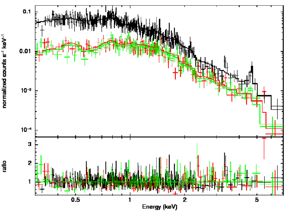
Figure 16: detid = 312615: 2XMM J091935.0+303157 at $z_{s}$ = 0.4273 ($F_{ap}\ [0.5-2]\ keV=16.03\times 10^{-14}$  erg cm^-2 s^-1).

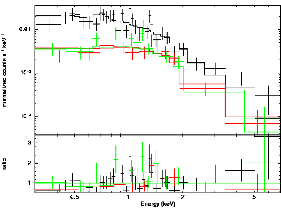
Figure 17: detid = 097911: 2XMM J092545.5+305858 at $z_{p}$ = 0.5865 ($F_{ap}\ [0.5-2]\ keV=7.59\times 10^{-14}$  erg cm^-2 s^-1).