CENTORI: a global toroidal electromagnetic two-fluid plasma turbulence code

Abstract

A new global two-fluid electromagnetic turbulence code, CENTORI, has been developed for the purpose of studying magnetically-confined fusion plasmas on energy confinement timescales. This code is used to evolve the combined system of electron and ion fluid equations and Maxwell equations in toroidal configurations with axisymmetric equilibria. Uniquely, the equilibrium is co-evolved with the turbulence, and is thus modified by it. CENTORI is applicable to tokamaks of arbitrary aspect ratio and high plasma beta. A predictor-corrector, semi-implicit finite difference scheme is used to compute the time evolution of fluid quantities and fields. Vector operations and the evaluation of flux surface averages are speeded up by choosing the Jacobian of the transformation from laboratory to plasma coordinates to be a function of the equilibrium poloidal magnetic flux. A subroutine, GRASS, is used to co-evolve the plasma equilibrium by computing the steady-state solutions of a diffusion equation with a pseudo-time derivative. The code is written in Fortran 95 and is efficiently parallelized using Message Passing Interface (MPI). Illustrative examples of output from simulations of a tearing mode in a large aspect ratio tokamak plasma and of turbulence in an elongated conventional aspect ratio tokamak plasma are provided.

PACS: 52.30.Ex, 52.35.Kt, 52.35.Ra, 52.55.Fa, 52.65.Kj

1 Introduction

Plasma confinement in tokamak experiments is determined partly by binary Coulomb collisions between charged particles, but mainly by turbulence and instabilities, which occur on scales ranging from particle Larmor radii to the system size. Understanding the nature of this turbulence is a key goal of thermonuclear fusion research, since the confinement time is one of the parameters that must be optimised in order to create burning plasma conditions. In order to simulate turbulence in tokamak plasmas it is necessary to either average the Vlasov equations of the particle species over gyro-angle (the gyrokinetic approach) or take full velocity-space moments of these equations (the fluid approach). The lower dimensionality of fluid models makes it possible to simulate larger systems over longer timescales, and for this reason fluid codes continue to play an important role in tokamak plasma modelling. Some of these codes are based on electrostatic models [1, 2] or employ flux tube geometry [3], while others are designed specifically for the purpose of simulating edge plasma phenomena, such as edge localised modes (ELMs) [4, 5]. A global magnetohydrodynamic (MHD) code NIMROD [6] has also been applied to the modelling of ELMs [7], in addition to a range of other MHD instabilities in several different toroidal configurations [8]. In order to model turbulent transport on confinement and resistive diffusion timescales in an electromagnetic global code, it is necessary to include two-fluid effects, and it is also desirable to co-evolve the equilibrium.

In this paper we describe CENTORI (Culham Emulator of Numerical TORI), a new toroidal two-fluid, electromagnetic turbulence simulation code that meets these requirements. It can be used to describe the co-evolution of turbulence, MHD instabilities and equilibrium in tokamak plasmas with arbitrary aspect ratio and high plasma beta (ratio of plasma pressure to magnetic field energy density). It is designed for the specific purpose of simulating global two-fluid electromagnetic tokamak plasma turbulence on confinement timescales, in realistic geometries and in conditions such as those found in the present-day machines MAST [9] and JET [10], and in the forthcoming international fusion experiment ITER [11]. Turbulent modes in tokamak plasmas are typically drift waves, which are predominantly electrostatic waves driven by temperature or density gradients. An important example is the ion temperature gradient mode, which has wavelengths perpendicular to the magnetic field of the order of the ion Larmor radius $\rho_{i}$ [12]. Many tokamak turbulence codes, such as the electrostatic fluid codes mentioned above and also gyro-kinetic codes such as Kinezero [13], are designed specifically for the modelling of drift waves in a fixed, prescribed plasma equilibrium. CENTORI, on the other hand, is designed to study the interaction between drift waves and MHD instabilities, which generally occur at longer wavelengths, ranging up to the system size, in a co-evolving equilibrium. However fluid codes such as CENTORI cannot be used to model explicitly instabilities that occur on the smallest tokamak-relevant spatial scales, in particular length scales below the ion Larmor radius. Phenomena on the scale of the electron skin depth $\delta_{e}$ are specifically excluded from the model used in CENTORI, since electron inertia is neglected (in any event $\delta_{e}<\rho_{i}$ unless the plasma beta is less than the electron to ion mass ratio, which is not normally the case in the core region of tokamak plasmas). The drift waves described by gyro-kinetic theory have frequencies of the order of $\rho^{*}\Omega$ where $\rho^{*}$ is particle Larmor radius normalised to the equilibrium gradient scale length and $\Omega$ is the corresponding cyclotron frequency [14]. Two-fluid theory, on the other hand, can accommodate MHD modes such as global Alfvén eigenmodes [15], which, in low beta plasmas, have frequencies higher than those of ion drift waves. CENTORI can be used to study processes occurring on timescales ranging from the reciprocal Alfvén frequency to the energy confinement time.

The physics model implemented in CENTORI is very similar to that used in CUTIE, a global two-fluid electromagnetic turbulence code which was based on periodic cylinder geometry and was restricted to large aspect ratio plasmas with circular poloidal cross-section [16]. Despite these restrictions, CUTIE has been used for a number of successful applications. For example, it was recently shown to reproduce experimentally-observed transitions to a high confinement mode of plasma operation via the control of particle fuelling in the COMPASS-D tokamak [17].

This paper is organised as follows. In Section 2 we describe the relationship between laboratory coordinates and plasma coordinates, in which the fluid and Maxwell equations are evolved in CENTORI. The form in which these equations are solved is discussed in Sections 3–5, while initial and boundary conditions are discussed in Section 6. Sections 7 and 8 are concerned respectively with the distinction made in the code between mean and fluctuating quantities, and global quantities evolved by it, such as plasma beta. In Section 9 we describe GRASS, a subroutine of CENTORI which co-evolves the plasma equilibrium using a novel pseudo-transient method. Operational and technical aspects of the CENTORI package and the code structure are discussed in Section 10, while in Section 11 we present some illustrative examples of output from a simulation of a large aspect ratio tokamak plasma.

2 Coordinate system

Before describing the physical quantities and their evolution equations, it is useful to provide a full description of the coordinate systems used in CENTORI.

2.1 Laboratory coordinates

CENTORI is used to model a toroidal plasma held in place by magnetic fields produced by external coils and by the plasma itself. A natural coordinate system to use for the laboratory frame is the right-handed cylindrical system $(R,Z,\zeta)$, where $R$ is major radius (distance from the machine’s vertical axis of symmetry), $Z$ is vertical distance (parallel to the symmetry axis), and $\zeta$ is toroidal angle (azimuthal angle around the symmetry axis). We note that

$$\nabla\zeta=-\nabla\phi=\frac{1}{R}\,\mathbf{e_{\zeta}},$$ (1)

where $\phi$ is azimuthal angle in the right-handed cylindrical system $(R,\phi,Z)$ and $\mathbf{e_{\zeta}}$ is the unit vector in the $\zeta$ direction.

2.2 Plasma coordinates

The total magnetic field in the system comprises the vacuum field, produced solely by currents flowing in conductors surrounding the plasma, plus the field generated by the currents in the plasma itself. We use the total equilibrium magnetic field to define the plasma coordinate system. The equilibrium poloidal flux function $\psi(R,Z)$ defines the equilibrium poloidal magnetic field. The quantity $\psi(R,Z)$ can evolve in a CENTORI simulation, but only on a much longer timescale than the turbulence. It is the magnetic flux per unit toroidal angle passing through the horizontal circle of radius $R$ centred at $(R=0,Z)$; it is independent of $\zeta$. When plotted in the poloidal $(R,Z)$ plane the lines of constant $\psi$ in the vicinity of the plasma form nested, closed contours (flux surfaces). The minimum value of $\psi$ within these closed surfaces lies near the centre of the plasma, and defines the location of the magnetic axis, along the circle $(R_{0},Z_{0},\zeta)$.

In a real machine the edge location of the plasma is determined by either a physical limiter or the design of the magnetic geometry. Because only the gradients of $\psi$ have physical meaning we may, for convenience, adjust $\psi$ so that the known location of the edge of the plasma is defined to lie on the $\psi=0$ contour. Figure 1 shows a typical set of $\psi$ contours in the poloidal plane.

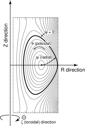
Figure 1: Typical plot of $\psi$ contours over the $(R,Z)$ grid, showing laboratory coordinates $(R,Z,\zeta$) and plasma coordinates $(\psi,\theta,\zeta)$ employed in CENTORI. This plot was obtained using the GRASS equilibrium solver (Section 9.1).

This plot is effectively the starting point for the calculations performed using CENTORI. The flux contours $\psi(R,Z)$ are determined a priori either by an external program or the equilibrium solver in the code, which is described in Section 9; they are co-evolved in time with the turbulence.

Our aim is to evolve a set of plasma quantities which are stored in arrays at a convenient set of computational grid points in a right-handed but in general non-orthogonal dimensionless plasma coordinate system $(\rho,\theta,\zeta)$. Here $\rho$ is a radial coordinate, with $\nabla\rho$ directed from the magnetic axis to the plasma edge, and $\theta$ denotes an angle in the $(R,Z)$ plane.

2.3 Radial coordinate

The radial coordinate $\rho$ is a normalised measure of $\psi$, the normalising factor being the absolute value of the poloidal flux at the magnetic axis, $\psi_{0}$. Thus, from the magnetic axis at $(R_{0},Z_{0})$ to the edge of the plasma we have $-\psi_{0}\leq\psi\leq 0$ and $0\leq\rho\leq 1$ with $\rho$ defined in terms of $\psi$ by

$$\rho\equiv 1+\psi/\psi_{0}\;.$$ (2)

The radial grid points are equally spaced in $\rho$. In the cylindrical limit $\rho$ varies approximately as $r^{2}$ where $r$ is distance from the magnetic axis. The $\rho$ contours are thus relatively far apart near the magnetic axis, as shown in Fig. 1. Because the magnetic axis is a coordinate singularity (all $\theta$ points at $\rho=0$ and a given $\zeta$ coincide), we have chosen to locate the innermost $\rho$ grid points on a contour that is slightly displaced from the axis itself.

The gradient $\nabla\rho$ in the laboratory frame is determined from the $\psi(R,Z)$ grid by fitting two-dimensional Chebyshev polynomials [18] to the known $\psi$ values at the grid points, and taking their derivatives in the $R$ and $Z$ directions. It follows from Eq. (2) that

$$\nabla\rho\equiv\frac{1}{\psi_{0}}\nabla\psi=\frac{1}{\psi_{0}}\frac{\partial\psi}{\partial R}\mathbf{e_{R}}+\frac{1}{\psi_{0}}\frac{\partial\psi}{\partial Z}\mathbf{e_{Z}},$$ (3)

where $\mathbf{e_{R}}$ and $\mathbf{e_{Z}}$ denote unit vectors in the $R$ and $Z$ directions.

2.4 Relationship between equilibrium magnetic field and plasma coordinates

The equilibrium poloidal magnetic field is given by

$$\mathbf{B}_{p}\equiv\nabla\zeta\times\nabla\psi=\psi_{0}\,(\nabla\zeta\times\nabla\rho).$$ (4)

Thus $B_{p}=\psi_{0}|\nabla\rho|/R$. The toroidal equilibrium magnetic field is given by

$$\mathbf{B}_{t}\equiv F\,\nabla\zeta,$$ (5)

where the scalar quantity $F$ is taken to be a flux function, i.e. it depends only on the radial coordinate $\rho$. This is generally a good approximation under typical tokamak conditions [19]. Thus the total equilibrium magnetic field is

$$\mathbf{B}_{\mathbf{eq}}=\psi_{0}\,(\nabla\zeta\times\nabla\rho)+F\,\nabla\zeta.$$ (6)

We define a vector potential $\mathbf{A}$ in the usual way as a vector field whose curl is equal to the magnetic field. We can write the equilibrium vector potential $\mathbf{A}_{\mathbf{eq}}$ in covariant form as follows:

$$\mathbf{A}_{\mathbf{eq}}=A_{\mbox{eq}\,\rho}\nabla\rho+A_{\mbox{eq}\,\theta}\nabla\theta+A_{\mbox{eq}\,\zeta}\nabla\zeta.$$ (7)

For convenience we choose a gauge such that the radial component of $\mathbf{A}_{\mathbf{eq}}$ vanishes, i.e.

$$A_{\mbox{eq}\,\rho}=0.$$ (8)

In terms of the remaining components of $\mathbf{A}_{\mathbf{eq}}$, the equilibrium magnetic field becomes

$$\mathbf{B}_{\mathbf{eq}}=\nabla\times\mathbf{A}_{\mathbf{eq}}=\nabla A_{\mbox{eq}\,\theta}\times\nabla\theta+\nabla A_{\mbox{eq}\,\zeta}\times\nabla\zeta.$$ (9)

Matching the poloidal components of Eqs. (6) and (9) we find that we can set

$$A_{\mbox{eq}\,\zeta}=-\psi.$$ (10)

Matching the toroidal components of Eqs. (6) and (9) we obtain

$$F\nabla\zeta=\nabla A_{\mbox{eq}\,\theta}\times\nabla\theta=\frac{\partial A_{\mbox{eq}\,\theta}}{\partial\rho}\nabla\rho\times\nabla\theta,$$ (11)

and the scalar product of this with $\nabla\zeta$ yields

$$F\nabla\zeta\cdot\nabla\zeta={F\over R^{2}}=\frac{\partial A_{\mbox{eq}\,\theta}}{\partial\rho}\nabla\zeta\cdot(\nabla\rho\times\nabla\theta)=\frac{\partial A_{\mbox{eq}\,\theta}}{\partial\rho}\mathcal{J},$$ (12)

where $\mathcal{J}\equiv\nabla\zeta\cdot(\nabla\rho\times\nabla\theta)$ is the Jacobian relating laboratory and plasma coordinates (see following subsection). The covariant poloidal component of $\mathbf{A}_{\mathbf{eq}}$ is thus given by

$$A_{\mbox{eq}\,\theta}=\int\frac{F}{\mathcal{J}R^{2}}d\rho.$$ (13)

Eqs. (8), (10) and (13) define the equilibrium vector potential $\mathbf{A}_{\mathbf{eq}}$ in covariant form; the equilibrium magnetic field $\mathbf{B}_{\mathbf{eq}}$ may be calculated by taking its curl.

The set of space variables $(\rho,\theta,\zeta)$ constitutes a quasi-orthogonal coordinate system in which $\nabla\rho\cdot\nabla\zeta=\nabla\theta\cdot\nabla\zeta=0$, but in general $\nabla\rho\cdot\nabla\theta\not=0$. Taking scalar products of $\mathbf{B}_{\mathbf{eq}}$ with the coordinate gradients we obtain

$$\mathbf{B}_{\mathbf{eq}}\cdot\nabla\rho=0,\;\;\;\;\;\mathbf{B}_{\mathbf{eq}}\cdot\nabla\theta=\psi_{0}\,(\nabla\zeta\times\nabla\rho)\cdot\nabla\theta=\psi_{0}\,\mathcal{J},\;\;\;\;\;\mathbf{B}_{\mathbf{eq}}\cdot\nabla\zeta=F/R^{2}.$$ (14)

These three equations give the contravariant components of $\mathbf{B}_{\mathbf{eq}}$ directly, thereby eliminating the need to perform a curl operation (see Section 2.6).

2.5 Poloidal coordinate

The poloidal angle $\theta$ varies from $0$ to $2\pi$ in the $(R,Z)$ plane. By convention, points at $\theta=0$ lie along the line defined by $(R\geq R_{0},Z=Z_{0})$, and $\theta$ increases in the anticlockwise direction as shown in Fig. 1. Denoting by $l$ the arc length in the poloidal plane along a given $\rho$ contour, we can write

$$\mathbf{B}_{\mathbf{eq}}\cdot\nabla\theta=B_{p}\frac{\partial\theta}{\partial l}=\psi_{0}\,\frac{|\nabla\rho|}{R}\frac{\partial\theta}{\partial l}=\psi_{0}\,\mathcal{J}.$$ (15)

To determine the distribution of $\theta$ grid points along the contour in the $(R,Z)$ plane we introduce a parameter $\tau$ and solve the following pair of Hamiltonian equations [19]:

$$\frac{dR}{d\tau}=-\frac{\partial\rho}{\partial Z}\;;\;\;\;\frac{dZ}{d\tau}=\frac{\partial\rho}{\partial R},$$ (16)

with $(R,Z)$ being stored at intermediate points as the solution proceeds. The gradients in $\rho$ are calculated using Chebyshev polynomials, as described above, and a convergence loop ensures that the contour is followed with sufficient accuracy. The arc length $l$ is given in terms of $\tau$ by

$$\frac{dl}{d\tau}=\sqrt{\left(\frac{dR}{d\tau}\right)^{2}+\left(\frac{dZ}{d\tau}\right)^{2}}=\sqrt{\left(\frac{\partial\rho}{\partial R}\right)^{2}+\left(\frac{\partial\rho}{\partial Z}\right)^{2}}=|\nabla\rho|.$$ (17)

We choose $\mathcal{J}$ to be a flux function, i.e. $\mathcal{J}=\mathcal{J}(\rho)$. This enables $\theta$ points on a given flux contour to be determined by integrating the expression

$$d\theta=R\,\mathcal{J}\,\frac{dl}{|\nabla\rho|}=R\,\mathcal{J}\,d\tau,$$ (18)

where $\mathcal{J}$ is obtained by imposing a 2$\pi$ periodicity on $\theta$:

$$\mathcal{J}(\rho)=\frac{2\pi}{\oint R\,d\tau}.$$ (19)

It is straightforward to interpolate the stored $(R,Z)$ values to determine the locations of equally-spaced $\theta$ points along the $\rho$ contour. Figure 2 shows an example of a $(\rho,\theta)$ grid.

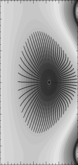
Figure 2: Typical set of $(\rho,\theta)$ grid points, superimposed on the original $\psi(R,Z)$ grid. In this case there are 129 radial grid points and 65 poloidal grid points.

The process described above can be used to map out the locations $R(\rho,\theta)$, $Z(\rho,\theta)$ along the $\rho$ contours. The partial derivatives $\partial R/\partial\rho$, $\partial R/\partial\theta$, $\partial Z/\partial\rho$ and $\partial Z/\partial\theta$ are found by fitting Chebyshev polynomials to $R$ and $Z$ along the $\rho$ direction and Fourier series in the $\theta$ direction. These provide the contravariant basis vectors of the plasma coordinate system:

$$\mathbf{b}_{\rho}\equiv\mathcal{J}^{*}\,(\nabla\theta\times\nabla\zeta)=\frac{\partial R}{\partial\rho}\,\mathbf{e_{R}}+\frac{\partial Z}{\partial\rho}\,\mathbf{e_{Z}},$$ (20)

$$\mathbf{b}_{\theta}\equiv\mathcal{J}^{*}\,(\nabla\zeta\times\nabla\rho)=\frac{\partial R}{\partial\theta}\,\mathbf{e_{R}}+\frac{\partial Z}{\partial\theta}\,\mathbf{e_{Z}},$$ (21)

$$\mathbf{b}_{\zeta}\equiv\mathcal{J}^{*}\,(\nabla\rho\times\nabla\theta)=R\,\mathbf{e_{\zeta}},$$ (22)

where $\mathcal{J}^{*}=1/\mathcal{J}$ and $\mathbf{b}_{\zeta}$ follows directly from Eq. (1); $\nabla\zeta$ is the covariant $\zeta$ basis vector and hence is reciprocal to $\mathbf{b}_{\zeta}$. We may then calculate $\mathcal{J}^{*}$ (and therefore $\mathcal{J}$) using

$$\mathcal{J}^{*}=\mathbf{b}_{\theta}\cdot(\mathbf{b}_{\zeta}\times\mathbf{b}_{\rho}),$$ (23)

and the covariant basis vectors are given by

$$\mathbf{b}^{\rho}\equiv\nabla\rho=\mathcal{J}\,(\mathbf{b}_{\theta}\times\mathbf{b}_{\zeta}),\;\;\;\;\;\mathbf{b}^{\theta}\equiv\nabla\theta=\mathcal{J}\,(\mathbf{b}_{\zeta}\times\mathbf{b}_{\rho}),\;\;\;\;\;\mathbf{b}^{\zeta}\equiv\nabla\zeta=\frac{1}{R}\mathbf{e_{\zeta}}.$$ (24)

It is straightforward to evaluate these vector products since the covariant and contravariant basis vectors are all stored with components in the laboratory frame (although they are evaluated at specified points in $(\rho,\theta)$ space, their components relative to the basis $(\mathbf{e_{R}},\mathbf{e_{Z}},\mathbf{e_{\zeta}})$ are known).

We adopt this particular algorithm to obtain the gradients and the Jacobian in order to maximise accuracy and smoothness in the results through the use of the Chebyshev/Fourier fitting method, and it also guarantees that the covariant and contravariant basis vectors are reciprocal.

2.6 Vector operations in plasma coordinate system

This section provides expressions for scalar and vector products together with differential operators in the plasma coordinate system. In what follows $\mathbf{A}$ and $\mathbf{B}$ are arbitrary vector functions, while $f$ is an arbitrary scalar function. The vector $\mathbf{A}$ has covariant representation

$$\mathbf{A}=A_{\rho}\,\mathbf{b^{\rho}}+A_{\theta}\,\mathbf{b^{\theta}}+A_{\zeta}\,\mathbf{b^{\zeta}},$$ (25)

where $A_{i}={\bf A}\cdot{\bf b}_{i}$. The corresponding contravariant representation is

$$\mathbf{A}=A^{\rho}\,\mathbf{b_{\rho}}+A^{\theta}\,\mathbf{b_{\theta}}+A^{\zeta}\,\mathbf{b_{\zeta}},$$ (26)

where $A^{i}={\bf A}\cdot{\bf b}^{i}$. The scalar product of $\mathbf{A}$ and $\mathbf{B}$ is then $\mathbf{A}\cdot\mathbf{B}=A_{i}B^{i}=A^{i}B_{i}$, where a repeated index implies summation, while the vector product is given by

$$\mathbf{A}\times\mathbf{B} = \;\,\mathcal{J}\left\{\rule{0.0pt}{11.38109pt}(A_{\theta}B_{\zeta}-A_{\zeta}B_{\theta})\mathbf{b_{\rho}}+(A_{\zeta}B_{\rho}-A_{\rho}B_{\zeta})\mathbf{b_{\theta}}+(A_{\rho}B_{\theta}-A_{\theta}B_{\rho})\mathbf{b_{\zeta}}\right\}$$ (27)

$$= \mathcal{J}^{*}\left\{\rule{0.0pt}{11.38109pt}(A^{\theta}B^{\zeta}-A^{\zeta}B^{\theta})\mathbf{b^{\rho}}+(A^{\zeta}B^{\rho}-A^{\rho}B^{\zeta})\mathbf{b^{\theta}}+(A^{\rho}B^{\theta}-A^{\theta}B^{\rho})\mathbf{b^{\zeta}}\right\}.$$

The gradient operator, which is defined in the usual way, produces a covariant vector. The divergence of $\mathbf{A}$ is evaluated using its contravariant components:

$$\nabla\cdot\mathbf{A}=\mathcal{J}\,\left\{\frac{\partial}{\partial\rho}\left(\frac{A^{\rho}}{\mathcal{J}}\right)+\frac{\partial}{\partial\theta}\left(\frac{A^{\theta}}{\mathcal{J}}\right)+\frac{\partial}{\partial\zeta}\left(\frac{A^{\zeta}}{\mathcal{J}}\right)\right\},$$ (28)

while the curl is obtained using its covariant components, and the result is a contravariant vector:

$$\nabla\times\mathbf{A}=\mathcal{J}\,\left\{\left(\frac{\partial A_{\zeta}}{\partial\theta}-\frac{\partial A_{\theta}}{\partial\zeta}\right)\mathbf{b_{\rho}}+\left(\frac{\partial A_{\rho}}{\partial\zeta}-\frac{\partial A_{\zeta}}{\partial\rho}\right)\mathbf{b_{\theta}}+\left(\frac{\partial A_{\theta}}{\partial\rho}-\frac{\partial A_{\rho}}{\partial\theta}\right)\mathbf{b_{\zeta}}\right\}.$$ (29)

The choice of $\mathcal{J}$ as a flux function considerably simplifies and speeds up many calculations.

2.7 Physical coordinates

It is convenient to perform the vector operations discussed above using the covariant and contravariant representations. However, these do not have directions, dimensions or units that are intuitive as far as the physics is concerned. We therefore define a third set of components for the vector quantities in CENTORI, which we refer to as their physical representation: “normal”, denoting the direction normal to the flux surface; “tangential”, parallel to the flux surface in the $(R,Z)$ plane; and “toroidal”, around the machine axis. The physical components are orthogonal:

$$A_{\mathbf{normal}}=\mathbf{A}\cdot\frac{\nabla\rho}{|\nabla\rho|}=\frac{A^{\rho}}{|\nabla\rho|},$$ (30)

$$A_{\mathbf{tangential}}=\mathbf{A}\cdot\frac{(\nabla\zeta\times\nabla\rho)}{|\nabla\zeta\times\nabla\rho|}=\mathbf{A}\cdot\frac{(\nabla\zeta\times\nabla\rho)}{|\nabla\rho|/R}=A_{\theta}\,\frac{\mathcal{J}\,R}{|\nabla\rho|},$$ (31)

$$A_{\mathbf{toroidal}}=\mathbf{A}\cdot\frac{\nabla\zeta}{|\nabla\zeta|}=\frac{A^{\zeta}}{|\nabla\zeta|}.$$ (32)

2.8 Flux surface-averaged quantities

It is necessary to compute flux surface-averaged quantities in CENTORI since these affect the evolving equilibrium. The flux surface average of a scalar quantity $f(\rho,\theta,\zeta)$ is given by

$$\langle f\rangle_{\rho}=\frac{\int\!\!\!\int f\,d\theta\,d\zeta/\mathcal{J}}{\int\!\!\!\int\,d\theta\,d\zeta/\mathcal{J}}={1\over 4\pi^{2}}\int\!\!\!\int f\,d\theta\,d\zeta,$$ (33)

where $f$ is evaluated at fixed $\rho$ and we have used the fact that $\mathcal{J}$ is defined to be a flux function.

3 Physics quantities

The primary quantities evolved by CENTORI are as follows: $\mathbf{v_{i}}$, ion velocity; $\mathbf{A}$, vector potential; $n_{i}$, ion number density ($=n_{e}$, electron number density, via quasi-neutrality); $T_{i}$, ion temperature; and $T_{e}$, electron temperature. In addition, a number of auxiliary quantities can be advanced in time once the primary quantities have been updated. These are: $\mathbf{v_{e}}$, electron velocity; $\Phi$, electric potential; $\mathbf{B}$, magnetic field; $\mathbf{J}$, current density; $\mathbf{E}$, electric field; $p_{i}=n_{e}\,T_{i}$, ion pressure; and $p_{e}=n_{e}\,T_{e}$, electron pressure.

These variables are normalised as follows:

$$\mathbf{v_{i}^{*}}=\frac{\mathbf{v_{i}}}{v_{A}},\mbox{\hskip 22.76228pt}\mathbf{v_{e}^{*}}=\frac{\mathbf{v_{e}}}{v_{A}},\mbox{\hskip 22.76228pt}\mathbf{A^{*}}=\frac{\mathbf{A}}{B_{0}},\mbox{\hskip 22.76228pt}\mathbf{B^{*}}=\frac{\mathbf{B}}{B_{0}},\mbox{\hskip 22.76228pt}$$ (34)

$$n_{e}^{*}=\frac{n_{e}}{\overline{n_{e}}},\mbox{\hskip 22.76228pt}T_{i}^{*}=\frac{T_{i}}{T_{i0}},\mbox{\hskip 22.76228pt}T_{e}^{*}=\frac{T_{e}}{T_{e0}},\mbox{\hskip 22.76228pt}p_{i}^{*}=n_{e}^{*}\,T_{i}^{*}=\frac{p_{i}}{p_{i0}},\mbox{\hskip 22.76228pt}p_{e}^{*}=n_{e}^{*}\,T_{e}^{*}=\frac{p_{e}}{p_{e0}},$$ (35)

where $v_{A}=B_{0}/\sqrt{4\pi\rho_{m}}\simeq B_{0}/\sqrt{4\pi\,m_{i}\,\overline{n_{e}}}$ is a typical Alfvén speed, $\rho_{m}=m_{i}\,n_{e}$ is the ion mass density, $B_{0}$ is the vacuum toroidal field at the magnetic axis, $\overline{n_{e}}$ is the volume-averaged electron number density, $T_{i0}$ is the initial ion temperature at the magnetic axis, $T_{e0}$ is the initial electron temperature at the magnetic axis, $p_{i0}=\overline{n_{e}}\,T_{i0}$ is a nominal ion pressure, $p_{e0}=\overline{n_{e}}\,T_{e0}$ is a nominal electron pressure, and $m_{i}$ is the ion mass. The quantities $B_{0}$, $T_{i0}$ and $T_{e0}$ are given nominal values by the user; $\overline{n_{e}}$ is calculated as the plasma evolution progresses, so $v_{A}$, $p_{i0}$ and $p_{e0}$ vary with time. It should be noted that the actual density and temperature values on axis are not constrained to be their initial arbitrary values, but vary as the profiles evolve. The normalised quantities listed above are all dimensionless except for $\mathbf{A^{*}}$ which has the dimensions of length.

4 Two-fluid equations

4.1 Momentum equations

The ion momentum balance equation can be written in the form

$$\rho_{m}\left(\frac{\partial\mathbf{v_{i}}}{\partial t}+\mathbf{W}\times\mathbf{v_{i}}\right)=-\nabla p_{i}-\frac{\rho_{m}}{2}\nabla\mathbf{v_{i}}^{2}+en_{e}{\bf E}+\frac{en_{e}}{c}(\mathbf{v_{i}}\times\mathbf{B})-en_{e}\eta\mathbf{J}-\rho_{m}\,\chi_{v}(\nabla\times\mathbf{W})+\mathbf{S_{v}}.$$ (36)

where $\mathbf{W}=\nabla\times\mathbf{v_{i}}$ is vorticity, $\eta$ is resistivity (assumed to be a scalar function of space and time), $\chi_{v}$ is velocity diffusivity (see Section 5.1.2), $\mathbf{S_{v}}$ is external force density (see Section 5.1.2), $e$ is proton charge and $c$ is the speed of light (we use Gaussian cgs units throughout this paper, although output from the code is in SI units, to facilitate comparison with experimental results). In the electron momentum balance equation we neglect inertial terms, momentum sources and viscosity:

$${\bf 0}=-\nabla p_{e}-en_{e}{\bf E}-{en_{e}\over c}({\bf v_{e}}\times{\bf B})+en_{e}\eta{\bf J}.$$ (37)

This is equivalent to Ohm’s law in the limit of vanishing electron mass.

4.2 Energy equations

The transfer of energy is described by the two equations

$$\frac{3}{2}n_{e}\left(\frac{\partial}{\partial t}+\mathbf{v_{i}}\cdot\nabla\right)T_{i}+p_{i}\nabla\cdot\mathbf{v_{i}}=-\nabla\cdot\mathbf{q}_{i}+S_{i},$$ (38)

$$\frac{3}{2}n_{e}\left(\frac{\partial}{\partial t}+\mathbf{v_{e}}\cdot\nabla\right)T_{e}+p_{e}\nabla\cdot\mathbf{v_{e}}=-\nabla\cdot\mathbf{q}_{e}+S_{e},$$ (39)

where $\mathbf{q}_{i,e}$ are the ion and electron heat fluxes (see Section 5.4) and $S_{i,e}$ are additional ion and electron heating sources.

4.3 Mass continuity equation

The mass continuity equation used in CENTORI is

$$\frac{\partial\rho_{m}}{\partial t}+\nabla\cdot(\rho_{m}\mathbf{v_{i}})=S_{n}-m_{i}\,\overline{n_{e}}\,v_{A}\,\nabla\cdot\Gamma_{W}^{*}+\delta_{n}-\nu_{i\parallel}(\rho_{m}-\langle\rho_{m}\rangle),$$ (40)

where $S_{n}$ is the particle source rate (see Section 5.5.1), $\nabla\cdot\Gamma_{W}^{*}$ is a term representing the effect of the Ware pinch [20] (see Section 5.4), $\delta_{n}$ is a diffusion term given by

$$\delta_{n}=\frac{2}{3}R_{0}\,\mathcal{J}\left\{\left((\chi_{ne}+\chi_{RR})\frac{\partial^{2}\rho_{m}}{\partial\rho^{2}}\right)+\frac{\langle B_{p}\rangle^{2}}{B_{p}^{2}}\left(\chi_{ne}\frac{\partial^{2}\rho_{m}}{\partial\theta^{2}}\right)\right\},$$ (41)

with $\chi_{ne}$ and $\chi_{RR}$ respectively the particle and Rechester-Rosenbluth diffusivities (see Sections 5.1 and 5.5.2). Finally in Eq. (40), $\nu_{i\parallel}$ is the parallel ion thermal relaxation rate (see Section 5.4). It is not necessary to solve an electron continuity equation since the plasma is assumed to be quasi-neutral and the current is assumed to be divergence-free.

4.4 Maxwell’s equations

The vanishing of the divergence of B is guaranteed in CENTORI through the use of the potential representation $\mathbf{B}=\nabla\times\mathbf{A}$ and the induction equation is solved for A rather than B:

$$\frac{1}{c}\frac{\partial\mathbf{A}}{\partial t}=-\mathbf{E}-\nabla\Phi.$$ (42)

Current densities ${\bf J}$ are computed using the pre-Maxwell form of Ampère’s law:

$$\mathbf{J}=\frac{c}{4\pi}\nabla\times\mathbf{B}.$$ (43)

5 Normalised physics equations and their solution

CENTORI is used to evolve the normalised quantities defined by Eqs.  (34) and (35) rather than the absolute values of velocity, magnetic field, and so on. In this section we explain how the physics equations themselves are normalised. Unless otherwise stated, all of the normalised equations have the dimensions of reciprocal length. The equations are solved by using finite differences to approximate all of the derivatives; the solution method is thus entirely non-spectral. A key advantage of this approach is that parallelisation of the code is then relatively straightforward, and yields good scalability results (see Section 10). On the other hand the finite-element method, used, for example, in NIMROD [6], is particularly well-suited to modelling the edge regions of plasmas with strongly-shaped poloidal cross-sections.

5.1 Normalised ion momentum equation

All three physical components of $\mathbf{v_{i}^{*}}$ are evolved, with subscript “1” labelling the normal direction, subscript “2” the tangential direction, and subscript “3” the toroidal direction. We define a normalised vorticity $\mathbf{W^{*}}$:

$$\mathbf{W^{*}}\equiv\frac{\mathbf{W}}{v_{A}}=(\nabla\times\mathbf{v_{i}^{*}}).$$ (44)

It should be noted that $\mathbf{W^{*}}$ has the dimensions of reciprocal length. Using also the normalizations introduced previously, dividing by $v_{A}^{2}m_{i}\overline{n_{e}}n_{e}^{*}$, defining the following quantities

$$\beta_{i0}\equiv\frac{4\pi\,p_{i0}}{B_{0}^{2}}=\frac{p_{i0}}{v_{A}^{2}\,m_{i}\,\overline{n_{e}}},\;\;\;\;\;\;\beta_{e0}\equiv\frac{4\pi\,p_{e0}}{B_{0}^{2}}=\frac{T_{e0}}{v_{A}^{2}\,m_{i}},\;\;\;\;\;\;D_{v}\equiv\frac{\chi_{v}}{v_{A}},\;\;\;\;\;\;\mathbf{S_{v}^{*}}\equiv\frac{\mathbf{S_{v}}}{v_{A}^{2}\,m_{i}\,\overline{n_{e}}}=\frac{4\pi\,\mathbf{S_{v}}}{B_{0}^{2}},$$

and introducing an additional term related to the Rechester-Rosenbluth diffusivity $D_{RR}$ [21] [see Eq. (71)], we find that the ion momentum equation can be written in the form

$$\frac{1}{v_{A}}\frac{\partial\mathbf{v_{i}^{*}}}{\partial t} = -\left[\mathbf{W^{*}}+\frac{\omega_{ci}}{v_{A}}\mathbf{B^{*}}\right]\times\mathbf{v_{i}^{*}}-\beta_{i0}\frac{\nabla p_{i}^{*}}{n_{e}^{*}}-\beta_{e0}\nabla\Phi^{*}-\frac{1}{2}\nabla\mathbf{v_{i}^{*}}^{2}+\frac{\mathbf{S_{v}^{*}}}{n_{e}^{*}}$$ (45)

$$+\frac{\omega_{ci}}{v_{A}}\mathbf{B}_{\mathbf{eq}}^{*}\times\left(D_{RR}\frac{\nabla\langle n_{e}^{*}\rangle}{\langle n_{e}^{*}\rangle}\right)-D_{v}\,(\nabla\times\mathbf{W^{*}})-{\omega_{ci}\over v_{A}}\left[{1\over v_{A}}\frac{\partial\mathbf{A^{*}}}{\partial t}+\eta^{*}\mathbf{J^{*}}\right],$$

where $\mathbf{J^{*}}\equiv 4\pi\mathbf{J}/(cB_{0})$, $\eta^{*}\equiv c^{2}\eta/(4\pi v_{A})$, and $\omega_{ci}=eB_{0}/(m_{i}c)$. To reduce problems arising from short wavelength modes in the radial direction, the momentum equation is supplemented by artificial damping terms:

$$\frac{1}{v_{A}}\frac{\partial}{\partial t}\left(v_{i,\,\mbox{normal}}^{*}\right)=\ldots-\delta_{v}\,v_{i,\,\mbox{normal}}^{*},$$ (46)

where $\delta_{v}=0.5\nu_{i\parallel}/v_{A}$, $\nu_{i\parallel}$ being the parallel ion thermal relaxation rate [Eq. (75)]. A similar damping term is applied in the tangential direction. The dimensionless damping rate used in the code is $\delta_{v}^{*}=v_{A}\Delta t\delta_{v}$.

5.1.1 Evolution of normalised momentum equation

In the current version of CENTORI we neglect the $(1/v_{A})\partial{\bf A}^{*}/\partial t$ and ${\bf J}^{*}$ terms on the right hand side of Eq. (45). In tokamak plasmas there is generally a large separation between drift and Alfvén timescales, with the consequence that turbulent fluctuations are predominantly electrostatic in nature, and the inductive part of the electric field term plays only a minor role in the ion momentum equation. In Section 11.2 we will illustrate this point using results from a CENTORI simulation. The ${\bf J}^{*}$ term in Eq. (45) is small by virtue of the fact that tokamak plasmas tend to have very high Lundquist numbers, i.e. are close to being perfectly conducting.

In Eq. (45) it is not straightforward to convert $\delta\equiv-D_{v}(\nabla\times\mathbf{W^{*}})$ into finite differences, due to the non-orthogonal nature of the coordinate system. We approximate it by the expression

$$\delta\simeq R_{0}\,\mathcal{J}\,D_{v}\left(\frac{\partial^{2}\mathbf{v_{i}^{*}}}{\partial\rho^{2}}+\frac{\langle B_{p}\rangle^{2}}{B_{p}^{2}}\frac{\partial^{2}\mathbf{v_{i}^{*}}}{\partial\theta^{2}}\right).$$ (47)

We are assuming here that the contribution of viscosity to the ion momentum equation can be well-approximated by a term proportional to $\nabla^{2}{\bf v}_{i}^{*}$. We are thus neglecting the $\nabla(\nabla\cdot{\bf v}_{i}^{*})$ term in $\nabla\times{\bf W}^{*}$ (although the flows described by CENTORI are in general compressible); it is not necessary to include this term in order to model the neoclassical and turbulent damping of flows [22]. The factor containing $B_{p}$ is present to take account of the spacing of adjacent points in the $\theta$ direction being proportional to the local poloidal field [see Eq. (15)]. Adopting the convention that subscripts $j$, $k$ and $l$ label array elements in the $\rho$, $\theta$ and $\zeta$ directions respectively, while superscripts $N$ label time, we approximate $\delta$ by the central difference expression

$$\delta = \frac{R_{0}\,\mathcal{J}_{j,k}\,D_{v\,j,k,l}}{(\Delta\rho)^{2}}\left(\mathbf{v_{i}^{*}}_{j+1,k,l}^{N+1}+\mathbf{v_{i}^{*}}_{j-1,k,l}^{N+1}-2\mathbf{v_{i}^{*}}_{j,k,l}^{N+1}\right)$$ (48)

$$+\frac{R_{0}\,\mathcal{J}_{j,k}\,D_{v\,j,k,l}}{(\Delta\theta)^{2}}\frac{\langle B_{p}\rangle^{2}}{B_{p\,j,k,l}^{2}}\left(\mathbf{v_{i}^{*}}_{j,k+1,l}^{N}+\mathbf{v_{i}^{*}}_{j,k-1,l}^{N}-2\mathbf{v_{i}^{*}}_{j,k,l}^{N+1}\right).$$

We also introduce purely numerical diffusion terms, with coefficients $\epsilon_{\rho}$, $\epsilon_{\theta}$ and $\epsilon_{\zeta}$, which are designed to remove variations in $\mathbf{v_{i}^{*}}$ of similar length scale to the separation of adjacent grid points. It is evident that the resultant finite-difference equations are consistent with the governing partial differential equations as the mesh sizes tend to infinity. These effectively suppress spurious oscillations at wave numbers corresponding to inverse mesh size. Unlike the turbulent diffusivities, they are non-zero even when the turbulent fluctuation amplitudes go to zero for any fixed mesh size. Thus the finite difference approximation to the momentum equation is of the form

$$\mathbf{v_{i}^{*}}_{j,k,l}^{N+1} = \mathbf{v_{i}^{*}}_{j,k,l}^{N}+\frac{\epsilon_{\rho}}{2}\left(\mathbf{v_{i}^{*}}_{j+1,k,l}^{N+1}+\mathbf{v_{i}^{*}}_{j-1,k,l}^{N+1}-2\mathbf{v_{i}^{*}}_{j,k,l}^{N+1}\right)$$ (49)

$$+\frac{\epsilon_{\theta}}{2}\left(\mathbf{v_{i}^{*}}_{j,k+1,l}^{L}+\mathbf{v_{i}^{*}}_{j,k-1,l}^{L}-2\mathbf{v_{i}^{*}}_{j,k,l}^{N+1}\right)+\frac{\epsilon_{\zeta}}{2}\left(\mathbf{v_{i}^{*}}_{j,k,l+1}^{L}+\mathbf{v_{i}^{*}}_{j,k,l-1}^{L}-2\mathbf{v_{i}^{*}}_{j,k,l}^{N+1}\right).+\mbox{\ldots}$$

Here, superscripts $L$ (“latest”) indicate the most up-to-date (most time-advanced) values available. This is to avoid the use of “new” values at adjacent $\theta$ and $\zeta$ points (i.e. at $k\pm 1$, $l\pm 1$); these would appear as undesirable off-diagonal terms in the tridiagonal matrix equation. Typically, $\mathbf{v_{i}^{*}}^{L}\equiv\mathbf{v_{i}^{*}}^{N+1}$ from the previous iteration. The numerical diffusion coefficients $\epsilon_{\rho}$, $\epsilon_{\theta}$ and $\epsilon_{\zeta}$ have the following forms:

$$\epsilon_{\rho}=\frac{\sqrt{\rho}}{N_{\psi}^{2}},\;\;\;\;\;\;\epsilon_{\theta}=\frac{\sqrt{\rho}}{2\pi^{2}N_{\theta}^{2}},\;\;\;\;\;\;\epsilon_{\zeta}=\frac{1}{8\pi^{2}N_{\zeta}^{2}},$$

where $N_{\psi}$, $N_{\theta}$ and $N_{\zeta}$ are the numbers of grid intervals in the respective directions.

Dropping the $k$ and $l$ subscripts on velocity components, the finite difference approximation to the momentum equation can be written in the block tridiagonal matrix equation form

$$\underline{\mathbf{A}}_{j}\mathbf{v_{i}^{*}}_{j-1}^{N+1}+\underline{\mathbf{B}}_{j}\mathbf{v_{i}^{*}}_{j}^{N+1}+\underline{\mathbf{C}}_{j}\mathbf{v_{i}^{*}}_{j+1}^{N+1}=\mathbf{R}_{j},$$ (50)

where $\underline{\mathbf{A}}_{j}$, $\underline{\mathbf{B}}_{j}$, $\underline{\mathbf{C}}_{j}$ are $3\times 3$ matrices and $\mathbf{R}_{j}$ is a vector that depends on the latest ($L$) values of velocity components as well as those of the previous timestep. Equation (50) is solved for the normalised ion velocity $\mathbf{v_{i}^{*}}$ at the new timestep using a standard predictor-corrector scheme, with $\mathbf{v_{i}^{*}}_{j}^{L}$ converging to $\mathbf{v_{i}^{*}}_{j}^{N+1}$. We then subtract the flux surface-averaged normal component of $\mathbf{v_{i}^{*}}$, so that only a fluctuating part remains.

5.1.2 Momentum sources and transport

Presently only a toroidal momentum source is included in CENTORI; the profile is given by

$$S_{v,tor}^{*}(\rho)\equiv f_{mom}\,\frac{4\pi}{B_{0}^{2}}\,\frac{P_{aux,i}(\rho)+P_{aux,e}(\rho)}{v_{th,i}(0)},$$ (51)

where $P_{aux,i/e}$ is the external heating power per unit volume provided to the ions/electrons, $v_{th,i}(0)=(2T_{i}(0)/m_{i})^{1/2}$ is the ion thermal speed at the magnetic axis and $f_{mom}$ is a user-defined multiplier which matches the total momentum provided to the plasma with experiment.

Turbulent diffusivity terms are included in the full definition of the normalised velocity diffusivity $D_{v}$ [see Eq. (45)]:

$$D_{v}(\rho,\theta,\zeta)=\frac{\chi_{v,\mbox{\scriptsize user}}}{v_{A}}\left(1+q\langle R\rangle^{2}\sqrt{\frac{m_{i}}{m_{e}}}\left[f_{JJ}\,\tilde{\mathbf{J^{*}}}^{2}+\tilde{\mathbf{W^{*}}}^{2}\right]\right)+\frac{\chi_{v,\mbox{\scriptsize classical}}}{v_{A}},$$ (52)

where $\chi_{v,\mbox{\scriptsize user}}$ is user-specified, $\tilde{\mathbf{J^{*}}}^{2}$ is a normalised measure of entropy and $\tilde{\mathbf{W^{*}}}^{2}$ is a normalised enstrophy ($\tilde{\mathbf{J^{*}}}$ and $\tilde{\mathbf{W^{*}}}$ being the fluctuating parts of the normalised current density and vorticity respectively). The parameter $f_{JJ}$ is a user-defined multiplier between 0 and 1. The final term in $D_{v}$ is a Gyro-Bohm diffusivity:

$$\chi_{v,\mbox{\scriptsize classical}}(\rho)=f_{\chi c}\,\frac{v_{th,i}\,\rho_{i}^{2}}{a},$$ (53)

with $0\leq f_{\chi c}\leq 1$ a user-defined multiplier and $\rho_{i}$ the ion gyroradius.

5.2 Evolution of normalised electron velocity

The normalised electron velocity $\mathbf{v_{e}^{*}}$ is determined directly from $\mathbf{v_{i}^{*}}$ and $\mathbf{J^{*}}$ by noting that the net current density $\mathbf{J}$ is given by

$$\mathbf{J}=e\,n_{e}\,(\mathbf{v_{i}}-\mathbf{v_{e}}).$$ (54)

Hence

$$\mathbf{v_{e}^{*}}=\mathbf{v_{i}^{*}}-\frac{c\,B_{0}}{4\pi\,e\,\overline{n_{e}}\,n_{e}^{*}\,v_{A}}\mathbf{J^{*}}.$$ (55)

5.3 Evolution of electromagnetic quantities

5.3.1 Normalised Ampère’s Law

It is evident from the definitions of $\mathbf{B^{*}}$ and $\mathbf{J^{*}}$ that Ampère’s law has the normalised form

$$\mathbf{J^{*}}=\nabla\times\mathbf{B^{*}}.$$ (56)

Note that $\mathbf{B^{*}}$ is dimensionless while $\mathbf{J^{*}}$ has the dimensions of reciprocal length.

5.3.2 Normalised Faraday law and Ohm’s law

Ohm’s law [Eq. (37)] can be written in the form

$$\mathbf{E}=-\frac{\mathbf{v_{e}}\times\mathbf{B}}{c}-\frac{\nabla p_{e}}{e\,n_{e}}+\eta\mathbf{J}.$$ (57)

We divide the electric field into ideal and resistive parts by writing

$$\mathbf{E}_{\rm ideal}=-\frac{\mathbf{v_{e}}\times\mathbf{B}}{c}-\frac{\nabla p_{e}}{e\,n_{e}},$$

$$\mathbf{E}_{\rm res}=\eta\mathbf{J},$$

and write Faraday’s law in the form

$$\frac{1}{c}\frac{\partial\mathbf{A}}{\partial t}=-\mathbf{E}_{\rm ideal}-\nabla\Phi-\mathbf{E}_{\rm res}=-\left(-\frac{\mathbf{v_{e}}\times\mathbf{B}}{c}-\frac{\nabla p_{e}}{e\,n_{e}}\right)-\nabla\Phi-\eta\mathbf{J}.$$

We can thus write

$$\frac{B_{0}}{c}\frac{\partial\mathbf{A^{*}}}{\partial t}=-\left(-\frac{v_{A}\,B_{0}}{c}\,\mathbf{v_{e}^{*}}\times\mathbf{B^{*}}-\frac{p_{e0}}{e\,\overline{n_{e}}}\,\frac{\nabla p_{e}^{*}}{n_{e}^{*}}\right)-\nabla\Phi-\frac{c\,B_{0}}{4\pi}\,\eta\mathbf{J^{*}},$$

and hence, multiplying by $c/(v_{A}\,B_{0})$, we obtain

$$\frac{1}{v_{A}}\frac{\partial\mathbf{A}}{\partial t}=\left(\mathbf{v_{e}^{*}}\times\mathbf{B^{*}}+\frac{c\,p_{e0}}{v_{A}\,B_{0}\,e\,\overline{n_{e}}}\,\frac{\nabla p_{e}^{*}}{\,n_{e}^{*}}\right)-\frac{c}{v_{A}\,B_{0}}\,\nabla\Phi-\frac{c^{2}}{4\pi\,v_{A}}\,\eta\mathbf{J^{*}}.$$

We thus obtain the normalised Faraday’s law

$$\frac{1}{v_{A}}\frac{\partial\mathbf{A^{*}}}{\partial t}=-\mathbf{E^{*}}-\frac{c\,T_{e0}}{v_{A}\,B_{0}\,e}\,\nabla\Phi^{*},$$ (58)

where the normalised electric potential $\Phi^{*}$ is defined as $e\Phi/T_{e0}$ and the normalised electric field $\mathbf{E^{*}}$ is defined by a normalised Ohm’s law

$$\mathbf{E^{*}}\equiv\frac{c}{v_{A}\,B_{0}}\mathbf{E}=\left(-\mathbf{v_{e}^{*}}\times\mathbf{B^{*}}-\frac{c\,T_{e0}}{v_{A}\,B_{0}\,e}\,\frac{\nabla p_{e}^{*}}{\,n_{e}^{*}}\right)+\eta^{*}\mathbf{J^{*}},$$ (59)

the term in parentheses being the ideal part and the remainder the resistive part.

5.3.3 Evolution of normalised Faraday’s law

The mean electrostatic potential $\langle\Phi^{*}\rangle$ is obtained from mean radial momentum balance. Taking a flux surface average of the covariant $\rho$ component of the normalised momentum equation [Eq. (45)], neglecting contributions to the pressure gradient term that are nonlinear in flux surface variations of $n_{e}^{*}$ and $T_{i}^{*}$, and using the fact that the flux surface average of the radial component of $\mathbf{v_{i}}$ must vanish on turbulent timescales to ensure ambipolarity, we obtain

$$0=-\left\langle\left\{\left[\mathbf{W^{*}}+\frac{\omega_{ci}}{v_{A}}\mathbf{B^{*}}\right]\times\mathbf{v_{i}^{*}}\right\}_{\rho}\right\rangle-\frac{\beta_{i0}}{\langle n_{e}^{*}\rangle}\frac{d\langle p_{i}^{*}\rangle}{d\rho}-\beta_{e0}\frac{d\langle\Phi^{*}\rangle}{d\rho}-\frac{1}{2}\frac{d\langle\mathbf{v_{i}^{*}}^{2}\rangle}{d\rho}.$$

Rearranging and integrating with respect to $\rho$, we obtain the mean electrostatic potential:

$$\langle\Phi^{*}\rangle=-{\beta_{i0}\over\beta_{e0}}\int_{0}^{\rho}\frac{1}{\langle n_{e}^{*}\rangle}\frac{d\langle p_{i}^{*}\rangle}{d\rho}d\rho-\frac{1}{2\beta_{e0}}\left\{\langle\mathbf{v_{i}^{*}}^{2}\rangle(\rho)-\langle\mathbf{v_{i}^{*}}^{2}\rangle(0)\right\}-{1\over\beta_{e0}}\int_{0}^{\rho}\left\langle\left\{\left[\mathbf{W^{*}}+\frac{\omega_{ci}}{v_{A}}\mathbf{B^{*}}\right]\times\mathbf{v_{i}^{*}}\right\}_{\rho}\right\rangle\,d\rho.$$

In the standard version of CENTORI we define the total electrostatic potential $\Phi^{*}$ using the adiabaticity relation

$$\Phi^{*}=\langle\Phi^{*}\rangle+\langle T_{e}^{*}\rangle\ln\left(\frac{n_{e}^{*}}{\langle n_{e}^{*}\rangle}\right),$$ (60)

which follows from electron force balance along the magnetic field in the limit of vanishing electron mass [23]. We can write

$$\frac{\partial\mathbf{A^{*}}}{\partial t}=\frac{\partial\tilde{\mathbf{A^{*}}}}{\partial t},$$ (61)

where $\tilde{\mathbf{A^{*}}}$ is the fluctuating part of $\mathbf{A^{*}}$. It follows from Eqs. (58) and (59) that

$$\frac{1}{v_{A}}\frac{\partial\tilde{\mathbf{A^{*}}}}{\partial t}=\mathbf{v_{e}^{*}}\times\mathbf{B^{*}}+\frac{c\,T_{e0}}{v_{A}\,B_{0}\,e}\left(\frac{\nabla p_{e}^{*}}{n_{e}^{*}}-\nabla\Phi^{*}\right)-\mathbf{E^{*}}_{\rm res}.$$

The scalar product of this equation with $\mathbf{B^{*}}$ yields

$$\frac{1}{v_{A}}\mathbf{B^{*}}\cdot\frac{\partial\tilde{\mathbf{A^{*}}}}{\partial t}+\mathbf{B^{*}}\cdot\mathbf{E^{*}}_{\rm res}=\frac{c\,T_{e0}}{v_{A}\,B_{0}\,e}\mathbf{B^{*}}\cdot\left(\frac{\nabla p_{e}^{*}}{n_{e}^{*}}-\nabla\Phi^{*}\right)$$ (62)

Approximating the time-dependent terms on the left hand side by replacing $\mathbf{B^{*}}$ with $\mathbf{B}_{\mathbf{eq}}^{*}$, we obtain

$$\frac{1}{v_{A}}\frac{\partial}{\partial t}\left(\mathbf{B}_{\mathbf{eq}}^{*}\cdot\tilde{\mathbf{A^{*}}}\right)=\frac{c\,T_{e0}}{v_{A}\,B_{0}\,e}\left\{\mathbf{B}_{\mathbf{eq}}^{*}\cdot\left(\frac{\nabla p_{e}^{*}}{n_{e}^{*}}-\nabla\Phi^{*}\right)+\tilde{\mathbf{B^{*}}}\cdot\left(\frac{\nabla p_{e}^{*}}{n_{e}^{*}}-\nabla\Phi^{*}\right)\right\}-\mathbf{B}_{\mathbf{eq}}^{*}\cdot\mathbf{E^{*}}_{\rm res},$$

where $\tilde{\mathbf{B^{*}}}$ is the normalised fluctuating part of the magnetic field. Neglecting magnetosonic waves (i.e. the poloidal component of $\tilde{\mathbf{A^{*}}}$), the covariant representation of $\tilde{\mathbf{A^{*}}}$ reduces to

$$\tilde{\mathbf{A^{*}}}=\tilde{A^{*}_{\zeta}}\nabla\zeta.$$

In this limit

$$\tilde{\mathbf{B^{*}}}\equiv\nabla\times\tilde{\mathbf{A^{*}}}=\nabla\times\left(\tilde{A^{*}_{\zeta}}\nabla\zeta\right)=\nabla\tilde{A^{*}_{\zeta}}\times\nabla\zeta,$$

and hence

$$\frac{1}{v_{A}}\frac{\partial}{\partial t}\left(\mathbf{B}_{\mathbf{eq}}^{*}\cdot\tilde{\mathbf{A^{*}}}\right)=\frac{c\,T_{e0}}{v_{A}\,B_{0}\,e}\left\{\mathbf{B}_{\mathbf{eq}}^{*}\cdot\left(\frac{\nabla p_{e}^{*}}{n_{e}^{*}}-\nabla\Phi^{*}\right)+\nabla\zeta\cdot\left(\left(\frac{\nabla p_{e}^{*}}{n_{e}^{*}}-\nabla\Phi^{*}\right)\times\nabla\tilde{A^{*}_{\zeta}}\right)\right\}-\mathbf{B}_{\mathbf{eq}}^{*}\cdot\mathbf{E^{*}}_{\rm res}.$$

Using the expression for $\Phi^{*}$ [Eq. (60)] and the fact that $\mathbf{B}_{\mathbf{eq}}^{*}\cdot\nabla\langle f\rangle=0$ for any $f$ since $\nabla\langle f\rangle$ is purely radial and $\mathbf{B}_{\mathbf{eq}}^{*}$ has no radial component, we obtain

$$\mathbf{B}_{\mathbf{eq}}^{*}\cdot\left(\frac{\nabla p_{e}^{*}}{n_{e}^{*}}-\nabla\Phi^{*}\right)=\frac{\mathbf{B}_{\mathbf{eq}}^{*}}{n_{e}^{*}}\cdot\nabla(n_{e}^{*}\tilde{T_{e}^{*}}),$$

and hence, using the fact that $\mathbf{B}_{\mathbf{eq}}^{*}\cdot\tilde{\mathbf{A^{*}}}=F\tilde{A^{*}_{\zeta}}/(B_{0}R^{2})$,

$$\frac{1}{v_{A}}\frac{F}{B_{0}R^{2}}\frac{\partial\tilde{A^{*}_{\zeta}}}{\partial t}=\frac{c\,T_{e0}}{v_{A}\,B_{0}\,e}\left\{\frac{\mathbf{B}_{\mathbf{eq}}^{*}}{n_{e}^{*}}\cdot\nabla(n_{e}^{*}\tilde{T_{e}^{*}})+\nabla\zeta\cdot\left[\left(\frac{\nabla p_{e}^{*}}{n_{e}^{*}}-\nabla\Phi^{*}\right)\times\nabla\tilde{A^{*}_{\zeta}}\right]\right\}-\mathbf{B}_{\mathbf{eq}}^{*}\cdot\mathbf{E^{*}}_{\rm res}.$$ (63)

We represent $-\mathbf{B}_{\mathbf{eq}}^{*}\cdot\mathbf{E^{*}}_{\rm res}$ as a diffusion term in this equation by writing

$$-\mathbf{B}_{\mathbf{eq}}^{*}\cdot\mathbf{E^{*}}_{\rm res}\simeq\frac{F}{B_{0}R^{2}}R_{0}\,\mathcal{J}\,D_{\eta}\left(\frac{\partial^{2}\tilde{A^{*}_{\zeta}}}{\partial\rho^{2}}+\frac{\langle B_{p}\rangle^{2}}{B_{p}^{2}}\frac{\partial^{2}\tilde{A^{*}_{\zeta}}}{\partial\theta^{2}}\right),$$

where the normalised resistive diffusivity is given by

$$D_{\eta}(\rho,\theta,\zeta)=\eta^{*}+\frac{\chi_{\eta}}{v_{A}}\left(1+q\langle R\rangle^{2}\sqrt{\frac{m_{i}}{m_{e}}}\left[f_{JJ}\,\tilde{\mathbf{J^{*}}}^{2}+\tilde{\mathbf{W^{*}}}^{2}\right]\right),$$

$\chi_{\eta}$ being a user-defined diffusivity. Turbulent diffusivity terms are present to damp out fluctuations occurring at the smallest length scales; these tend to be in the poloidal direction, close to the magnetic axis. Introducing a parameter $M_{A}\equiv B_{0}R^{2}/F$ we can write

$$\frac{1}{v_{A}}\frac{\partial\tilde{A^{*}_{\zeta}}}{\partial t} = \frac{c\,T_{e0}}{v_{A}\,B_{0}\,e}\,M_{A}\,\left\{\frac{\mathbf{B}_{\mathbf{eq}}^{*}}{n_{e}^{*}}.\nabla(n_{e}^{*}\tilde{T_{e}^{*}})+\nabla\zeta.\left[\left(\frac{\nabla p_{e}^{*}}{n_{e}^{*}}-\nabla\Phi^{*}\right)\times\nabla\tilde{A^{*}_{\zeta}}\right]\right\}$$

$$+R_{0}\,\mathcal{J}\,D_{\eta}\left(\frac{\partial^{2}\tilde{A^{*}_{\zeta}}}{\partial\rho^{2}}+\frac{\langle B_{p}\rangle^{2}}{B_{p}^{2}}\frac{\partial^{2}\tilde{A^{*}_{\zeta}}}{\partial\theta^{2}}\right).$$

Finally, as in the case of the momentum equation [cf. Eq. (49)], we add numerical diffusion terms to the right hand side of the normalised Faraday’s law.

The above equation is approximated by a finite difference equation which may be written in the one-dimensional tridiagonal matrix form

$$\mathcal{A}_{j}\,A^{*\,N+1}_{\zeta\,j-1}+\mathcal{B}_{j}\,A^{*\,N+1}_{\zeta\,j}+\mathcal{C}_{j}\,A^{*\,N+1}_{\zeta\,j+1}=\mathcal{R}_{j},$$ (64)

where subscripts and superscripts have the same meaning as those in the finite difference approximation to the momentum equation, the coefficients $\mathcal{A}_{j}$, $\mathcal{B}_{j}$ and $\mathcal{C}_{j}$ do not depend explicitly on $A^{*}_{\zeta}$, while $\mathcal{R}_{j}$ depends on the latest estimate of this quantity as well as its value at the old timestep and also the latest estimate and old value of $A^{*}_{\theta}$. As in the case of the velocity components, $A^{*}_{\zeta}$ at the new time is determined by solving the above tridiagonal matrix equation using a predictor-corrector scheme. To ensure that only the fluctuating part is actually evolved, the flux surface average of $A^{*}_{\zeta}$ is evaluated, and subtracted from $A^{*}_{\zeta}$ to determine $\tilde{A^{*}_{\zeta}}$ at the new time.

5.3.4 Plasma resistivity

In terms of the flux surface-averaged density, the Spitzer resistivity is given by [24]

$$\eta_{\mbox{\scriptsize Spitzer}}(\rho)=\frac{m_{e}}{2e^{2}\langle n_{e}\rangle\tau_{ce}},$$ (65)

where

$$\tau_{ce}(\rho)=\frac{3\sqrt{m_{e}}\langle T_{e}\rangle^{3/2}}{4\sqrt{2\pi}\langle n_{e}\rangle\lambda e^{4}},$$ (66)

is the electron collision time, $\lambda$ being the Coulomb logarithm. In a toroidal plasma this is modified by neoclassical effects, which, for singly-charged ions, we model using the expression

$$K_{\eta}=\frac{1+\nu_{e}^{*}}{(1-\epsilon^{1/2})^{2}+\nu_{e}^{*}},$$ (67)

where

$$\nu_{e}^{*}=\frac{\sqrt{2}qR_{0}}{\epsilon^{3/2}v_{th,e}\tau_{ce}},$$ (68)

is the dimensionless electron collisionality, $q$ being the safety factor of the flux surface in question, and $\epsilon=a\rho^{1/2}/R_{0}$ is the local inverse aspect ratio. The resistivity is thus

$$\eta(\rho)=K_{\eta}\eta_{\mbox{\scriptsize Spitzer}(\rho)}.$$ (69)

In the banana regime ($\nu_{e}^{*}\ll 1$) the above expression for $K_{\eta}$ yields a resistivity which has the appropriate limiting behaviour as $\epsilon\to 0$ and $\epsilon\to 1$ [25]; the $\nu_{e}^{*}$ dependence ensures that $K_{\eta}\to 1$ in the limit of high collisionality, as required.

5.3.5 Evolution of toroidal field parameter $F$

The loop voltage $V_{F}$ is related via the resistive MHD form of Ohm’s law to the part of the toroidal current associated with $FF^{\prime}$:

$$\frac{2V_{F}}{c\,\eta}=-FF^{\prime}.$$

Defining $V_{F}^{*}=V_{F}/2\pi$, it is straightforward to show that the above equation has the following solution for $F$:

$$F(\rho)=\pm\sqrt{F_{vac}^{2}+\frac{8\pi}{c}\psi_{0}V_{F}^{*}\int_{\rho}^{1}\frac{d\mu}{\eta(\mu)}},$$

where $F_{vac}$ is the vacuum value of $F$, i.e. $F_{vac}=F$ at and outside the plasma boundary. The plus/minus sign in this expression takes into account the possibility of a reversal in the sign of the toroidal magnetic field.

5.4 Normalised Energy Equations

We consider here the electron energy equation; the ion equation is treated in a similar manner. From Eq. (39) we have

$$\frac{3}{2}\frac{\partial T_{e}}{\partial t}+\frac{3}{2}\mathbf{v_{e}}\cdot\nabla T_{e}+T_{e}\nabla\cdot\mathbf{v_{e}}=-\frac{1}{n_{e}}\nabla\cdot\mathbf{q}_{e}+\frac{S_{e}}{n_{e}}.$$

We can write the first term on the right hand side as

$$-\frac{1}{n_{e}}\nabla\cdot\mathbf{q}_{e}=-\nu_{e\parallel}(T_{e}-\langle T_{e}\rangle)+\nabla\cdot(X_{e}\nabla T_{e}),$$

where $X_{e}$ is the electron thermal conductivity and $\nu_{e\parallel}$ is the parallel electron thermal relaxation rate. The latter may be represented by the expression

$$\nu_{e\parallel}=f_{\nu_{e\parallel}}\left(\frac{v_{th,e}}{q\langle R\rangle}\right)+\frac{1}{\epsilon^{1/2}\,\tau_{ce}},$$ (70)

with $f_{\nu_{e\parallel}}$ a user-defined multiplier and $v_{th,e}(\rho)=(2\langle T_{e}\rangle/m_{e})^{1/2}$ the electron thermal velocity. This term has the effect of equilibrating the fluctuating component of $T_{e}$ rapidly along the field lines at a rate given by $\nu_{e\parallel}$. The portion involving $X_{e}$ is treated as a diffusion term:

$$\nabla\cdot(X_{e}\nabla T_{e})\simeq R_{0}\,\mathcal{J}\left\{\left(\chi_{e}+\chi_{RR}\right)\frac{\partial^{2}T_{e}}{\partial\rho^{2}}+\chi_{e}\frac{\langle B_{p}\rangle^{2}}{B_{p}^{2}}\frac{\partial^{2}T_{e}}{\partial\theta^{2}}\right\}.$$

The Rechester-Rosenbluth diffusivity $\chi_{RR}$ can be written as [21]:

$$\chi_{RR}=f_{RR}\,\nu_{e\parallel}\,q^{2}\langle R\rangle^{2}\frac{\tilde{B}_{\mbox{normal}}^{2}}{B^{2}},$$ (71)

where $0\leq f_{RR}\leq 1$ is a user-defined multiplier. Thus the electron energy equation becomes

$$\frac{3}{2}\frac{\partial T_{e}}{dt}=-\nu_{e\parallel}T_{e}+\nu_{e\parallel}\langle T_{e}\rangle-T_{e}\nabla\cdot\mathbf{v_{e}}-\frac{3}{2}\mathbf{v_{e}}\cdot\nabla T_{e}+\frac{S_{e}}{n_{e}}+R_{0}\,\mathcal{J}\left\{\left((\chi_{e}+\chi_{RR})\frac{\partial^{2}T_{e}}{\partial\rho^{2}}\right)+\frac{\langle B_{p}\rangle^{2}}{B_{p}^{2}}\left(\chi_{e}\frac{\partial^{2}T_{e}}{\partial\theta^{2}}\right)\right\}.$$ (72)

The external source term for this equation is

$$S_{e}=P_{aux,e}-P_{ei}+\eta J^{2},$$

where $P_{aux,e}$ is the external heating power per unit volume provided to the electrons (see Section 5.4.2). The second term in the expression for $S_{e}$ is the electron-ion equilibration power [Eq. 77)], through which energy is transferred between the electrons and ions due to the temperature difference between them, and the final term is the Ohmic heating power. The external source term for the ion energy equation is

$$S_{i}=P_{aux,i}+P_{ei},$$ (73)

where $P_{aux,i}$ is the external heating power per unit volume provided to the ions, and $P_{ei}=-P_{ie}$ is the electron-ion equilibration power.

We define the following quantities (with the dimensions of reciprocal length):

$$\nu_{e\parallel}^{*}\equiv\frac{\nu_{e\parallel}}{v_{A}},\;\;\;\;D_{e}\equiv\frac{\chi_{e}}{v_{A}},\;\;\;\;D_{RR}\equiv\frac{\chi_{RR}}{v_{A}},\;\;\;\;S_{e}^{*}\equiv\frac{S_{e}}{v_{A}\,T_{e0}\,\overline{n_{e}}}.$$

The electron energy equation can then be written in the following normalised form:

$$\frac{1}{v_{A}}\,\frac{\partial T_{e}^{*}}{dt} = -\frac{2}{3}\nu_{e\parallel}^{*}\,T_{e}^{*}+\frac{2}{3}\nu_{e\parallel}^{*}\langle\,T_{e}^{*}\rangle-\frac{2}{3}\,T_{e}^{*}\nabla\cdot\mathbf{v_{e}^{*}}-\mathbf{v_{e}^{*}}\cdot\nabla T_{e}^{*}+\frac{2}{3}\frac{S_{e}^{*}}{n_{e}^{*}}$$

$$+\frac{2}{3}\,R_{0}\,\mathcal{J}\left\{\left((D_{e}+D_{RR})\frac{\partial^{2}T_{e}^{*}}{\partial\rho^{2}}\right)+\frac{\langle B_{p}\rangle^{2}}{B_{p}^{2}}\left(D_{e}\frac{\partial^{2}T_{e}^{*}}{\partial\theta^{2}}\right)\right\}.$$

In a similar fashion we obtain the normalised ion energy equation:

$$\frac{1}{v_{A}}\,\frac{\partial T_{i}^{*}}{dt} = -\frac{2}{3}\nu_{i\parallel}^{*}\,T_{i}^{*}+\frac{2}{3}\nu_{i\parallel}^{*}\langle\,T_{i}^{*}\rangle-\frac{2}{3}\,T_{i}^{*}(\nabla\cdot\mathbf{v_{i}^{*}}+\nabla\cdot\Gamma_{W}^{*})-\mathbf{v_{i}^{*}}\cdot\nabla T_{i}^{*}+\frac{2}{3}\frac{S_{i}^{*}}{n_{e}^{*}}$$

$$+\frac{2}{3}\,R_{0}\,\mathcal{J}\,D_{i}\left\{\frac{\partial^{2}T_{i}^{*}}{\partial\rho^{2}}+\frac{\langle B_{p}\rangle^{2}}{B_{p}^{2}}\frac{\partial^{2}T_{i}^{*}}{\partial\theta^{2}}\right\}.$$

The Ware pinch term $\nabla\cdot\Gamma_{W}^{*}$, which is only present in the ion equation, is the divergence of the flux [20]

$$\Gamma_{W}^{*}=-\frac{2.44\epsilon^{1/2}}{v_{A}}\frac{n_{e}^{*}\,c}{|B_{\mbox{eq, pol}}|}\,\frac{V_{F}}{2\pi R}\,\frac{\nabla\psi}{|\nabla\psi|},$$ (74)

and the parallel ion thermal relaxation rate $\nu_{i\parallel}$ is given by

$$\nu_{i\parallel}=f_{\nu_{i\parallel}}\left(\frac{v_{th,i}}{q\langle R\rangle}\right)+\frac{1}{\epsilon^{1/2}\tau_{ci}},$$ (75)

with $f_{\nu_{i\parallel}}$ a user-defined multiplier. The normalised rate, which again has the dimensions of a reciprocal length, is given by $\nu_{i\parallel}^{*}\equiv\nu_{i\parallel}/v_{A}$.

The normalised electron energy equation is approximated by a finite difference equation, with the diffusion terms treated exactly by analogy with those in the momentum equation. This can be written in tridiagonal matrix form, and solved at each $(\theta,\zeta)$ point to advance the normalised electron temperature $T_{e}^{*}$ at the new time. The normalised ion temperature $T_{i}^{*}$ is similarly updated.

5.4.1 Transport of energy

The electron collision time is given by Eq. (66) and the ion collision time by the expression

$$\tau_{ci}(\rho)={3\sqrt{m_{i}}\langle T_{i}\rangle^{3/2}\over 4\sqrt{\pi}\langle n_{e}\rangle\lambda Z_{i}^{4}e^{4}},$$ (76)

where $Z_{i}$ is the ion charge state. The power density transferred from electrons to ions (or vice versa) due to the temperature difference between them is given by

$$P_{ei}(\rho)=\frac{3m_{e}}{m_{i}}\frac{\langle n_{e}\rangle}{\tau_{ce}}\left(\langle T_{e}\rangle-\langle T_{i}\rangle\right)=\frac{3m_{e}}{m_{i}}\frac{p_{e0}}{\tau_{ce}}\,\langle n_{e}^{*}\rangle\,\left(\langle T_{e}^{*}\rangle-\langle T_{i}^{*}\rangle\right).$$ (77)

We define dimensionless collisionalities for the two species by the expressions

$$\nu_{e}^{*}(\rho)=\frac{\sqrt{2}\langle q\rangle R_{0}}{\epsilon^{3/2}v_{th,e}\tau_{ce}},\;\;\;\;\;\nu_{i}^{*}(\rho)=\frac{\sqrt{2}\langle q\rangle R_{0}}{\epsilon^{3/2}v_{th,i}\tau_{ci}},$$ (78)

where $v_{th,i}=(2\langle T_{i}\rangle/m_{i})^{1/2}$ is the ion thermal speed. We define flux surface-averaged electron and ion cyclotron frequencies and thermal Larmor radii by

$$\omega_{ce}(\rho)=\frac{e\,\langle B\rangle}{m_{e}c},\;\;\;\;\;\;\omega_{ci}(\rho)=\frac{Z_{i}e\,\langle B\rangle}{m_{i}c},\;\;\;\;\;\;\rho_{e}(\rho)=\frac{v_{th,e}}{\omega_{ce}},\;\;\;\;\;\;\rho_{i}(\rho)=\frac{v_{th,i}}{\omega_{ci}}.$$

We also define poloidal Larmor radii by the expressions

$$\rho_{pe}(\rho)=\rho_{e}\,\frac{\langle B\rangle}{\langle B_{p}\rangle},\;\;\;\;\;\;\rho_{pi}(\rho)=\rho_{i}\,\frac{\langle B\rangle}{\langle B_{p}\rangle}.$$

The electron and ion neoclassical thermal diffusivities are taken to be

$$\chi_{e,NC}(\rho)=\frac{K_{NC,e}\,\epsilon^{1/2}\rho_{pe}^{2}}{\tau_{ce}},\;\;\;\;\;\;\chi_{i,NC}(\rho)=\frac{K_{NC,i}\,\epsilon^{1/2}\rho_{pi}^{2}}{\tau_{ci}},$$

where $K_{NCi}$ is given by an expression that was proposed by Chang and Hinton [26] as a finite aspect ratio generalisation of a result originally obtained by Hinton and Hazeltine [27]

$$K_{NC,i}(\rho)=\frac{0.66+1.88\epsilon^{1/2}-1.54\epsilon}{1+\sqrt{\nu_{i}^{*}}+0.31\nu_{i}^{*}}+\frac{0.66}{0.31}\frac{\left((0.74)^{2}\epsilon^{3}\nu_{i}^{*}\right)}{1+0.74\nu_{i}^{*}\epsilon^{3/2}},$$

An identical expression is used for $K_{NC,e}$, with $\nu_{e}^{*}$ replacing $\nu_{i}^{*}$. Heat transport in tokamak plasmas is typically found to be due mainly to turbulence rather than neoclassical effects, particularly in the case of electrons. In MAST ion heat transport can be close to neoclassical in the plasma core [28], where the approximations used to obtain the above expression for $K_{NC,i}$ are well-satisfied. Closer to the plasma edge in MAST, the ion heat transport is generally dominated by turbulence.

The thermal diffusivities used in the energy equations have the dimensions of length:

$$D_{e}(\rho,\theta,\zeta)=\frac{1}{v_{A}}\,\left\{\chi_{e,NC}+\chi_{e}\left(1+q\langle R\rangle^{2}\sqrt{\frac{m_{i}}{m_{e}}}\left[f_{JJ}\,\tilde{\mathbf{J^{*}}}^{2}+\tilde{\mathbf{W^{*}}}^{2}\right]\right)\right\},$$ (79)

$$D_{i}(\rho,\theta,\zeta)=\frac{1}{v_{A}}\,\left\{\chi_{i,NC}+\chi_{i}\left(1+q\langle R\rangle^{2}\sqrt{\frac{m_{i}}{m_{e}}}\left[f_{JJ}\,\tilde{\mathbf{J^{*}}}^{2}+\tilde{\mathbf{W^{*}}}^{2}\right]\right)\right\},$$ (80)

where $\chi_{e}$ and $\chi_{i}$ are background diffusivities specified by the user. Turbulent diffusivity terms are present in Eqs. (79) and (80) to damp out fluctuations occurring at suitably small length scales. These model phenomenologically the effect of all fluctuations on subgrid scales, in a manner similar to that used in large-eddy simulations in meteorology [29]. In future work we intend to derive suitable closure relations by means of kinetic modelling on scales below those resolvable using CENTORI.

5.4.2 Auxiliary Heating Power

There are three options for the auxiliary electron heating power density profile in CENTORI:

$$P_{aux,e}(\rho)=\left\{\begin{array}[]{cc}(1-\rho)\,P_{e0}\,e^{-\alpha_{pe}|\rho-\rho_{peak,e}|}&\\ (1-\rho)\,P_{e0}\,e^{-\alpha_{pe}|\rho-\rho_{peak,e}|^{2}}&\\ P_{e0}\,e^{-\alpha_{pe}|\rho-\rho_{peak,e}|^{2}}&\end{array}\right.$$

where $P_{e0}$ gives the height of the profile in erg cm^-3 s^-1, $\alpha_{pe}$ is the profile index, and $\rho_{peak,e}$ is location ($\sim(r/a)^{2}$) at which the power profile peaks. These parameters, along with the choice of profile type, are specified by the user. The ion heating profile is treated similarly, with an equivalent set of parameters. In principle it is possible to use profiles obtained from radio-frequency or neutral beam heating codes (applied to GRASS equilibria), and it is essential to do so if precise comparisons with experimental results are required.

5.5 Normalised mass continuity

Dividing Eq. (40) by $m_{i}\,\overline{n_{e}}\,v_{A}$, we obtain the normalised mass continuity equation

$$\frac{1}{v_{A}}\frac{\partial n_{e}^{*}}{\partial t}=-\nu_{i\parallel}^{*}(n_{e}^{*}-\langle n_{e}^{*}\rangle)-\nabla\cdot(n_{e}^{*}\,\mathbf{v_{i}^{*}})+S_{n}^{*}-\nabla\cdot\Gamma_{W}^{*}+\frac{2}{3}R_{0}\,\mathcal{J}\left\{\left((D_{n}+D_{RR})\frac{\partial^{2}n_{e}^{*}}{\partial\rho^{2}}\right)+\frac{\langle B_{p}\rangle^{2}}{B_{p}^{2}}\left(D_{n}\frac{\partial^{2}n_{e}^{*}}{\partial\theta^{2}}\right)\right\},$$ (81)

where the normalised particle source $S_{n}^{*}$ (see Section 5.5.1) is given by

$$S_{n}^{*}=\frac{S_{n}}{m_{i}\,\overline{n_{e}}\,v_{A}}\;\;\;\mbox{(cm${}^{-1}$)}.$$ (82)

The mass continuity equation is approximated by a finite difference equation which, as in the case of the other primary quantities, can be written in a tridiagonal matrix form suitable for advancing in time.

5.5.1 Particle source rate

The rate at which particles (ions) are supplied externally to the plasma per unit volume is $S_{n}(\rho)/m_{i}$. We assume that there are two contributions to this – from an auxiliary (neutral beam) power source, if any, and via a density feedback mechanism (see Section 5.5.3). The latter contribution may be assumed to be highest at the edge, falling to close to zero at the plasma centre. Thus, the total normalised particle source rate $S_{n}^{*}$ [Eq. (82)] is specified in CENTORI as

$$S_{n}^{*}(\rho)\equiv\frac{S_{n}(\rho)}{m_{i}\,\overline{n_{e}}\,v_{A}}=\frac{1}{\overline{n_{e}}\,v_{A}}\,\left(\frac{P_{aux,i}(\rho)+P_{aux,e}(\rho)}{E_{beam}}+S_{\mbox{\scriptsize n edge}}\,C(\rho)\,e^{5(\rho-1)}\right),$$ (83)

where $S_{\mbox{\scriptsize n edge}}$ is specified in units of cm^-3 s^-1, $P_{aux,i/e}$ is the external heating power provided to the ions/electrons in ergs cm^-3 s^-1, $E_{beam}$ is the neutral beam particle energy in ergs, and $C(\rho)$ is a cut-off function used to provide further modulation of the feedback source. Currently we remove the feedback source completely outside the $\rho^{1/2}=0.95$ contour, i.e. $C(\rho)=1$ if $\rho^{1/2}\leq 0.95$ and $C(\rho)=0$ otherwise.

5.5.2 Particle diffusion

We take the normalised particle diffusivity to be related to the normalised electron thermal diffusivity [Eq. (80)]:

$$D_{n}(\rho,\theta,\zeta)=\frac{1}{v_{A}}\,\left\{\chi_{e,NC}+\chi_{ne}\left(1+q\langle R\rangle^{2}\sqrt{\frac{m_{i}}{m_{e}}}\left[f_{JJ}\,\tilde{\mathbf{J^{*}}}^{2}+\tilde{\mathbf{W^{*}}}^{2}\right]\right)\right\},$$ (84)

where $\chi_{ne}$ is a user-defined particle diffusivity. As in the case of $\chi_{e}$ and $\chi_{i}$ in the thermal diffusivity expressions [Eqs. (79) and (80)], this is used to model transport arising from processes occurring on sub-grid scales; typically $\chi_{ne}\sim 10^{4}\,$cm²s^-1.

5.5.3 Density feedback

There is an option in CENTORI to use a feedback mechanism to control the volume-averaged particle density. This is achieved by modifying the edge particle source rate $S_{\mbox{\scriptsize n edge}}$ at each timestep as follows:

$$S_{\mbox{\scriptsize n edge}}=\left\{\begin{array}[]{cl}\left(n_{\mbox{\scriptsize e target}}-N_{\mbox{\scriptsize total}}/V\right)/\tau_{sn}&\mbox{if}\;\;\;n_{\mbox{\scriptsize e target}}>N_{\mbox{\scriptsize total}}/V\\ 0&\mbox{otherwise}\end{array}\right.,$$ (85)

where $n_{\mbox{\scriptsize e target}}$ is the requested average density, $N_{\mbox{\scriptsize total}}$ is the total number of particles in the plasma (i.e. the volume integral of $n_{e}$), $V$ is the plasma volume, and $\tau_{sn}$ is the required timescale for the density to reach the target value. If the density is too high the particle source is turned off.

6 Initial and boundary conditions

6.1 Initial conditions

At $t=0$ the physical quantities are prescribed as follows. All fluctuating components are initialised to zero, except for $\tilde{n_{e}}$, which is given an arbitrary variation in all three directions.

$$v_{i,\,\mbox{normal}}(\rho,\theta,\zeta)=v_{i,\,\mbox{tangential}}(\rho,\theta,\zeta)=0,\;\;\;\;\;v_{i,\,\mbox{toroidal}}(\rho,\theta,\zeta)=v^{*}_{i0}\,v_{A}\,e^{-\alpha_{vi}\rho},$$

$$n_{e}(\rho,\theta,\zeta)=n_{e0}\,e^{-\alpha_{n}\rho},\;\;\;\;\;T_{e}(\rho,\theta,\zeta)=T_{e0}\,e^{-\alpha_{te}\rho},\;\;\;\;\;T_{i}(\rho,\theta,\zeta)=T_{i0}\,e^{-\alpha_{ti}\rho},$$

The coefficients and profile indices in the above expressions are specified by the user. The initial vector potential $\mathbf{A}$ and magnetic field $\mathbf{B}$ are derived from the initial equilibrium $\psi(R,Z)$, as described in Section 2. In the early stages of a simulation it may be necessary to determine an equilibrium relatively frequently (typically once every 10³ time steps) to allow transients to settle. This early-stage evolution does not simulate accurately the startup phase of a real plasma.

6.2 Boundary conditions

The boundary conditions in the $\theta$ and $\zeta$ directions are, of course, periodic. In this section we discuss the boundary conditions to be applied in the radial direction.

6.2.1 Axis boundary conditions

At each discrete toroidal location $\zeta_{n}$ the true plasma axis $(\rho=0,\theta,\zeta=\zeta_{n})$ is a coordinate singularity, since $\theta$ is undefined (i.e. it can take any value from 0 to $2\pi$). The radial and poloidal directions are similarly undefined. There is still a clearly-defined toroidal direction, however. With these considerations in mind, the physical components of all vector quantities at the plasma axis are dealt with as follows. If $\mathbf{V}(\rho,\theta,\zeta)$ denotes any vector quantity, and $\rho=\Delta\rho$ denotes the radial location of the first grid point away from the axis, then the normal and toroidal vector components are given by

$$V_{\mbox{normal}}(0,\theta,\zeta_{n})=\mbox{mean value of }V_{\mbox{normal}}(\Delta\rho,\theta,\zeta_{n}),$$

$$V_{\mbox{toroidal}}(0,\theta,\zeta_{n})=\mbox{mean value of }V_{\mbox{toroidal}}(\Delta\rho,\theta,\zeta_{n}),$$

while the tangential component is set equal to zero. As previously noted, the value of $\rho$ closest to the axis has a small positive value. The scalar quantities $n_{e}$, $T_{e}$, $T_{i}$, $p_{e}$ and $p_{i}$ are treated in the same way as $V_{\mbox{normal}}$ and $V_{\mbox{toroidal}}$, while the flux surface-averaged profiles of these quantities are assumed to be flat at the magnetic axis. In the case of the density profile, for example,

$$\langle n_{e}\rangle(0)=\langle n_{e}\rangle(\Delta\rho).$$

Similar boundary conditions are applied at the axis to $\langle T_{e}\rangle$, $\langle T_{i}\rangle$, $\langle p_{e}\rangle$, $\langle p_{e}\rangle$ and $\langle p_{i}\rangle$.

6.2.2 Edge boundary conditions

The edge of the plasma is less problematic in terms of the coordinate system than the axis. All four of the following boundary conditions are used for different quantities $f$ in the code:

• Zero: $f(\rho=1,\theta,\zeta)=0$.

• Flat gradient: $\partial f/\partial\rho=0$, i.e. $f(\rho=1,\theta,\zeta)=f(\rho=1-\Delta\rho,\theta,\zeta)$.

• Continuous gradient: $\partial f/\partial\rho$ is constant, i.e. $\partial^{2}f/\partial\rho^{2}=0$:

  $$f(\rho=1,\theta,\zeta)=2\,f(\rho=1-\Delta\rho,\theta,\zeta)-f(\rho=1-2\Delta\rho,\theta,\zeta)$$

• Fixed: $f(\rho=1,\theta,\zeta)$ is held fixed at some predetermined value.

These boundary conditions are applied as shown in Table 1.

quantity	edge boundary condition
$\tilde{A_{\zeta}}$, $\mathbf{W}$, $\langle v_{i,\mbox{normal}}\rangle$	zero
$\mathbf{B}$	(contravariant) continuous gradient
$\mathbf{J}$	(contravariant) flat gradient
$\mathbf{v_{i}}$	(physical) flat gradient (but toroidal component zero)
$\mathbf{v_{e}}$	(physical) flat gradient
$n_{e}$, $T_{e}$, $T_{i}$	fixed
$\Phi$, $\langle n_{e}\rangle$, $\langle T_{e}\rangle$, $\langle T_{i}\rangle$	continuous gradient
$\langle v_{i,\mbox{tangential}}\rangle$, $\langle v_{i,\mbox{toroidal}}\rangle$	continuous gradient

Table 1: Plasma edge boundary conditions applied to evolving quantities in CENTORI.

7 Evolution of mean and fluctuating components

7.1 Scalar quantities

In Section 5 we discussed the equations governing the evolution of physics quantities in CENTORI. Each of these quantities can be split into mean (or equilibrium) and fluctuating parts. The “mean” of a scalar quantity $f$ in this context simply refers to its flux surface average, as defined by Eq. (33), and the fluctuating component $\tilde{f}$ is the remainder:

$$f_{\mbox{\scriptsize total}}=\langle f\rangle+\tilde{f}.$$

In the case of normalised electron density, for example, we have

$$n_{e}^{*}(\rho,\theta,\zeta)=\langle n_{e}^{*}\rangle(\rho)+\tilde{n_{e}^{*}}(\rho,\theta,\zeta).$$

The normalised quantities $T_{e}^{*}$, $T_{i}^{*}$, $p_{e}^{*}$ and $p_{i}^{*}$ are split in a similar fashion. In each case the flux surface average is evaluated at each timestep after the total quantity has been updated, and the fluctuating component is obtained simply by subtracting the average from the total.

7.2 Vector quantities

The fluctuating components of vector quantities are obtained in a similar fashion by subtraction of means from totals, but the means themselves are calculated differently. The physical components of the mean ion velocity $\mathbf{v}_{i\;\mathbf{eq}}$ are given by the flux surface averages of the corresponding components of the total ion velocity $\mathbf{v_{i}}$. The mean electron velocity $\mathbf{v}_{e\;\mathbf{eq}}$, on the other hand, is obtained from $\mathbf{v}_{i\;\mathbf{eq}}$ and $\mathbf{J}_{\mathbf{eq}}$ using the flux surface-averaged form of Eq. (55).

The electromagnetic equilibrium vector quantities only need to be re-evaluated when the plasma equilibrium is updated (see Section 9), i.e.  when $\psi(R,Z)$ is recalculated. Then, the mean vector potential $\mathbf{A}_{\mathbf{eq}}$ is determined using Eqs. (8), (10) and (13). The mean magnetic field $\mathbf{B}_{\mathbf{eq}}$ is obtained directly from the curl of $\mathbf{A}_{\mathbf{eq}}$, and the mean current density $\mathbf{J}_{\mathbf{eq}}$ is obtained from $\mathbf{B}_{\mathbf{eq}}$ via Ampère’s law [Eq. (43)]. However, Eq. (13) shows that the covariant $\theta$ component of $\mathbf{A}_{\mathbf{eq}}$ depends on $F(\psi)$, which determines the toroidal magnetic field [cf. Eq. (6)]. The evolution of $F$ is described in Section 5.3.5.

8 Global energy-related quantities

The Ohmic heating power density is

$$P_{ohm}=\eta\,\mathbf{J}^{2}=\frac{v_{A}\,B_{0}^{2}}{4\pi}\,\eta^{*}\,\mathbf{J^{*}}^{2}.$$

The kinetic energy densities in the electrons and ions are given by

$$E_{k,e}=\frac{1}{2}\int m_{e}\,\overline{n_{e}}\,v_{A}^{2}\,n_{e}^{*}\,(\mathbf{v_{e}^{*}}\cdot\mathbf{v_{e}^{*}})\;dV,\;\;\;\;\;\;E_{k,i}=\frac{1}{2}\int m_{i}\,\overline{n_{e}}\,v_{A}^{2}\,n_{e}^{*}\,(\mathbf{v_{i}^{*}}\cdot\mathbf{v_{i}^{*}})\;dV.$$

The total thermal energy and magnetic field energy are

$$E_{th}=\frac{3}{2}\int p\;dV,\;\;\;\;\;\;E_{B}=\frac{1}{8\pi}\int B^{2}\;dV,$$

where $p$ is the total pressure. We define the total plasma beta as

$$\beta=8\pi\frac{\int p\;dV}{\int B^{2}\;dV}=\frac{2}{3}\frac{E_{th}}{E_{B}}.$$

Similarly, the poloidal beta is defined to be

$$\beta_{p}=\frac{8\pi\int p\;dV}{\int B_{p}^{2}\;dV}=\frac{16\pi E_{th}}{3\int B_{p}^{2}\;dV}.$$

9 Equilibrium force balance and the Grad-Shafranov equation

The Grad-Shafranov equation, which can be derived from the steady-state form of the two-fluid equations [23], describes the equilibrium state of a current-carrying magnetised plasma in which the Lorentz force is balanced by a pressure gradient force. As described below, a pseudo-transient approach is used in CENTORI to solve this equation. Similar techniques have been employed in computational fluid dynamics [30], but have not, as far we are aware, been applied previously to the problem of determining toroidal plasma equilibria. The Grad-Shafranov equation can be generalised to include transonic flows and momentum sources [19]. Currently, however, only the simplest form of the equation, which is applicable when toroidal flows are subsonic and poloidal flows are less than the sound speed multiplied by the ratio of the poloidal magnetic field to the total field [31], is used in CENTORI; it can be written in the form

$$R{\partial\over\partial R}\left({1\over R}{\partial\psi\over\partial R}\right)+{\partial^{2}\psi\over\partial Z^{2}}\equiv\Delta^{*}\psi=-4\pi R^{2}p^{\prime}-FF^{\prime},$$ (86)

where primes denote derivatives with respect to $\psi$. The equation can also be written in the form

$$\frac{4\pi}{c}J_{\zeta}=-4\pi R^{2}p^{\prime}-FF^{\prime},$$ (87)

where $J_{\zeta}=(c/4\pi)\,\Delta^{*}\psi$ is the covariant $\zeta$ component of the equilibrium current density, $\mathbf{J}_{\mathbf{eq}}$. Although flow modifications to equilibrium flux surfaces are neglected in the current version of CENTORI, the effects of low Mach number flows and flow shear on turbulence and MHD instabilities are taken into account in the two-fluid equations described in Section 4. Thus, CENTORI can be used to model, amongst other things, the stabilising effects of sheared flows on ion temperature gradient modes [32] and the destabilising effects of such flows on Kelvin-Helmholtz instabilities [33]. It is anticipated that flow effects on plasma equilibria will be taken into account in future versions of the code; users of the present version should note that it is strictly applicable only to subsonic equilibrium flows.

9.1 The GRASS free boundary equilibrium solver

The CENTORI source code includes a free boundary Grad Shafranov equilibrium solver named GRASS [34] (GRAd Shafranov Solver), which is used to compute solutions of Eq. (86), taking into account the presence of currents in poloidal field coils. Figure 3 shows the layout of the computational domain used in this subroutine. The toroidal field coils are assumed to lie entirely outside the computational domain; as described in Section 5.3.5, the toroidal field parameter $F$ is determined by the loop voltage and the resistivity.

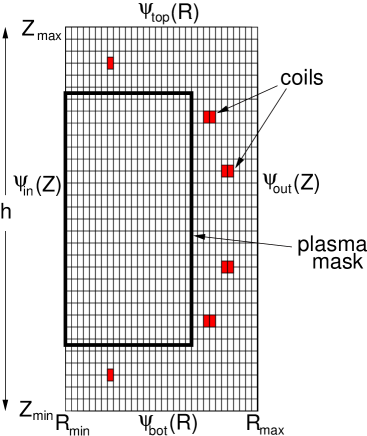
Figure 3: Schematic diagram of the computational domain used in the GRASS equilibrium solver, showing the main solution grid and the plasma mask.

The solver uses two rectangular grids:

1. The main solution grid, within the domain $(R_{\rm min},Z_{\rm min})$ to $(R_{\rm max},Z_{\rm max})$. The plasma and the coils are assumed to lie wholly within this grid. The poloidal flux values on the grid boundaries $\psi_{\rm in}$, $\psi_{\rm out}$, $\psi_{\rm top}$ and $\psi_{\rm bot}$ are calculated analytically from the given coil currents and an approximation to the current distribution in the plasma region.

2. The plasma mask, comprising the rectangular region $(R_{\rm p\,min},Z_{\rm p\,min})$ to $(R_{\rm p\,max},Z_{\rm p\,max})$. The mask must not extend outside the main solution grid. The (hot) plasma is assumed to lie wholly within the plasma mask, but no coils can be present inside it.

The coils’ current density $J_{c}$ (which needn’t be the same in each coil) is assigned to a number of grid cells, to approximate the coil locations and cross-section areas.

9.1.1 GRASS solution procedure

It is necessary to solve the following equation over the main solution grid:

$$\Delta^{*}\psi=\frac{4\pi}{c}RJ_{tor},$$

where $J_{tor}$ is a function of $\psi$ throughout the region containing plasma, and $J_{tor}=J_{c}$ at the coil locations. Thus we can rewrite the equation as

$$\Delta^{*}\psi=\frac{4\pi}{c}\left(RJ_{t}\,H+RJ_{c}\right),$$ (88)

where

$$H=\left\{\begin{array}[]{rl}1&\mbox{inside plasma mask}\\ 0&\mbox{elsewhere}\end{array}\right.$$

and $J_{t}$ is the toroidal component of $\mathbf{J}_{\mathbf{eq}}$ within the plasma:

$$RJ_{t}=-c\,R^{2}p^{\prime}-\frac{c}{4\pi}FF^{\prime}.$$ (89)

We denote by $E_{F}$ the toroidal electric field that drives the portion of the toroidal current density proportional to $-FF^{\prime}$. From the resistive MHD form of Ohm’s law we thus have

$$\frac{4\pi}{c}RJ_{t}=-4\pi\,R^{2}p^{\prime}+\frac{4\pi R}{c}\frac{E_{F}}{\eta}.$$

Setting $2\pi R\,E_{F}\equiv V_{F}$, the equivalent loop voltage, we obtain

$$RJ_{t}=-\frac{c\,R^{2}}{\Delta\psi}\frac{dp}{d\rho}+\frac{V_{F}^{*}}{\eta},$$ (90)

where $V_{F}^{*}=V_{F}/2\pi$ and $\Delta\psi=\psi_{\mbox{\scriptsize{edge}}}-\psi_{\mbox{\scriptsize{min}}}$ (see below). The dependencies of $dp/d\rho$ and $\eta$ on $\psi$ are prescribed.

To determine $V_{F}^{*}$ we divide Eq. (90) by $R$ and integrate over the poloidal cross-section area, identifying this quantity as the total plasma current $I_{p}$:

$$I_{p}\equiv\int J_{t}\,dA=-\int\frac{c\,R}{\Delta\psi}\frac{dp}{d\rho}\,dA+\int\frac{V_{F}^{*}}{R\,\eta}\,dA=-\frac{c}{\Delta\psi}\int R\frac{dp}{d\rho}\,dA+V_{F}^{*}\int\frac{dA}{R\,\eta}.$$

It follows from this that

$$V_{F}^{*}=\frac{I_{p}-\left(-\frac{c}{\Delta\psi}\int R\frac{dp}{d\rho}\,dA\right)}{\int\frac{dA}{R\,\eta}}.$$

It is convenient to introduce a new dependent variable $u=\psi/R^{1/2}$ satisfying the boundary conditions

$$u_{\rm in}(Z)=\frac{\psi_{\rm in}(Z)}{R_{\rm min}^{1/2}},\;\;\;u_{\rm out}(Z)=\frac{\psi_{\rm out}(Z)}{R_{\rm max}^{1/2}},$$

$$u_{\rm bot}(R)=\frac{\psi_{\rm bot}(R)}{R^{1/2}},\;\;\;u_{\rm top}(R)=\frac{\psi_{\rm top}(R)}{R^{\frac{1}{2}}}.$$

It is also convenient to express $\psi$ as the sum of two terms: $\psi_{1}$, which vanishes at $Z=Z_{\rm min}$ and $Z=Z_{\rm max}$; and

$$\psi_{2}\equiv\frac{Z-Z_{\rm min}}{h}\psi_{\rm top}+\frac{Z_{\rm max}-Z}{h}\psi_{\rm bot},$$

where $h=Z_{\rm max}-Z_{\rm min}$. The quantity $\psi_{1}$ is then equal to $\psi-\psi_{2}$. Equivalently,

$$u_{2}=\frac{Z-Z_{\rm min}}{h}u_{\rm top}+\frac{Z_{\rm max}-Z}{h}u_{\rm bot},$$

and $u_{1}\equiv u-u_{2}$. Clearly $u_{1}$ vanishes at $Z=Z_{\rm min}$ and $Z=Z_{\rm max}$, making it possible to compute this quantity by applying a sine Fourier transform in $Z$.

Defining the operator $\Delta^{*}_{u}$ by the equation

$$\Delta^{*}_{u}u\equiv\frac{1}{R^{1/2}}\Delta^{*}\psi=\frac{\partial^{2}u}{\partial R^{2}}+\frac{\partial^{2}u}{\partial Z^{2}}-\frac{3}{4R^{2}}u,$$

we find that the Grad-Shafranov equation becomes

$$\Delta^{*}_{u}u_{1}=\frac{\partial^{2}u_{1}}{\partial R^{2}}+\frac{\partial^{2}u_{1}}{\partial Z^{2}}-\frac{3}{4R^{2}}u_{1}=\frac{4\pi}{c}\left(\frac{RJ_{t}\,H}{R^{1/2}}+R^{1/2}J_{c}\right)-\Delta^{*}_{u}u_{2}.$$ (91)

Since $u_{2}$ is a prescribed function of $Z$, the quantity $\Delta^{*}_{u}u_{2}$ only needs to be evaluated once, at the beginning of the calculation. Moreover we can set $\Delta^{*}_{u}u_{2}=-3u_{2}/(4R^{2})$, since it is independent of $R$ and depends only linearly on $Z$.

We approach the problem of solving Eq. (91) by considering the parabolic equation

$$\frac{\partial u_{1}}{\partial\tau}=\epsilon\left(\Delta^{*}_{u}u_{1}-\alpha\right)$$ (92)

where $\alpha$ is the right hand side of Eq. (91), $\epsilon$ is a prescribed pseudo-conductivity (taken to be uniform across the poloidal plane) and $\tau$ is a fictitious, time-like iteration variable (not to be confused with the true time, $t$). The problem of solving Eq. (91) is thus equivalent to finding “steady-state” solutions of Eq. (92). The sine transform of Eq. (92) can be approximated by the finite difference equation

$$\frac{\hat{u}^{N+1}_{1\,i}-\hat{u}^{N}_{1\,i}}{\Delta\tau}=\epsilon\left[\frac{\hat{u}^{N+1}_{1\,i+1}-\hat{u}^{N+1}_{1\,i}}{(\Delta R)^{2}}-\frac{\hat{u}^{N+1}_{1\,i}-\hat{u}^{N+1}_{1\,i-1}}{(\Delta R)^{2}}-\frac{\pi^{2}k^{2}_{Z}}{h^{2}}\hat{u}^{N+1}_{1\,i}-\frac{3}{4R^{2}_{i}}\hat{u}^{N+1}_{1\,i}-\widehat{\alpha_{i}}\right],$$

where the $k_{Z}$-th sine transform coefficients are denoted by $\widehat{\ldots}$, $i$ labels the $i$-th grid point in the $R$ direction, with grid spacing $\Delta R$, $N$ labels the pseudo-time variable, and $\Delta\tau$ is the pseudo-time step. This equation can be rearranged to give

$$\hat{u}^{N+1}_{1\,i}\left(1+\Delta\tau\epsilon\left\{\frac{2}{(\Delta R)^{2}}+\frac{\pi^{2}k^{2}_{Z}}{h^{2}}+\frac{3}{4R^{2}_{i}}\right\}\right)-\frac{\Delta\tau\epsilon}{(\Delta R)^{2}}\hat{u}^{N+1}_{1\,i+1}-\frac{\Delta\tau\epsilon}{(\Delta R)^{2}}\hat{u}^{N+1}_{1\,i-1}=\hat{u}^{N}_{1\,i}-\Delta\tau\epsilon\,\widehat{\alpha_{i}},$$

which is a tridiagonal matrix equation of the form

$$\mathcal{A}_{i}\,\hat{u}^{N+1}_{1\,i-1}+\mathcal{B}_{i}\,\hat{u}^{N+1}_{1\,i}+\mathcal{C}_{i}\,\hat{u}^{N+1}_{1\,i+1}=\left(\hat{u}^{N}_{1\,i}-\Delta\tau\epsilon\,\widehat{\alpha_{i}}\right)$$

where

$$\mathcal{A}_{i}=-\frac{\Delta\tau\epsilon}{(\Delta R)^{2}},\;\;\;\;\;\mathcal{B}_{i}=1+\Delta\tau\epsilon\left\{\frac{2}{(\Delta R)^{2}}+\frac{\pi^{2}k^{2}_{Z}}{h^{2}}+\frac{3}{4R^{2}_{i}}\right\},\;\;\;\;\;\mathcal{C}_{i}=-\frac{\Delta\tau\epsilon}{(\Delta R)^{2}}.$$

The tridiagonal matrix equation is straightforward to solve for $\hat{u}^{N+1}_{1}$; the inverse sine transform of this yields $u_{1}$ and thereby $\psi_{1}$. The total flux $\psi$ is recovered by adding $\psi_{2}$, and the process is repeated until $\psi$ over the grid does not change significantly between pseudo-time steps.

9.1.2 Plasma current

In general the plasma current density $J_{t}$ and $\Delta\psi$ change between successive pseudo-time steps, and so the the evolution described by Eq. (92) is non-linear. It should be noted that the dependencies of $dp/d\rho$ and $\eta$ on $\psi$ (or $\rho$) are determined externally using CENTORI, rather than GRASS. Ideally these functions should vary with $\psi$ in such a way that the residual plasma current outside of the chosen edge plasma contour remains negligible.

9.1.3 Defining the plasma edge

Once a convergent solution for the equilibrium has been obtained, it is necessary to locate the edge of the plasma, which is defined to lie wholly within the plasma mask. By estimating $|\nabla\psi|$ at all grid points within the mask using finite differences, it is straightforward to find all the stationary points of $\psi$; these are either X-points (saddle points) or the magnetic axis, which is defined to lie at the global minimum of $\psi$ within the mask. There should be no other stationary points of $\psi$ inside the mask, unless some coils have been erroneously located within it. The edge of the plasma is then defined after finding a reference $\psi_{\rm max}$ using the following criteria (the situation is topologically more complicated in general, but in practice this algorithm suffices):

• If there are no X-points within the mask, $\psi_{\rm max}$ is chosen to be the minimum value of $\psi$ along the plasma mask perimeter or the minimum value of $\psi$ at a user-defined set of $(R,Z)$ “limiter” points within the mask, whichever is lower.

• If any X-points are present, $\psi_{\rm max}$ is chosen to be either the $\psi$ of the lowest X-point or the minimum value of $\psi$ along the inner or outer edges of the mask or the limiter points, if this is lower than the $\psi$ of the lowest X-point.

This ensures that the $\psi_{\rm max}$ contour is the largest closed contour within the mask. We then define the plasma edge contour $\psi_{\rm edge}$ to be

$$\psi_{\rm edge}=\psi_{\rm axis}+f(\psi_{\rm max}-\psi_{\rm axis}),$$

where $f=0.99$ when no X-points are present within the mask and $f=0.90$ otherwise. This has the effect of moving the effective plasma boundary to a contour lying slightly inside the last closed flux surface, which is necessary to ensure that the coordinate system described in Section 2 does not become strongly distorted near the plasma edge, and enables us to approximate the physics equations with central differences without incurring unacceptably large truncation errors.

Finally, $\psi$ is redefined within the plasma mask so that the plasma edge corresponds to $\psi=0$. CENTORI is passed only this modified $\psi(R,Z)$ within the masked region (thus excluding the coils), interpolated onto a grid of the same size (i.e. with the same number of elements) using Chebyshev fits in $R$ and $Z$. The algorithm for determining plasma-based coordinates described in Section 2 works extremely well when $\psi(R,Z)$ is specified in this way, and almost invariably yields a Jacobian $\mathcal{J}$ that closely approximates a flux function as a result.

9.1.4 Control of the magnetic axis location

It is sometimes useful to be able to hold the magnetic axis at a specified $(R,Z)$ position. For example, up-down asymmetric plasmas are often vertically unstable, and in such cases it may be difficult to obtain a convergent solution for the equilibrium using GRASS unless it is possible to control the plasma location during the convergence cycle.

Applying a vertical magnetic field makes it possible to control the radial position of the plasma, as follows. Suppose that there is a source of poloidal flux $\psi_{BZ}$ of the form

$$\psi_{BZ}=\psi_{BZ0}\,\frac{R^{2}}{R_{0}^{2}},$$

where $\psi_{BZ0}$ is a constant and $R_{0}$ is a measure of the major radius (e.g.the value of $R$ at the centre of the computational grid). Then

$$\nabla\psi_{BZ}=\frac{\partial\psi_{BZ}}{\partial R}\mathbf{e_{R}}=2R\frac{\psi_{BZ0}}{R_{0}^{2}}\mathbf{e_{R}}.$$

Since the poloidal magnetic field is $\nabla\zeta\times\nabla\psi$ it follows that the field due to $\psi_{BZ}$ is uniform and vertical:

$$\mathbf{B}_{Z}=\frac{2\psi_{BZ0}}{R_{0}^{2}}\mathbf{e_{Z}}.$$

The Lorentz force $\mathbf{J}_{\rm plas}\times\mathbf{B}_{Z}$ on the plasma arising from a positive plasma current $\mathbf{J}_{\rm plas}=J_{\rm plas}\,\mathbf{e_{\zeta}}$ will be inwards if $\psi_{BZ0}>0$.

Similarly, an externally-provided radial magnetic field affects the plasma’s vertical position. The radial field due to a poloidal flux of the form

$$\psi_{BR}=\psi_{BR0}\,\frac{Z-Z_{0}}{Z_{\rm max}-Z_{\rm min}},$$

is

$$\mathbf{B}_{R}=\frac{-\psi_{BR0}}{R(Z_{\rm max}-Z_{\rm min})}\mathbf{e_{R}},$$

and the Lorentz force on the plasma in this case is downwards if $\psi_{BR0}>0$ and $J_{\rm plas}>0$.

We adjust the values of $\psi_{BR0}$ and $\psi_{BZ0}$ during each GRASS convergence step by comparing the latest calculated position of the magnetic axis ($R_{\rm axis},Z_{\rm axis}$) with the target location ($R_{\rm target},Z_{\rm target}$), and applying a correction to the fluxes as follows:

$$\psi_{BR0}\rightarrow\psi_{BR0}+f\,\psi_{0}\,\frac{Z_{\rm axis}-Z_{\rm target}}{Z_{\rm max}-Z_{\rm min}},$$

$$\psi_{BZ0}\rightarrow\psi_{BZ0}+f\,\psi_{0}\,\frac{R_{\rm axis}-R_{\rm target}}{R_{target}},$$

where $f\ll 1$ (typically $f\sim 0.02$) to ensure that the change in the fluxes is not substantial. At $t=0$ we assume that $\psi_{BR0}=\psi_{BZ0}=0$. The applied corrections should modify the radial and vertical fields in such a way that the magnetic axis is pushed towards the target location.

It is important to note that the magnetic fields associated with these externally-applied poloidal flux components are curl-free and hence current-free, i.e. there are no additional current sources within the grid implied by their presence. Experimentally, vertical and radial magnetic field perturbations of this type can be introduced by changing the currents in poloidal field coils, although such field perturbations are in general non-uniform and therefore the uniform field perturbations discussed here are somewhat idealised. It is straightforward to incorporate the additional fluxes into GRASS by simply modifying the boundary conditions at the edge of the computational grid, at the start of each convergence loop, as follows:

$$u_{\rm in}(Z)=R_{\rm min}^{-1/2}\left(\psi_{\rm in}(Z)+\psi_{BR0}\frac{Z-Z_{0}}{Z_{\rm max}-Z_{\rm min}}+\psi_{BZ0}\frac{R_{\rm min}^{2}}{R_{0}^{2}}\right),$$

$$u_{\rm out}(Z)=R_{\rm max}^{-1/2}\left(\psi_{\rm out}(Z)+\psi_{BR0}\frac{Z-Z_{0}}{Z_{\rm max}-Z_{\rm min}}+\psi_{BZ0}\frac{R_{\rm max}^{2}}{R_{0}^{2}}\right),$$

$$u_{\rm bot}(R)=R^{-1/2}\left(\psi_{\rm bot}(R)+\psi_{BR0}\frac{Z_{\rm min}-Z_{0}}{Z_{\rm max}-Z_{\rm min}}+\psi_{BZ0}\frac{R^{2}}{R_{0}^{2}}\right),$$

$$u_{\rm top}(R)=R^{-1/2}\left(\psi_{\rm top}(R)+\psi_{BR0}\frac{Z_{\rm max}-Z_{0}}{Z_{\rm max}-Z_{\rm min}}+\psi_{BZ0}\frac{R^{2}}{R_{0}^{2}}\right).$$

10 Outline of code structure

10.1 Source files

The CENTORI code is written in standard Fortran 95 throughout, and is contained within some 21 source files. The bulk of these contain utility modules and routines to perform specific tasks such as I/O, parallel (MPI) communication, error handling, numerical evaluation (Chebyshev/Fourier fitting, and so on) and other customised but standard functionality. To make the code as portable as possible, we have avoided the use of external numerical libraries. Those areas of the code in which such libraries might improve performance almost all occur in non-parallel segments, i.e. are run only by the “global” processor. Since the execution of the code is overwhelmingly dominated by periods of parallel execution, serial optimisation through the use of specialised libraries is unlikely to confer significant benefits.

The physics within the code described in this paper is confined to two source files. One of these contains all the routines for initialising and evolving the physical fields, sources, sinks and so on, and also the routines for calculating plasma coordinates from the $\psi(R,Z)$ grid. The other contains the GRASS free boundary equilibrium solver as described in the previous section.

10.2 Parallelization model

CENTORI runs in parallel, with each MPI process advancing the physics quantities in an allocated three-dimensional subdomain. Aggregation of quantities such as flux surface or volume integrals and averages are performed across appropriate sections of the process population via specially-written routines. Halo-swapping is necessarily frequent due to the extensive calculation of derivatives. For the small grid sizes that are suitable for MAST simulations, there is a tendency for the parallelisation to become communication-limited for relatively low process counts. There are, however, two different implementations of the key numerical routines available, which are optimised for different local grid sizes [35]. Figure 4 shows speed-up versus process count for simulations performed on HECToR at EPCC and HPC-FF at the Jülich Supercomputing Centre when a computational grid of $129\times 65\times 33$ and the “eager” implementation of the key routines, which perform better for a large number of processes, are used. The HECToR results were obtained using the Phase 2b system, based on Cray’s XE6 hardware, which provides dual socket nodes with 2.1 GHz AMD Opteron 12-core processors and uses Cray’s proprietary Gemini Interconnect; the PGI compiler was used. The HPC-FF results were obtained using dual socket nodes with 2.93 GHz Intel Xeon X5570 quadcore processors and QDR Infiniband switch network; for these runs the Intel compiler was used. In this particular case the application shows almost linear speed-up for process numbers of up to 128, and continues to display a significant speed-up even for 512 processes. For a grid size of $129\times 129\times 129$ an almost linear speed-up is observed up to at least 512 processes (the largest number of processes used so far). Such a grid is larger than is normally used, but might be employed for ITER simulations in the future.

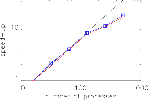
Figure 4: Execution time speed-up versus process count on HECToR (red with $+$ symbols) and HPC-FF (blue with $\Box$ symbols), relative to the time taken for a 16-process run, for a computational grid of $129\times 65\times 33$. This is the typical grid used for MAST simulations.

The computational domain is decomposed across the requested number of MPI processes in a standard Cartesian communicator, with periodicity automatically invoked in the two angular directions. Physics considerations suggest that the number of grid intervals $N_{\psi}$, $N_{\theta}$ and $N_{\zeta}$ in the radial, poloidal and toroidal directions should be roughly in the ratio $4:2:1$ (a benchmarking study has confirmed that this aspect ratio delivers results that are close to optimal [35]). In order to split each dimension into equal-sized portions across processes, the corresponding number of grid intervals must be one greater than a power of two, and the number of processes in each dimension must be an exact power of two. Thus, the computational grid used to model MAST typically has $N_{\psi}=129$, $N_{\theta}=65$, $N_{\zeta}=33$ over a corresponding grid of $8\times 4\times 4$ processes.

Novel techniques are used to optimise the serial execution (on each parallel process) of the numerical scheme within CENTORI. Specially designed derived datatypes employing advanced pointer techniques are used, together with lazy evaluation and the option to use strip-mining to tailor the code’s vectorisation. All the numerical vector operations (scalar and vector products, gradient, divergence and curl derivatives), and many pure scalar or combined scalar-vector operations, are contained within functional black boxes, hiding the implementation details of the underlying datatypes and the potential internal conversions between vector representations from the physics programmer. This enables a researcher to convert a complicated physics equation to a single line of code with ease. Full details are given in [35]. File handling is performed in parallel, with each process writing its own output data files. However an option is under development that uses MPI-IO routines to amalgamate the I/O more efficiently [36].

In contrast, the nature of the GRASS two-dimensional equilibrium solution over the entire poloidal cross-section of the plasma (and beyond) means that it is best performed in the $(R,Z)$ laboratory coordinates on a single process, as is the subsequent construction of the plasma coordinate system. This impacts only weakly on the code performance, as it is not necessary to recalculate the poloidal flux contours $\psi(R,Z)$ on timescales shorter than many microseconds, and thus GRASS is called only after many thousands of evolution timesteps; $\Delta t\sim 10^{-9}$ s is the typical timestep used. A typical run requires around 600 MB of RAM, and it takes around 12 hours on 128 MPI processes to simulate 1 ms of plasma evolution in typical tokamak conditions.

10.3 Additional features within the CENTORI package

The CENTORI code is best considered as a complete software package, rather than simply a collection of source and input files. In addition to its normal role for compilation, the makefile includes a number of utility functions that perform tasks such as automatic generation of the code documentation, and the creation of a tar file containing the entire source code, its documentation and visualisation files, and the input and output files. This has proved to be of great benefit in keeping all of the data from a given run together for archival purposes.

The source code is self-documenting to a degree, using an included parser program (autodoc) to generate html files for each subprogram from specially-formatted comment lines within the code. In addition, a full LaTeX manual is rigorously maintained to ensure its continued strict agreement with the evolving source code (this paper is an abridged version of the full manual).

A comprehensive visualisation suite has been developed to allow straightforward interpretation of the physics output from CENTORI. The program (CentoriScope) is written in the IDL language [37]. Work is in progress to bring CENTORI into the EU Integrated Tokamak Modelling (ITM [38]) framework.

The code is maintained within a private Subversion repository. Currently, access to the code is obtainable only by prior permission from the authors.

11 Example outputs

An early version of CENTORI was used to study wave propagation in the vicinity of magnetic X-points; analytical results for the evolution of perturbed wave energy and plasma kinetic energy in the ideal MHD limit were recovered numerically [39]. In this section we present two illustrative examples of calculations that can be performed using the full version of the code.

11.1 Tearing mode in large aspect ratio tokamak plasma

We demonstrate the capability of using CENTORI to model MHD instabilities by considering the example of a tearing mode in a very large aspect ratio (minor radius $a=0.36\,$m, major radius $R=16.8\,$m), circular cross-section tokamak plasma with a toroidal magnetic field of 9.7 T. For this purpose we prescribe an equilibrium with uniform density ($10^{24}\,$m^-3) and temperature ($T_{e}=T_{i}=46\,$eV). The resistivity, which we take to be given by the Spitzer expression [Eqs. (65) and (66)], is then equal to $3.67\times 10^{-16}\,$s, and the Lundquist number $S\equiv 4\pi av_{A}/(c^{2}\eta)\simeq 2\times 10^{4}$. The number of radial grid points (256) was chosen to be sufficiently large that the resistive layer width $d\sim aS^{-2/5}\simeq 0.7\,$cm was well-resolved. The quantity $FF^{\prime}$, which is proportional to the toroidal current density in this large aspect ratio limit, was prescribed to have the following profile:

$$FF^{\prime}={FF^{\prime}(0)\over\left\{1+\hbox{sinh}^{2}\left[2.09\rho\right]\right\}^{3/2}},$$ (93)

where $FF^{\prime}(0)$ is a constant, chosen to ensure that the corresponding $q$-profile remained above unity across the plasma, with $q=2$ at a normalised minor radius of about 0.65. This configuration is expected to be unstable to the growth of a tearing mode with poloidal and toroidal mode numbers $m=2$, $n=1$ [40]. For the purpose of this calculation only the generalised Ohm’s law and the ion momentum equation were used [Eqs. (36) and (37)]. Ohm’s law was reduced to the resistive MHD form, and viscosity was neglected in the momentum equation (except for the numerical viscosity described in Section 5.1.1, which is required to suppress numerical oscillations, but is set at a level which is sufficiently low for the system to be effectively inviscid). The electrostatic potential in this case was calculated not using Eq. (60) but by evolving the perpendicular ion velocity, identifying this as an ${\bf E}\times{\bf B}$ drift, and integrating to obtain $\Phi$. Nonlinear terms were omitted from both Ohm’s law and the momentum equation. Modes with $m/n$ equal to values of $q$ inside the plasma other than 2, such as the 3/2 mode, can also be unstable in the presence of a current density gradient; in general these modes cannot be exluded from simulations performed using a non-spectral code such as CENTORI. For this particular simulation, a Fourier filter was therefore applied at the end of each time step to exclude all harmonics other than the dominant 2/1 mode.

As expected, the configuration described above was found using CENTORI to be unstable to the growth of a 2/1 tearing mode. Figure 5 shows snapshots of $A_{\zeta}$ and $\Phi$ during the tearing mode growth. The profiles of these quantities resemble those obtained using CUTIE in a similar (although not identical) parameter regime; cf. Fig. 2 in Ref. [41], which was obtained with $S=2\times 10^{4}$ (defined in terms of the local resistivity at the magnetic axis) and relatively low viscosity (it should be noted that a precise comparison between tearing mode calculations performed using CENTORI and the CUTIE results presented in Ref. [41] is not in fact possible, since in the latter case a low aspect ratio ($R/a=2.5$) was assumed for the purpose of calculating the $q$-profile but the flux surfaces, as in all CUTIE simulations, were taken to be concentric circles; in a toroidal code such as CENTORI the circular flux surface limit can only be approached by taking the aspect ratio to be very large). The growth rate of the mode shown in Fig. 5 is approximately $2.5\times 10^{-3}/\tau_{A}$ where $\tau_{A}=a/v_{A}$ is the Alfvén time; this is comparable to the rate deduced analytically in Ref. [40], i.e. $\gamma\tau_{A}\sim S^{-3/5}$. It is somewhat lower than the rate found using CUTIE in the low viscosity limit with $S=2\times 10^{4}$ at the magnetic axis ($\gamma\tau_{A}\simeq 1.8\times 10^{-2}$) [41], but in this calculation the local resistivity at the $q=2$ surface was higher than the value at the magnetic axis, implying a higher 2/1 tearing mode growth rate.

Figure 5: Radial profiles of $A_{\zeta}$ (left) and $\Phi$ (right) in CENTORI simulation of tearing mode in large aspect ratio tokamak.

11.2 Turbulence simulation in conventional aspect ratio tokamak plasma

We present here the results of a CENTORI run simulating 1 ms of a conventional aspect ratio tokamak plasma with minor radius 0.55 m, major radius 1.67 m, elongation 1.7 and triangularity 0.18; the equilibrium flux surface contours, computed using GRASS, are shown in Fig. 6. The chosen plasma current was 1 MA, the toroidal magnetic field 2.5 T and the plasma volume 15 m³. The initial flux surface-averaged density, temperature and current density (primary quantities) were held approximately constant during the simulation by using adaptive sources of the form $S=-\alpha(\langle f\rangle-\langle f_{0}\rangle)$, where $f$ is the primary variable profile, $f_{0}$ is its initial profile, and $\alpha$ is an inverse reaction time response, set equal to the reciprocal of $\Delta t$, the CENTORI time step (0.5 ns, in this case). Both the initial ion velocity and the external momentum source $S_{v}$ were set equal to zero. The profiles of electron density, electron and ion temperatures, are shown in Fig. 7, together with the $q$-profile.

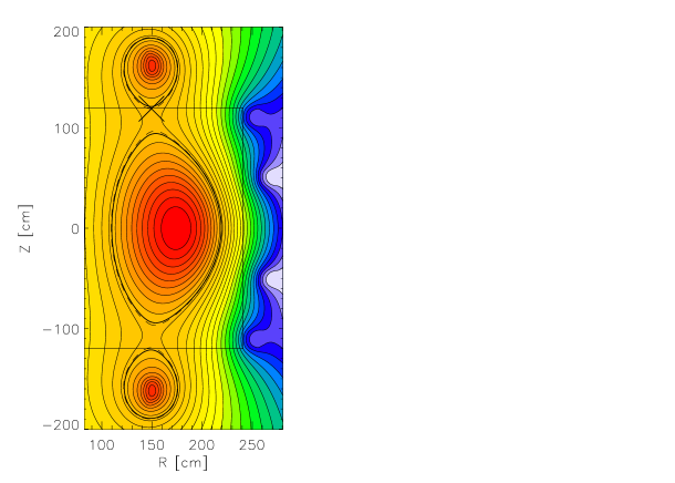
Figure 6: Plot of $\psi$ contours for plasma equilibrium used in turbulence simulation described in Section 11. The inner rectangle indicates the plasma mask used to construct this equilibrium; note that the boundary of the mask lies outside the region of confined plasma, bounded by a thick black curve.

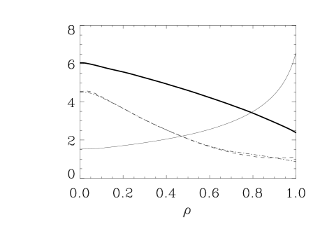
Figure 7: Profiles used in turbulence simulation described in Section 11. The thick solid curve shows the electron density in units of $10^{19}$m^-3, the thin solid curve is the $q$-profile, and the dashed and dashed-dotted curves show respectively the electron temperature and ion temperature in keV.

The evolution of the sources follows that of the fluctuations; after an initial transient, lasting around 100$\,\mu$s, they reached a quasi-steady level. The boundary conditions were those listed in Table 1. The spatial grid comprised 129 radial points, 65 poloidal points and 33 toroidal points. The run was executed on 64 processors of the HPC-FF machine at the Jülich Supercomputing Centre, the total wall-clock time being approximately 18 hours. Figure 8 shows the evolution of fluctuations in toroidal current density and electron density at $\rho=0.46$, $\theta=0$, $\zeta=0$. It is evident from a comparison of the relative amplitudes of the temporal variations in these two quantities that the fluctuations are electromagnetic in character.

Figure 8: Fluctuations in toroidal current density and electron density in outer midplane at $\rho=0.46$.

Figure 9 shows a poloidal cross-section of the toroidal current density fluctuations at $\zeta=0$. The $\times$ symbol in this figure marks the location chosen for the sample of local fluctuations shown in Fig. 8. The temporal evolution of the electron thermal conductivity is shown in Fig. 10. In the plasma turbulence literature this quantity is often normalised to the gyro-Bohm diffusivity $\chi_{\rm GB}=\rho_{s}^{2}c_{s}/L_{T}$ where $c_{s}=(T_{e}/m_{i})^{1/2}$, $\rho_{s}=c_{s}/\omega_{ci}$ and $L_{T}=T_{e}/(dT_{e}/dr)$ is the temperature scale length [42]. In the case of the local plasma parameters corresponding to the results shown in Fig. 10, $\rho_{s}^{2}c_{s}/L_{T}\simeq 12\,$m²s^-1; normalised to this value, the time-averaged thermal conductivity plotted in Fig. 10 is around 2, which is comparable to normalised $\chi_{e}$ values in gyro-kinetic simulations reported by Peeters and co-workers [42].

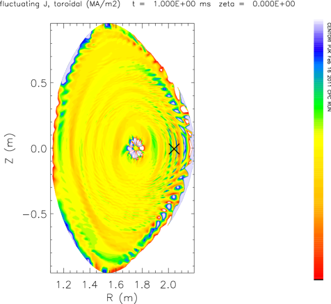
Figure 9: Contours of toroidal current density fluctuations in poloidal plane at $t=1\,$ms. The $\times$ symbol in the outer midplane indicates the approximate location corresponding to the results shown in Fig. 8.

Figure 10: Evolution of electron thermal conductivity in outer midplane at $\rho=0.46$.

The results presented above can be used to estimate the magnitudes of the potential and inductive contributions to the turbulent electric field; as noted in Section 5.1.1 only the potential electric field term is retained in the ion momentum equation in CENTORI. From Fig. 8 we note that the electron density fluctuations have a relative amplitude $\tilde{n}_{e}/n_{e}$ of the order of 10^-2. Electron force balance implies that the associated electrostatic potential fluctuations $\tilde{\Phi}$ are of order $10^{-2}T_{e}/e\sim 20\,$V, since the electron temperature at this point in the plasma is about 2 keV (cf. Fig. 7). Figure 9 indicates that the fluctuations have a characteristic scale length perpendicular to the magnetic field $L_{\perp}$ of order 10${}^{-2}\,$m, suggesting potential electric field fluctuations of $\tilde{\Phi}/L_{\perp}\sim 2\,$kVm^-1. In contrast, the frequency ($\omega\sim 200\,$krad s^-1) and amplitude ($\sim 0.03\,$MAm^-2) of the current fluctuations $\tilde{J}$ shown in the upper frame of Fig. 8 imply inductive electric fields of order $\omega\mu_{0}\tilde{J}L_{\perp}^{2}\sim 1\,$Vm^-1 ($\mu_{0}$ being the permeability of free space). Thus, for the parameters of this simulation (which are fairly representative of hot tokamak plasmas), the potential component of the fluctuating electric field is around three orders of magnitude larger than the inductive component, and our neglect of the latter in the ion momentum equation is therefore fully justified.

12 Conclusion

We have presented a comprehensive description of a novel two-fluid electromagnetic plasma turbulence code, CENTORI, together with sample output from a CENTORI simulation of a large aspect ratio tokamak plasma. The code is used to compute self-consistently the time evolution of plasma fluid quantities and fields in a toroidal configuration of arbitrary aspect ratio and plasma beta. The code is parallelised, and the equations are represented in fully finite difference form, ensuring good scalability. The equations are solved in a plasma coordinate system that is defined such that the Jacobian of the transformation from laboratory coordinates is a function only of the equilibrium poloidal flux, thereby accelerating vector operations and the evaluation of flux surface averages. GRASS, a subroutine of CENTORI, is used to determine the plasma equilibrium (and hence the plasma coordinates in which the fluid and Maxwell equations are solved) by computing the steady-state solutions of a diffusion equation with a pseudo-time derivative. The physics model implemented in CENTORI is based solidly on that used in the highly-successful CUTIE code, and we are confident that it will prove to be a powerful tool for the study of heat, particle and momentum transport in tokamak plasmas. In a forthcoming paper we will report the results of the first global simulations, performed using CENTORI, of electromagnetic, nonlinearly-saturated turbulence and transport in a spherical tokamak plasma (MAST).

References

- [1] M. Ottaviani and G. Manfredi, Nucl. Fusion 41 (2001) 637.
- [2] X. Garbet, C. Bourdelle, G.T. Hoang, P. Maget, S. Benkadda, P. Beyer, C. Figarella, I. Voitsekhovitch, O. Agullo, N. Bian, Phys. Plasmas 8 (2001) 2793.
- [3] T.T. Ribeiro, B.D. Scott, Plasma Phys. Control. Fusion 47 (2005) 1657.
- [4] B.D. Dudson, M.V. Umansky, X.Q. Xu, P.B. Snyder, H.R. Wilson, Comput. Phys. Comm. 180 (2009) 1467.
- [5] G.T.A. Huysmans, S. Pamela, E. van der Plas, P. Ramet, Plasma Phys. Control. Fusion 51 (2009) 124012.
- [6] A.H. Glasser, C.R. Sovinec, R.A. Nebel, T.A. Gianakon, S.J. Plimpton, M.A. Chu, D.D. Schnack, the NIMROD team, Plasma Phys. Control. Fusion 41 (1999) A747.
- [7] A.Y. Pankin, G. Bateman, D.P. Brennan, A.H. Kritz, S. Kruger, P.B. Snyder, C. Sovinec, the NIMROD team, Plasma Phys. Control. Fusion 49 (2007) S63.
- [8] C.R. Sovinec, T.A. Gianakon, E.D. Held, S.E. Kruger, D.D. Schnack, the NIMROD team, Phys. Plasmas 10 (2003) 1727.
- [9] H. Meyer et al., Nucl. Fusion 49 (2009) 104017.
- [10] F. Romanelli, R. Kamendje, Nucl. Fusion 49 (2009) 104006.
- [11] N. Holtkamp, Fusion Eng. Des. 82 (2007) 427.
- [12] W. Horton, D.-I. Choi, W.M. Tang, Phys. Fluids 24 (1981) 1077.
- [13] M. Romanelli, G. Regnoli, C. Bourdelle, Phys. Plasmas 14 (2007) 082305.
- [14] H. Sugama, Phys. Plasmas 7 (2000) 466.
- [15] K. G. McClements, L. C. Appel, M. J. Hole, A. Thyagaraja, Nucl. Fusion 42 (2002) 1155.
- [16] A. Thyagaraja, Plasma Phys. Control. Fusion 42 (2000) B255.
- [17] A. Thyagaraja, M. Valovič, P.J. Knight, Phys. Plasmas 17 (2010) 042507.
- [18] M. Abramowitz, I.A. Stegun, Handbook of Mathematical Functions, Dover, 1965, p. 795.
- [19] K.G. McClements, A. Thyagaraja A., Plasma Phys. Control. Fusion 53 (2011) 045009.
- [20] A.A. Ware, Phys. Rev. Lett. 25 (1970) 15
- [21] A.B. Rechester, M.N. Rosenbluth, Phys. Rev. Lett. 40 (1978) 38.
- [22] A. Thyagaraja, P.J. Knight and N. Loureiro, Eur. J. Mech. B/Fluids 23 (2004) 475.
- [23] A. Thyagaraja and K.G. McClements, Phys. Plasmas 13 (2006) 062502.
- [24] L. Spitzer, Astrophys. J. 116 (1952) 299.
- [25] J. Wesson, Tokamaks (3rd edition), Clarendon Press, Oxford, 2004, p.174.
- [26] C.S. Chang, F.L. Hinton, Phys. Fluids 25 (1982) 1493.
- [27] F.L. Hinton, R.D. Hazeltine, Rev. Mod. Phys. 48 (1976) 239.
- [28] R.J. Akers, P. Helander, A. Field, C. Brickley, D. Muir, N.J. Conway, M. Wisse, A. Kirk, A. Patel, A. Thyagaraja, C.M. Roach, the MAST and NBI Teams, Proceedings of the 20th IAEA Fusion Energy Conference, International Atomic Energy Agency, Vienna, 2005, EX/4-4.
- [29] R. Stoll, F. Porté-Agel, Boundary-Layer Meteorology 126 (2008) 1.
- [30] C.A.J. Fletcher, Computational Techniques for Fluid Dynamics 1: Fundamental and General Techniques (2nd edition), Springer-Verlag, Berlin, 1991, p.208.
- [31] E. Hameiri, Phys. Fluids 26 (1983) 230.
- [32] S. Migliuolo, A. K. Sen, Phys. Fluids B 2 (1990) 3047.
- [33] I.T. Chapman, N.R. Walkden, J.P. Graves, C. Wahlberg, Plasma Phys. Control. Fusion 53 (2011) 125002.
- [34] A. Thyagaraja, P.J. Knight, A novel solution method for tokamak plasma force balance, in Progress in Industrial Mathematics at ECMI 2008, Springer-Verlag, Berlin, 2010, p. 1047.
- [35] T.D. Edwards, Optimising a fluid plasma turbulence code on modern high performance computers, PhD Thesis, University of Edinburgh, 2010.
- [36] G. Huhs, CENTORI - Installation, Performance, and Enhancements, Barcelona Supercomputing Center Technical Report TR/CASE-10-1, 2010, http://www.bsc.es/media/4367.pdf
- [37] ITT Visual Information Solutions, http://www.ittvis.com
- [38] EFDA Task Force Integrated Tokamak Modelling, https:/www.efda-itm.eu
- [39] K.G. McClements, A. Thyagaraja, P.J. Knight, N. Ben Ayed, L. Fletcher, Proceedings of the 31st EPS Conference on Plasma Physics, London, 28 June - 2 July 2004, ECA Vol.28B, P-5.061 (2004).
- [40] H.P. Furth, J. Killeen, M.N. Rosenbluth Phys. Fluids 6 (1963) 459.
- [41] A. Thyagaraja, Plasma Phys. Control. Fusion 36 (1994) 1037.
- [42] A.G. Peeters, Y. Camenen, F.J. Casson, W.A. Hornsby, A.P. Snodin, D. Strintzi, G. Szepesi, Comput. Phys. Comm. 180 (2009) 2650.