The Complexity of Approximating a Bethe Equilibrium

Abstract

This paper resolves a common complexity issue in the Bethe approximation of statistical physics and the Belief Propagation (BP) algorithm of artificial intelligence. The Bethe approximation and the BP algorithm are heuristic methods for estimating the partition function and marginal probabilities in graphical models, respectively. The computational complexity of the Bethe approximation is decided by the number of operations required to solve a set of non-linear equations, the so-called Bethe equation. Although the BP algorithm was inspired and developed independently, Yedidia, Freeman and Weiss (2004) showed that the BP algorithm solves the Bethe equation if it converges (however, it often does not). This naturally motivates the following question to understand limitations and empirical successes of the Bethe and BP methods: is the Bethe equation computationally easy to solve?

We present a message-passing algorithm solving the Bethe equation in a polynomial number of operations for general binary graphical models of $n$ variables where the maximum degree in the underlying graph is $O(\log n)$. Our algorithm can be used as an alternative to BP fixing its convergence issue and is the first fully polynomial-time approximation scheme for the BP fixed-point computation in such a large class of graphical models, while the approximate fixed-point computation is known to be (PPAD-)hard in general. We believe that our technique is of broader interest to understand the computational complexity of the cavity method in statistical physics.

1 Introduction

In recent years, graphical models (also known as Markov random fields) defined on graphs have been studied as powerful formalisms modeling inference problems in numerous areas including computer vision, speech recognition, error-correcting codes, protein structure, networking, statistical physics, game theory and combinatorial optimization. Two central problems, commonly addressed in these applications involving graphical models, are computing the marginal distribution and the so-called partition function. It is well-known that inference problems are computationally hard in general [5]. Due to such a theoretical barrier, efforts have been made to develop heuristic methods.

The sum-product algorithm, also known as Belief Propagation (BP), and its variants (e.g., Survey Propagation) are such heuristics, driven by certain experimental thoughts, for computing the marginal distribution, where BP was first proposed by Gallager [12] for error correcting codes and Pearl [20] for artificial intelligence. Their appeal lies in the ease of implementation as well as optimality in tree-structured graphical models (models which contain no cycles). BP (and message-passing algorithms in general) can be thought as an updating rule on a set of messages:

$$m^{t+1}~{}:=~{}f\left(m^{t}\right),$$

where $m^{t}$ is the multi-dimensional vector of messages at the $t$-th iteration, and $f$ describes the updating rule (or BP operator). Two major hurdles to understand such a message-passing algorithm are its convergence (i.e., does $m^{t}$ converge to $m^{*}$?) and correctness (i.e., is $m^{*}$ good enough?). It is known that the BP iterative procedure always has a fixed-point $m^{*}$ due to the Brouwer’s fixed-point theorem. However, BP can oscillate far from a fixed-point in models with cycles, and only sufficient convergence conditions [28, 24, 14, 15] have been established in the last decade. More importantly, BP can have multiple fixed-points, and even when the fixed-point is unique, it may not be the correct answer. Significant efforts [14, 27, 29] were made to understand BP fixed-points, while the precise approximation qualities and the rigorous understandings on their limitations still remain a mystery. Regardless of those theoretical understandings, the BP algorithm performs empirically well in many applications [11, 19]. For example, the highly successful turbo decoding algorithm [3] can be interpreted as BP [18] and decisions guided by BP are also known to work well to solve satisfiability problems [21].

The Bethe approximation [2, 29] and its variants (e.g., Kikuchi approximation [9]), originally developed in statistical physics of lattice models, are currently used as powerful approximation schemes for computing the (logarithm of the) partition function in many applications. The Bethe approximation suggests to use the following quantity as an approximation for the logarithm of the partition function:

$$\qquad\qquad\qquad\qquad\qquad\qquad\qquad F(\mathbf{y}^{*})\qquad\qquad\qquad\mbox{where}\quad\nabla F(\mathbf{y}^{*})=0.$$

Here, $F$, $\nabla F(\mathbf{y}^{*})=0$ and $\mathbf{y}^{*}$ are called the (minus) Bethe free energy function, Bethe equation and Bethe equilibrium, respectively. The statistical physics prediction suggests its asymptotic correctness in random sparse graphical models, and several rigorous evidences in particular models are known [1, 8, 4]. Efforts have also been made to estimate and characterize its error [6, 22, 23]. However, the error still remains uncontrollable for models with many cycles.

Yedidia, Freeman and Weiss [29] established a somewhat surprising connection between the BP algorithm and the Bethe approximation: if BP converges, it solves the Bethe equation. Equivalently, the BP fixed-point equation $f(m^{*})=m^{*}$ is in essence equivalent to the Bethe equation $\nabla F(\mathbf{y}^{*})=0$. This naturally leads to the following common computational question for both: is the BP fixed-point computation computationally easy? Formally speaking,

• Given $\varepsilon>0$, is it possible to design a deterministic iterative algorithm finding $m^{*}$ satisfying

  $$(1-\varepsilon)\,f(m^{*})~{}\leq~{}{m^{*}}~{}\leq~{}(1+\varepsilon)\,f(m^{*}),$$

  in a polynomial number of bitwise operations with respect to $1/\varepsilon$ and the dimension of the vector $m^{*}$?

Such an algorithm can be used as an alternative to BP with provably fast convergence rate (i.e., fixing the convergence issue of BP) and eliminates a need for the convergence analysis of BP. Even though it may not converge to the precise answer, rough estimations on marginal probabilities are sometimes enough to solve hard computational problems (see [21], for example). Further, it justifies that the Bethe approximation is a polynomial-time scheme since $m^{*}$ satisfying the above inequality provides $\mathbf{y}^{*}$ with $\|\nabla F(\mathbf{y}^{*})\|\leq\varepsilon$. Efforts to design such algorithms were made [25, 30], but no rigorous analysis on their convergence rates is known. The authors in [4] provide an algorithm with provable polynomial convergence rate, but the work is for a very specific graphical model (i.e., the uniform distribution on independent sets of sparse graphs). It is far from being clear whether such a poly-convergence algorithm exists for more general graphical models. This is primarily because the Bethe function is usually neither convex nor concave (cf., [26]) and computing a local minimum (or a fixed-point) approximately are known to be believably (PPAD- or PLS-)hard in general [7].

1.1 Our Contribution

The main result of this paper is the following answer $\mathcal{A}$ (see Theorem 2 in Section 3) for the question $\mathcal{Q}$ for the BP operator $f$ and general sparse binary graphical models of which potential functions are bounded above and below by some positive constants. To state it formally, we let $n$ be the number of nodes and $\Delta$ be the maximum degree in the underlying graph, respectively.

• Given $\varepsilon>0$, there exists a deterministic iterative algorithm finding $m^{*}$ satisfying

  $$(1-\varepsilon)\,f(m^{*})~{}\leq~{}{m^{*}}~{}\leq~{}(1+\varepsilon)\,f(m^{*})$$

  in $2^{O(\Delta)}n^{2}\varepsilon^{-4}\log^{3}(n\varepsilon^{-1})$ iterations.

In this paper, we call the message $m^{*}$ satisfying the above inequality an $\varepsilon$-approximate BP fixed-point. In what follows, we explain the algorithm in details.

The known equivalence [29] between the BP fixed-point equation and the Bethe equation implies that the question $\mathcal{Q}$ is equivalent to the following.

• Given $\varepsilon^{\prime}>0$, is it possible to design a deterministic iterative algorithm finding $\mathbf{y}^{*}$ satisfying

  $$\|\nabla F(\mathbf{y}^{*})\|~{}\leq~{}\varepsilon^{\prime},$$

  in a polynomial number of bitwise operations with respect to $1/\varepsilon^{\prime}$ and the dimension of the domain $D$ of the Bethe free energy function $F$?

However, we remind the reader that it is still far from being obvious whether it is computationally ‘easy’ to find such a near-stationary point or an approximate local minimum (or maximum). Natural attempts are gradient-descent algorithms to find a local minimum or maximum of $F$: iteratively update $\mathbf{y}(t)$ as

$$\mathbf{y}(t+1)~{}:=~{}\mathbf{y}(t)+\alpha\,\nabla F(\mathbf{y}(t)),$$

where $\alpha\in\mathbb{R}$ is the (appropriately chosen) step-size. The main issue here is that the gradient-descent algorithm may not find a near-stationary point if $\mathbf{y}(t)$ hits the boundary of $D$ in one of its iterations (and a projection is required). Hence, the main strategy in [4] to avoid the hitting issue lies in (a) understanding the behavior of the gradient $\nabla F$ close to the boundary of $D$ and (b) designing an appropriate small step-size in the gradient-descent algorithm based on the understanding (a).

Now we give an overview of our technical contributions. The main challenge to apply the strategy to general binary graphical models (beyond the specific model in [4]) is on (a). The main observation used in [4] is that the domain $D$ can be reduced to $\left[0,\frac{1}{2}\right]^{n}$ in the uniform independent-set model. In general, the dimension of $D$ is is much larger than $n$ (i.e., the number of nodes) since the parameter $\mathbf{y}$ of the Bethe function $F$ represents not only node marginal probabilities but also edge (i.e., pairwise) ones. However, in independent-set models, pairwise marginal probabilities are decided by node marginal probabilities, which allows to reduce the dimension of $D$ to $n$. The proof strategy in [4] crucially relies on $D=\left[0,\frac{1}{2}\right]^{n}$ and immediately fails even for a non-uniform independent-set model whose domain $D$ is reduced to $[0,1]^{n}\not\subset\left[0,\frac{1}{2}\right]^{n}$. Furthermore, in general binary graphical models, such a dimension reduction in $D$ is impossible and it is not hard to check that any similar approaches with [4] fail without it. To overcome such a technical issue, we first observe that at stationary points of $F$, pairwise marginal probabilities should satisfy certain quadratic equations in terms of node marginal probabilities in binary graphical models. Hence, one can express the Bethe free energy again in terms of node marginal probabilities (i.e., a dimension reduction in $D$ is possible) for the purpose of obtaining a (near-)stationary point of $F$. Now we study this ‘modified’ Bethe expression $F^{*}$ to avoid the hitting issue, which we end up with an appropriate small step-size in the gradient-descent algorithm. Moreover, we eliminate a need to decide such a small step-size explicitly in the algorithm, by designing a time-varying projection scheme.

We later realize that the ‘modified’ Bethe expression $F^{*}$ was already proposed by Teh and Welling [25], where they suggested gradient algorithms to minimize $F^{*}$ using sigmoid functions. The main difference in our work is that we study the behavior of the gradient $\nabla F^{*}$ close to the boundary of its domain and guarantee that the gradient-descent algorithm does not hit the boundary of the underlying domain $D$, i.e., we do not use sigmoid functions. The success of our rigorous convergence rate analysis, which was missing in the work of Teh and Welling (2001), primarily relies on this difference. It is also crucial to extend the algorithm design to non-binary graphical models as we describe in Section 4.

One can observe that our gradient-descent algorithm is implementable as a ‘BP-like’ iterative, message-passing algorithm: each node maintains a message at each iteration and passes it to its neighbors. If potential functions in binary graphical models are bounded above and below by some positive constants (i.e., their values are $\Theta(1)$), we prove it terminates in $2^{O(\Delta)}n^{2}\varepsilon^{-4}\log^{3}(n\varepsilon^{-1})$ iterations until it finds an $\varepsilon$-approximate BP fixed-point (see Theorem 2 in Section 3). In a complexity point of view, the only remaining issue is that each node may require to maintain irrational messages (of infinitely long bits). We further show that a polynomial number (with respect to $1/\varepsilon$, $n$ and $2^{\Delta}$) of bits to approximate each message suffices, and hence the algorithm consists of only a polynomial number of bitwise operations in total. Namely, it is a fully polynomial-time approximation scheme (FPTAS) to compute an approximate BP fixed-point for sparse binary graphical models where $\Delta=O(\log n)$. Finally, we note that our ‘quadratic’ running-time guarantee (i.e., $2^{O(\Delta)}n^{2}\varepsilon^{-4}\log^{3}(n\varepsilon^{-1})$) is merely a theoretical bound, and far from being tight. In our experimental results reported in Section 5, we observe that our algorithm sometimes converges faster than the standard BP algorithm.

1.2 Organization

In Section 2, we provide backgrounds for graphical models, Belief Propagation and Bethe approximation. In Section 3, we describe our algorithm and its time complexity for binary graphical models. In Section 4, we discuss, at a high level, how to extend the result to non-binary graphical models. From our discussion in Section 4, one can observe that it is not hard to obtain the similar convergence rate result for such graphical models as well. But, we omit the further details in this paper. Experimental results are reported in Section 5.

2 Graphical Models

We first introduce a class of joint distributions defined with respect to (undirected) graphs, which are called pairwise Markov random fields (MRFs) [17]. Specifically, let $G=(V,E)$ be an undirected graph with vertex set V where $|V|=n$, and edge set $E\subseteq{V\choose 2}$ denoting a set of unordered pairs of vertices. The vertices of $G$ label a collection of random variables $\mathbf{x}=\{x_{v}\,|\,v\in V\}$. Our primary focus in this paper is on binary random variables, i.e., $x_{v}\in\{0,1\}$ for all $v\in V$.

Now consider the following joint distribution on $\{0,1\}^{n}$ that factors according to $G$:

$$p(\mathbf{x})=\frac{1}{Z}\prod_{v\in V}\psi_{v}(x_{v})\prod_{(u,v)\in E}\psi_{u,v}(x_{u},x_{v})\qquad\mbox{for}~{}~{}\mathbf{x}\in\{0,1\}^{n}.$$

Here, $\psi_{u,v}$ for $(u,v)\in E$ and $\psi_{v}$ for $v\in V$ are non-negative functions on $\{0,1\}^{2}$ and $\{0,1\}$, respectively. These local functions are called potential functions or compatibility functions. The normalizing factor $Z$ is called the partition function:

$$Z=\sum_{\mathbf{x}\in\{0,1\}^{n}}\prod_{v\in V}\psi_{v}(x_{v})\prod_{(u,v)\in E}\psi_{u,v}(x_{u},x_{v}).$$ (1)

Finally, some notations. Let $\mathcal{N}(v)$ be the set of neighbors of a vertex $v\in V$, $d_{v}:=|\mathcal{N}(v)|$ be the degree of $v\in V$, and $\Delta:=\max_{v}d_{v}$ be the maximum degree in the graph $G$. Further, we define

$$|\psi|~{}:=~{}\max_{(u,v)\in E,x_{u},x_{v}\in\{0,1\}}\left\{e^{|\ln\psi_{v}(x_{v})|},e^{|\ln\psi_{u,v}(x_{u},x_{v})|}\right\}.$$

We primarily focus on the case $|\psi|<\infty$, which excludes the case $\psi_{u,v}(\cdot,\cdot)=0$. However, this does not hurt the generality of the results in this paper too much since one can consider tiny perturbations to such ‘zero’ potential functions so that the distribution remains almost the same.

2.1 Belief Propagation

The BP algorithm has messages $\{m^{t}_{u\rightarrow v}(\cdot),m^{t}_{v\rightarrow u}(\cdot)\}:=\{m^{t}_{u\rightarrow v}(x_{v}),m^{t}_{v\rightarrow u}(x_{u}):(u,v)\in E,x_{v},x_{u}\in\{0,1\}\}$ at the $t$-th iteration and it updates them as

$$m^{t+1}_{u\to v}(x_{v}) \propto \sum_{x_{u}\in\{0,1\}}\psi_{u,v}(x_{u},x_{v})\psi_{u}(x_{u})\prod_{w\in\mathcal{N}(u)\backslash v}m^{t}_{w\to u}(x_{u}),$$

where $\sum_{x_{v}\in\{0,1\}}m^{t+1}_{u\to v}(x_{v})=1$. This is equivalent to the following updating rule on (reduced) messages $\{m^{t}_{u\to v},m^{t}_{v\rightarrow u}\}$.

$$m^{t+1}_{u\to v} := f_{u\rightarrow v}\left(\prod_{w\in\mathcal{N}(u)\backslash v}m^{t}_{w\to u}\right),$$

where $m^{t}_{u\to v}:=m^{t}_{u\to v}(1)/m^{t}_{u\to v}(0)$ and the function $f_{u\rightarrow v}:\mathbb{R}_{+}\to\mathbb{R}_{+}$ is defined as

$$f_{u\rightarrow v}(x)~{}:=~{}\frac{\psi_{u,v}(0,1)\psi_{u}(0)+\psi_{u,v}(1,1)\psi_{u}(1)\cdot x}{\psi_{u,v}(0,0)\psi_{u}(0)+\psi_{u,v}(1,0)\psi_{u}(1)\cdot x}.$$

The initial messages at the first iteration can be chosen arbitrarily as positive real numbers, where the standard choice is $m^{1}_{u\to v}=m^{1}_{v\to u}=1$ for all $(u,v)\in E$.

Now the BP fixed-point of messages $\{m_{u\rightarrow v},m_{v\rightarrow u}\}$ can be naturally defined as

$$m_{u\to v}~{}=~{}f_{u\rightarrow v}\left(\prod_{w\in\mathcal{N}(u)\backslash v}m_{w\to u}\right),\qquad\forall~{}(u,v)\in E.$$ (2)

If $|\psi|<\infty$, one can easily argue the existence of such a (finite) fixed-point using the Brouwer’s fixed-point theorem. This motivates the following notion of $\varepsilon$-approximate BP fixed-point.

Definition 1.

The set of messages $\{m_{u\rightarrow v},m_{v\rightarrow u}:(u,v)\in E\}$ is called an $\varepsilon$-approximate BP fixed-point if

$$\left|\frac{m_{u\to v}}{f_{u\rightarrow v}\left(\prod_{w\in\mathcal{N}(u)\backslash v}m_{w\to u}\right)}-1\right|~{}\leq~{}\varepsilon,\qquad\forall~{}(u,v)\in E.$$ (3)

The BP estimates for node and edge marginal probabilities based on messages, denoted by $\tau_{v}(\cdot),\tau_{u,v}(\cdot)$ for $v\in V,(u,v)\in E$, are defined as

$$\tau_{v}(x_{v}) \propto \psi_{v}(x_{v})\prod_{u\in\mathcal{N}(v)}m_{u\to v}(x_{v})$$

$$\tau_{u,v}(x_{u},x_{v}) \propto \psi_{u}(x_{u})\psi_{v}(x_{v})\psi_{u,v}(x_{u},x_{v})\left(\prod_{w\in\mathcal{N}(u)\setminus v}m_{w\to u}(x_{u})\right)\left(\prod_{w\in\mathcal{N}(v)\setminus u}m_{w\to v}(x_{v})\right),$$

where $\sum_{x_{v}}\tau_{v}(x_{v})=1$ and $\tau_{v}(x_{v})=\sum_{x_{u}}\tau_{u,v}(x_{u},x_{v})$.

2.2 Bethe Approximation

The Bethe approximation [29] is an approximation to the logarithm of the partition function (i.e., $\ln Z$), given by

$$\sum_{v\in V}\sum_{x_{v}}\tau_{v}(x_{v})\left[\ln\psi_{v}(x_{v})-\ln\tau_{v}(x_{v})\right]+\sum_{\{u,v\}\in E}\sum_{x_{u},x_{v}}\tau_{u,v}(x_{u},x_{v})\Bigg{[}\ln\psi_{u,v}(x_{u},x_{v})-\ln\frac{\tau_{u,v}(x_{u},x_{v})}{\tau_{u}(x_{u})\tau_{v}(x_{v})}\Bigg{]},$$

where $\tau_{v}(\cdot),\tau_{u,v}(\cdot)$ are marginal estimates at a BP fixed-point. Under the constraints $\sum_{x_{v}}\tau_{v}(x_{v})=1$ for all $v\in V$ and $\tau_{v}(x_{v})=\sum_{x_{u}}\tau_{u,v}(x_{u},x_{v})$ for all $v\in V,x_{v}\in\{0,1\}$, this expression can be written as a function of $\mathbf{y}=[y_{v},y_{u,v}]$ where $y_{v}=\tau_{v}(1)$ and $y_{u,v}=\tau_{u,v}(1,1)$.

$$F(\mathbf{y}) := \sum_{v\in V}y_{v}(\ln\psi_{v}(1)-\ln y_{v})+(1-y_{v})(\ln\psi_{v}(0)-\ln(1-y_{v}))$$ (4)

$$\qquad+\sum_{(u,v)\in E}\Bigg{[}(1-y_{u}-y_{v}+y_{u,v})\left(\ln\psi_{u,v}(0,0)-\ln\frac{1-y_{u}-y_{v}+y_{u,v}}{(1-y_{u})(1-y_{v})}\right)$$

$$\qquad\qquad\qquad\qquad+(y_{u}-y_{u,v})\left(\ln\psi_{u,v}(1,0)-\ln\frac{y_{u}-y_{u,v}}{y_{u}(1-y_{v})}\right)$$

$$\qquad\qquad\qquad\qquad+(y_{v}-y_{u,v})\left(\ln\psi_{u,v}(0,1)-\ln\frac{y_{v}-y_{u,v}}{(1-y_{u})y_{v}}\right)$$

$$\qquad\qquad\qquad\qquad+y_{u,v}\left(\ln\psi_{u,v}(1,1)-\ln\frac{y_{u,v}}{y_{u}y_{v}}\right)\Bigg{]},$$

where $-F$ is called the Bethe free energy function [29]. The gradient $\nabla F(\mathbf{y})=\left[\frac{\partial F}{\partial y_{v}},\frac{\partial F}{\partial y_{u,v}}\right]$ can be obtained as

$$\frac{\partial F}{\partial y_{v}} = \Psi^{(v)}+\ln\frac{1-y_{v}}{y_{v}}+\sum_{u\in\mathcal{N}(v)}\ln\left(\frac{1-y_{v}-y_{u}+y_{u,v}}{1-y_{v}}\cdot\frac{y_{v}}{y_{v}-y_{u,v}}\right)$$ (5)

$$\frac{\partial F}{\partial y_{u,v}} = \Psi^{(u,v)}+\ln\left(\frac{y_{u}-y_{u,v}}{1-y_{u}-y_{v}+y_{u,v}}\cdot\frac{y_{v}-y_{u,v}}{y_{u,v}}\right),$$ (6)

where

$$\Psi^{(v)}:=\ln\frac{\psi_{v}(1)}{\psi_{v}(0)}+\sum_{u\in\mathcal{N}(v)}\ln\frac{\psi_{u,v}(0,1)}{\psi_{u,v}(0,0)}\qquad\mbox{and}\qquad\Psi^{(u,v)}:=\ln\frac{\psi_{u,v}(0,0)\,\psi_{u,v}(1,1)}{\psi_{u,v}(1,0)\,\psi_{u,v}(0,1)}.$$ (7)

It is known that there is a one-to-one correspondence between BP fixed-points and zero gradient points of $F$. In particular, one can obtain the following lemma whose proof can be done easily using the algebraic expressions (5) and (6) of gradients.

Lemma 1.

Given $\varepsilon\in[0,1)$, suppose $\mathbf{y}=[y_{v},y_{u,v}]$ satisfies $\|\nabla F(\mathbf{y})\|_{\infty}\leq\varepsilon$. Then, the set of messages $\{m_{u\rightarrow v},m_{v\rightarrow u}:(u,v)\in E\}$ is a $6\varepsilon$-approximate BP fixed-point if it is given as

$${m_{u\to v}}=\frac{\psi_{u,v}(0,1)}{\psi_{u,v}(0,0)}\cdot\frac{1-y_{v}-y_{u}+y_{u,v}}{1-y_{v}}\cdot\frac{y_{v}}{y_{v}-y_{u,v}}.$$ (8)

The proof of Lemma 1 is presented in Appendix A. For somewhat ‘non-intuitive’ formula (8), we also provide some intuition in Appendix B.

3 Algorithm for Computing BP Fixed-Points

In this section, we present the main result of this paper, a new message-passing algorithm for approximating a BP fixed-point. From the (algebraic) relationship between approximate BP fixed-points and near-stationary points of the Bethe free energy function $F$ in Lemma 1, it is equivalent to compute a near-stationary point $\mathbf{y}$, i.e., $\|\nabla F(\mathbf{y})\|_{2}\leq\varepsilon$.

Our algorithm, described next, for finding such a point is essentially motivated by the standard (projected) gradient-descent algorithm. The non-triviality (and novelty) lies in our choice of an appropriate (time-varying) ‘projection $[\cdot]_{*}$’ with respect to the (time-varying) ‘step-size $\frac{1}{\sqrt{t}}$’ at each iteration and subsequent analysis of the rate of convergence.

Algorithm A  

• Algorithm parameters:

  $$\varepsilon\in(0,1)\qquad\mbox{and}\qquad\mathbf{y}_{V}(t)=\left[\,y_{v}(t)\in(0,1):v\in V\,\right]\quad\mbox{at the $t$-th iteration.}$$

  Initially, $y_{v}(1)=1/2$ for all $v\in V$.

• $\mathbf{y}_{V}(t)$ is updated as:

  $$y_{v}(t+1) = \Bigg{[}y_{v}(t)+\frac{1}{\sqrt{t}}\Bigg{(}\Psi^{(v)}+\ln\frac{1-y_{v}(t)}{y_{v}(t)}$$

  $$\qquad\qquad\qquad+\sum_{u\in\mathcal{N}(v)}\ln\left(\frac{1-y_{v}(t)-y_{u}(t)+y_{u,v}(t)}{1-y_{v}(t)}\cdot\frac{y_{v}(t)}{y_{v}(t)-y_{u,v}(t)}\right)\Bigg{)}\Bigg{]}_{*},$$

  where the projection $[\cdot]_{*}$ at the $t$-th iteration is defined as

  $$[x]_{*}:=\begin{cases}x&\mbox{if}~{}\frac{0.1}{t^{1/4}}\leq x\leq 1-\frac{0.1}{t^{1/4}}\\ \frac{0.1}{t^{1/4}}&\mbox{if}~{}x<\frac{0.1}{t^{1/4}}\\ 1-\frac{0.1}{t^{1/4}}&\mbox{if}~{}x>1-\frac{0.1}{t^{1/4}}\end{cases},$$

  and $y_{u,v}(t)>0$ is computed as the unique solution satisfying

  $$e^{\Psi^{(u,v)}}\cdot\frac{y_{u}(t)-y_{u,v}(t)}{1-y_{u}(t)-y_{v}(t)+y_{u,v}(t)}\cdot\frac{y_{v}(t)-y_{u,v}(t)}{y_{u,v}(t)}=1\quad\mbox{and}\quad y_{u,v}(t)<\min\{y_{v}(t),y_{u}(t)\}.$$

• Compute messages $\{m_{u\rightarrow v},m_{v\rightarrow u}\}$ as

  $$m_{u\to v}~{}=~{}\frac{\psi_{u,v}(0,1)}{\psi_{u,v}(0,0)}\cdot\frac{1-y_{v}(t)-y_{u}(t)+y_{u,v}(t)}{1-y_{v}(t)}\cdot\frac{y_{v}(t)}{y_{v}(t)-y_{u,v}(t)}.$$

• Terminate if $\{m_{u\rightarrow v},m_{v\rightarrow u}\}$ is an $\varepsilon$-approximate BP fixed-point.

 

The algorithm is clearly implementable through message-passing where each node $u$ sends $y_{u}(t)$ to all of its neighbors $v\in\mathcal{N}(u)$ at each iteration. We also note that solving the second step for computing $y_{u,v}(t)$ can be done efficiently since it is solving a quadratic equation whose coefficients are decided by $y_{v}(t)$ and $y_{u}(t)$.

This algorithm has several variations:

• The initial value for $[\mathbf{y}_{V}(1)]$ can be chosen arbitrarily as other values, e.g., $y_{v}(1)=0.7$.

• The step-size $\frac{1}{\sqrt{t}}$ can be replaced by any quantity of the same order, e.g., $\frac{0.1}{\sqrt{t}},\frac{1}{\sqrt{t+100}}$.

• $\frac{0.1}{t^{1/4}}$ in the the projection can be replaced by any quantity of same order, e.g., $\frac{1}{t^{1/4}+100}$.

In particular, we recommend to use a smaller step-size than $\frac{1}{\sqrt{t}}$ (such as $\frac{1}{\sqrt{t+100}}$) for practical purposes. With these variations, the algorithm may find a different approximate BP fixed-point, but the following running time guarantee of the algorithm always holds.

Theorem 2.

Algorithm A terminates in ${(|\psi|+2)}^{O(\Delta)}n^{2}\varepsilon^{-4}\log^{3}(n\varepsilon^{-1})$ iterations.

For the reader’s convenience, we recall the definitions of symbols used in the above theorem.

• $|\psi|$ is for the range of potential functions, i.e.,

  $$|\psi|~{}:=~{}\max_{(u,v)\in E,x_{u},x_{v}\in\{0,1\}}\left\{e^{|\ln\psi_{v}(x_{v})|},e^{|\ln\psi_{u,v}(x_{u},x_{v})|}\right\}.$$

• $n$ is the number of nodes and $\Delta$ is the maximum degree in the underlying graph.

• $\varepsilon$ is a parameter which decides the quality of the produced approximate BP fixed-point.

The proof of Theorem 2 is presented in the following section. Note that the algorithm may require to maintain irrational messages or rational messages of long bits. In Section 3.2, we present a minor modification of the algorithm to fix the issue, which leads to a fully polynomial-time approximation algorithm (FPTAS) to compute an approximate BP fixed-point.

3.1 Proof of Theorem 2

We first define $F^{*}$ on $(0,1)^{n}$: for $\mathbf{y}_{V}=[y_{v}]\in(0,1)^{n}$, let

$$F^{*}(\mathbf{y}_{V})~{}:=F(\mathbf{y}_{V},\mathbf{y}_{E}),$$

where $F$ is the (original) Bethe free energy function defined in (4) and the additional vector $\mathbf{y}_{E}=[y_{u,v}]\in(0,1)^{|E|}$ is defined as the solution satisfying

$$\Psi^{(u,v)}+\ln\left(\frac{y_{u}-y_{u,v}}{1-y_{u}-y_{v}+y_{u,v}}\cdot\frac{y_{v}-y_{u,v}}{y_{u,v}}\right)=0\qquad\mbox{and}\qquad y_{u,v}<\min\{y_{v},y_{v}\}.$$ (9)

Observe that each $y_{u,v}$ is a function of $y_{u},y_{v}$, i.e., $y_{u,v}=y_{u,v}(y_{u},y_{v})$, and we can write $F^{*}(\mathbf{y}_{V})=F(\mathbf{y}_{V},\mathbf{y}_{E}(\mathbf{y}_{V}))$. One can check that the gradient of $F^{*}$ is given by (10), which is the same as that of $F$ in (5).

$$\frac{\partial F^{*}}{\partial y_{v}}~{}=~{}\Psi^{(v)}+\ln\frac{1-y_{v}}{y_{v}}+\sum_{u\in\mathcal{N}(v)}\ln\left(\frac{1-y_{v}-y_{u}+y_{u,v}}{1-y_{v}}\cdot\frac{y_{v}}{y_{v}-y_{u,v}}\right),\qquad\forall~{}v\in V,$$ (10)

where we recall that $y_{u,v}$ is decided in terms of $y_{u},y_{v}$ from (9). This implies that the updating procedure of $\mathbf{y}_{V}(t)$ in the algorithm is simply

$$\mathbf{y}_{V}(t+1)~{}:=~{}\left[\mathbf{y}_{V}(t)+\frac{1}{\sqrt{t}}\,\nabla F^{*}(\mathbf{y}_{V}(t))\right]_{*}.$$ (11)

Based on this interpretation, we start to prove the running time of the algorithm by stating the following key lemma.

Lemma 3.

Define $\delta>0$ as the largest real number that satisfies the following conditions.

$$\delta~{}\leq~{}\frac{1/2}{|\psi|^{6\Delta+2}+1}\qquad\mbox{and}\qquad\delta\ln\frac{1}{\delta}~{}\leq~{}\frac{1}{400}.$$

Then, it follows that

$$\mathbf{y}_{V}(t)\in D:=[\delta,1-\delta]^{n},\qquad\forall~{}t\geq t_{*}:=\frac{0.0001}{\delta^{4}}.$$

Proof..

First observe that $\mathbf{y}_{V}(t_{*})\in D$ due to our choice of projection $[\cdot]_{*}$ and $\frac{0.1}{t_{*}^{1/4}}=\delta$. Hence, it suffices to establish the following three steps: for all $v\in V$ and $t>t_{*}$,

$$\frac{\partial F^{*}}{\partial y_{v}}~{}\leq~{}0 \qquad\mbox{if}~{}~{}y_{v}\geq 1-2\delta~{}~{}\mbox{and}~{}~{}\mathbf{y}\in D,$$ (12)

$$\frac{\partial F^{*}}{\partial y_{v}}~{}\geq~{}0 \qquad\mbox{if}~{}~{}y_{v}\leq 2\delta~{}~{}\mbox{and}~{}~{}\mathbf{y}\in D,$$ (13)

$$\frac{1}{\sqrt{t}}\left|\frac{\partial F^{*}}{\partial y_{v}}\right|~{}\leq~{}\frac{\delta}{2} \qquad\mbox{if}~{}~{}\mathbf{y}\in D.$$ (14)

From (11), (12), (13) and (14), it clearly follows that $\mathbf{y}_{V}(t)\in D$ for all $t\geq t_{*}$.

Proof of (12).

We first provide a proof of (12). To this end, if $\mathbf{y}_{V}=[y_{v}]\in(0,1)^{n}$, we have

$$\frac{1-y_{v}-y_{u}+y_{u,v}}{1-y_{v}}\cdot\frac{y_{v}}{y_{v}-y_{u,v}} = \frac{1}{1+\frac{y_{u}-y_{u,v}}{1-y_{v}-y_{u}+y_{u,v}}}\cdot\frac{y_{v}}{y_{v}-y_{u,v}}$$ (15)

$$= \frac{1}{1+e^{-\Psi^{(u,v)}}\cdot\frac{y_{u,v}}{y_{v}-y_{u,v}}}\cdot\left(1+\frac{y_{u,v}}{y_{v}-y_{u,v}}\right)$$

$$\leq \max\left\{1,e^{\Psi^{(u,v)}}\right\}$$

$$\leq |\psi|^{4},$$

where we use the definition (9) of $y_{u,v}$. Using this, (12) follows from

$$\frac{\partial F^{*}}{\partial y_{v}} = \Psi^{(v)}+\ln\frac{1-y_{v}}{y_{v}}+\sum_{u\in\mathcal{N}(v)}\ln\left(\frac{1-y_{v}-y_{u}+y_{u,v}}{1-y_{v}}\cdot\frac{y_{v}}{y_{v}-y_{u,v}}\right)$$

$$\leq 2(\Delta+1)\ln|\psi|+\ln\frac{2\delta}{1-2\delta}+\Delta\ln|\psi|^{4}$$

$$= \ln\frac{|\psi|^{6\Delta+2}}{\frac{1}{2\delta}-1}$$

$$\leq 0,$$

where the last inequality follows from our choice of $\delta\leq\frac{1/2}{|\psi|^{6\Delta+2}+1}$.

Proof of (13).

Second, we provide a proof of (13). Similarly as we did in (15), we have

$$\frac{1-y_{v}-y_{u}+y_{u,v}}{1-y_{v}}\cdot\frac{y_{v}}{y_{v}-y_{u,v}} \geq \min\left\{1,e^{\Psi^{(u,v)}}\right\}~{}\geq~{}\frac{1}{|\psi|^{4}}.$$ (16)

Hence, (13) follows as

$$\frac{\partial F^{*}}{\partial y_{v}} = \Psi^{(v)}+\ln\frac{1-y_{v}}{y_{v}}+\sum_{u\in\mathcal{N}(v)}\ln\left(\frac{1-y_{v}-y_{u}+y_{u,v}}{1-y_{v}}\cdot\frac{y_{v}}{y_{v}-y_{u,v}}\right)$$

$$\geq -2(\Delta+1)\ln|\psi|+\ln\frac{1-2\delta}{2\delta}+\Delta\ln\frac{1}{|\psi|^{4}}$$

$$= \ln\frac{\frac{1}{2\delta}-1}{|\psi|^{6\Delta+2}}$$

$$\geq 0,$$

where the last inequality follows again from our choice of $\delta\leq\frac{1/2}{|\psi|^{6\Delta+2}+1}$.

Proof of (14).

Finally, we provide a proof of (14). Using (15) and (16), we obtain

$$\left|\frac{\partial F^{*}}{\partial y_{v}}\right| \leq \left|\Psi^{(v)}\right|+\left|\ln\frac{1-y_{v}}{y_{v}}\right|+\sum_{u\in\mathcal{N}(v)}\left|\ln\left(\frac{1-y_{v}-y_{u}+y_{u,v}}{1-y_{v}}\cdot\frac{y_{v}}{y_{v}-y_{u,v}}\right)\right|$$

$$\leq 2(\Delta+1)\ln|\psi|+\ln\frac{1-2\delta}{2\delta}+\Delta\ln|\psi|^{4}$$

$$\leq \ln\frac{1-\delta}{\delta}+\ln\frac{1-2\delta}{2\delta}$$

$$\leq 2\ln\frac{1}{\delta}$$

$$\leq \frac{\delta}{2}\cdot\sqrt{t_{*}},$$

where the last inequality follows from our choices of $\delta,t_{*}$ which imply

$$\sqrt{t_{*}}~{}=~{}\frac{0.01}{\delta^{2}}~{}\geq~{}4\frac{1}{\delta}\ln\frac{1}{\delta}.$$

Therefore, $\frac{1}{\sqrt{t}}\left|\frac{\partial F^{*}}{\partial y_{v}}\right|\leq\frac{\delta}{2}\cdot\sqrt{\frac{t_{*}}{t}}\leq\frac{\delta}{2}$ for $t\geq t^{*}$. This completes the proof of Lemma 3. $\Box$

Using the above lemma, we will obtain the running-time guarantee of Algorithm A. We first explain why it suffices to show the following:

$$\sum_{t=t_{*}}^{T}c_{t}\cdot\|\nabla F^{*}(\mathbf{y}_{V}(t))\|_{2}^{2}=\frac{({|\psi|+2)}^{O(\Delta)}\,n\,\log T}{\sqrt{T}},\quad\mbox{where}\quad c_{t}=c_{t}(t^{*},T):=\frac{t^{-1/2}}{\sum_{t=t^{*}}^{T}t^{-1/2}}.$$ (17)

The above equality suggests that we can choose $T={{(|\psi|+2)}^{O(\Delta)}n^{2}{\varepsilon^{-4}}\log^{3}(n\varepsilon^{-1})}$ such that

$$\sum_{t=t_{*}}^{T}c_{t}\cdot\|\nabla F^{*}(\mathbf{y}_{V}(t))\|_{2}^{2}\leq\left(\frac{\varepsilon}{6}\right)^{2}.$$

From $\sum_{t=t_{*}}^{T}c_{t}=1$, there exists $t\in[t_{*},T]$ such that $\|\nabla F^{*}(\mathbf{y}_{V}(t))\|_{2}\leq\varepsilon/6$. Further, we have

$$\|\nabla F(\mathbf{y}_{V}(t),\mathbf{y}_{E}(t))\|_{2}~{}=~{}\|\nabla F^{*}(\mathbf{y}_{V}(t))\|_{2}~{}\leq~{}\varepsilon/6,$$

where the first equality follows from

$$\frac{\partial F}{\partial y_{v}}(\mathbf{y}_{V}(t),\mathbf{y}_{E}(t))=\frac{\partial F^{*}}{\partial y_{v}}(\mathbf{y}_{V}(t))\quad\mbox{from}~{}~{}\eqref{eq:derivform}\quad\mbox{and}\quad\frac{\partial F}{\partial y_{u,v}}(\mathbf{y}_{V}(t),\mathbf{y}_{E}(t))=0\quad\mbox{from}~{}~{}\eqref{eq:secondmar}.$$

Then, Lemma 1 implies that the computed messages at the $t$-th iteration is an $\varepsilon$-approximate BP fixed-point since $\|\cdot\|_{\infty}\leq\|\cdot\|_{2}$.

Now we proceed toward establishing the desired equality (17). The important implication of Lemma 3 is that the algorithm does not need the projection $[\cdot]_{*}$ after the $t_{*}$-th iteration. In other words, from (11), we have that

$$\mathbf{y}_{V}(t+1)~{}=~{}\mathbf{y}_{V}(t)+\frac{1}{\sqrt{t}}\,\nabla F^{*}(\mathbf{y}_{V}(t)),\qquad\forall~{}t\geq t_{*}.$$

In what follows, we will assume $t\geq t_{*}$ and $\mathbf{y}_{V}(t)\in D$, where $t_{*}$ and $D$ are defined in Lemma 3.

Doing a Taylor series expansion of $F^{*}$ around $\mathbf{y}_{V}(t)$, we have

$$F^{*}(\mathbf{y}_{V}(t+1)) = F^{*}\left(\mathbf{y}_{V}(t)+\frac{1}{\sqrt{t}}\,\nabla F^{*}(\mathbf{y}_{V}(t))\right)$$ (18)

$$= F^{*}(\mathbf{y}_{V}(t))+\nabla F^{*}(\mathbf{y}_{V}(t))^{\prime}\cdot\frac{1}{\sqrt{t}}\,\nabla F^{*}(\mathbf{y}_{V}(t))$$

$$\qquad\qquad+\frac{1}{2}\frac{1}{\sqrt{t}}\,\nabla F^{*}(\mathbf{y}_{V}(t))^{\prime}\cdot R\cdot\frac{1}{\sqrt{t}}\,\nabla F^{*}(\mathbf{y}_{V}(t)),$$

where $R$ is a $n\times n$ matrix such that

$$|R_{vw}|\leq\sup_{[y_{v}]\in B}\left|\frac{\partial^{2}F^{*}}{\partial y_{v}\partial y_{w}}\right|,$$

and $B$ is a $L_{\infty}$-ball in $\mathbb{R}^{n}$ centered at $\mathbf{y}_{V}(t)\in D$ with its radius

$$r=\max_{v\in V}\left|\frac{1}{\sqrt{t}}\,\frac{\partial F^{*}}{\partial y_{v}}(\mathbf{y}(t))\right|.$$

From (14), we know that $r\leq\frac{\delta}{2}$. Hence, $y_{v}\in\left[\delta/2,1-\delta/2\right]$ for $\mathbf{y}_{V}=[y_{v}]\in B$. Using this with $\delta={(|\psi|+2)}^{-O(\Delta)}$, one can check that

$$\sup_{\mathbf{y}\in B}\left|\frac{\partial^{2}F^{*}}{\partial y_{v}\partial y_{w}}\right|~{}=~{}\begin{cases}{(|\psi|+2)}^{O(\Delta)}&\mbox{if}~{}v=w~{}\mbox{or}~{}(v,w)\in E\\ \quad 0&\mbox{otherwise}\end{cases}.$$

Therefore, using these bounds, the equality (18) reduces to

$$F^{*}(\mathbf{y}_{V}(t+1)) ~{}\geq~{}F^{*}(\mathbf{y}_{V}(t))+\frac{1}{\sqrt{t}}\,\|\nabla F^{*}(\mathbf{y}_{V}(t))\|_{2}^{2}-\frac{O\left({(|\psi|+2)}^{O(\Delta)}|E|\right)}{t}$$

$$~{}\geq~{}F^{*}(\mathbf{y}_{V}(t))+\frac{1}{\sqrt{t}}\,\|\nabla F^{*}(\mathbf{y}_{V}(t))\|_{2}^{2}-\frac{O\left({(|\psi|+2)}^{O(\Delta)}n\right)}{t},$$

since $|E|\leq\Delta\cdot n$. If we sum the above inequality over $t$ from $t_{*}$ to $T-1$, we have

$$F^{*}(\mathbf{y}_{V}(T)) = F^{*}(\mathbf{y}_{V}(t_{*}))+\sum_{t=t_{*}}^{T-1}F^{*}(\mathbf{y}_{V}(t+1))-F^{*}(\mathbf{y}_{V}(t))$$

$$\geq F^{*}(\mathbf{y}_{V}(t_{*}))+\sum_{t=t_{*}}^{T-1}\frac{1}{\sqrt{t}}\,\|\nabla F^{*}(\mathbf{y}_{V}(t))\|_{2}^{2}-O\left({(|\psi|+2)}^{O(\Delta)}n\right)\,\sum_{t=t_{*}}^{T-1}\frac{1}{t}.$$

Since $|F^{*}(\mathbf{y}_{V})|=O(\Delta n)$ for $\mathbf{y}_{V}\in D$, we obtain

$$\sum_{t=t_{*}}^{T-1}\frac{1}{\sqrt{t}}\,\|\nabla F^{*}(\mathbf{y}_{V}(t))\|_{2}^{2}~{}\leq~{}O(\Delta n)+O\left({(|\psi|+2)}^{O(\Delta)}n\right)\,\sum_{t=t_{*}}^{T-1}\frac{1}{t}.$$

Thus, we finally obtain the desired conclusion (17) as follows.

$$\sum_{t=t_{*}}^{T}c_{t}\cdot\|\nabla F^{*}(\mathbf{y}_{V}(t))\|_{2}^{2} =\frac{1}{\sum_{t=t_{*}}^{T}\frac{1}{\sqrt{t}}}\sum_{t=t_{*}}^{T}\frac{1}{\sqrt{t}}\,\|\nabla F^{*}(\mathbf{y}_{V}(t))\|_{2}^{2}$$

$$\leq\frac{1}{\sum_{t=t_{*}}^{T}\frac{1}{\sqrt{t}}}\left(O(\Delta n)+O\left({(|\psi|+2)}^{O(\Delta)}n\right)\,\sum_{t=t_{*}}^{T}\frac{1}{t}\right)$$

$$=\frac{{(|\psi|+2)}^{O(\Delta)}n\log T}{\sqrt{T}},$$

where we recall that $t_{*}=O(\delta^{-4})={(|\psi|+2)}^{O(\Delta)}$. This completes the proof of Theorem 2.

3.2 Modification to FPTAS

In this section, we provide a minor modification of Algorithm A in Section 3, to establish a fully polynomial-time approximation scheme (FPTAS) for the BP fixed-point computation. We will show a polynomial number of significant bits in each message $y_{v}(t)$ is enough for the performance of the algorithm. To this end, we define the following function $g^{t}=[g_{v}^{t}]$ which describes the updating rule (at the $t$-th iteration) of Algorithm A, i.e.,

$$\mathbf{y}_{V}(t+1)~{}=~{}g^{t}(\mathbf{y}_{V}(t))\qquad\mbox{under Algorithm A}.$$

We propose the following algorithm.

Algorithm B  

• Algorithm parameters:

  $$k\in\mathbb{N},\qquad\varepsilon\in(0,1)\qquad\mbox{and}\qquad\mathbf{z}(t)=\left[\,z_{v}(t)\in(0,1):v\in V\,\right]\quad\mbox{at the $t$-th iteration,}$$

  where $z_{v}(1)=1/2$ and $z_{v}(t)$ has $k$ bits (i.e., $2^{k}z_{v}(t)\in\mathbb{Z}$) for all $t\geq 1$, $v\in V$.

• $\mathbf{z}(t)$ is updated as:

  $$\Bigg{|}z_{v}(t+1)-g^{t}_{v}(\mathbf{z}(t))\Bigg{|}~{}\leq~{}\frac{1}{2^{k}}.$$

• Compute a set of messages $\{m_{u\rightarrow v},m_{v\rightarrow u}\}$ satisfying

  $${m_{u\to v}}~{}=~{}{\frac{\psi_{u,v}(0,1)}{\psi_{u,v}(0,0)}\cdot\frac{1-z_{v}(t)-z_{u}(t)+z_{u,v}(t)}{1-z_{v}(t)}\cdot\frac{z_{v}(t)}{z_{v}(t)-z_{u,v}(t)}},$$

  where $z_{u,v}(t)>0$ is computed to satisfy

  $$\left|\Psi^{(u,v)}+\ln\left(\frac{z_{u}(t)-z_{u,v}(t)}{1-z_{u}(t)-z_{v}(t)+z_{u,v}(t)}\cdot\frac{z_{v}(t)-z_{u,v}(t)}{z_{u,v}(t)}\right)\right|~{}\leq~{}\frac{\varepsilon}{6}.$$

• Terminate if $\{m_{u\rightarrow v},m_{v\rightarrow u}\}$ is an $\varepsilon$-approximate BP fixed-point.

  We note that each step in the above algorithm is executable in a polynomial number of bitwise operations with respect to ${\Delta}$, $1/\varepsilon$, $k$ and $n$. Step 2 to compute $g_{v}^{t}$ consists of $O(\Delta)$ arithmetic operations, logarithm, division, addition, square root and multiplication. Furthermore, the equations in Step 3 to compute $\{m_{u\rightarrow v},m_{v\rightarrow u}\}$ can be solved in a polynomial number of bitwise operations with respect to $1/\varepsilon$ and $k$.

Now we state the following theorem, which shows that one can choose $k$ as a polynomial in terms of $n$, $1/\varepsilon$ and ${|\psi|}^{\Delta}$. This implies that Algorithm B is an FPTAS for such a choice of $k$ as long as $\Delta=O(\log n)$ and $|\psi|=O(1)$. We note that one can obtain the explicit bound of $k$ in terms of $\Delta$, $|\psi|$, $n$ and $\varepsilon$ via explicitly calculating each step in our proof.

Theorem 4.

There exists a $k={(|\psi|+2)}^{O(\Delta)}n^{2}\varepsilon^{-4}\log^{4}(n\varepsilon^{-1})$ such that Algorithm B terminates in ${(|\psi|+2)}^{O(\Delta)}n^{2}\varepsilon^{-4}\log^{3}(n\varepsilon^{-1})$ iterations.

Proof..

To begin with, one can check that $g^{t}$ is ${(|\psi|+2)}^{O(\Delta)}$-Lipschitz in $[\delta/2,1-\delta/2]^{n}$ where $\delta={(|\psi|+2)}^{-O(\Delta)}$ is the constant in Lemma 3. Formally speaking, for all $t\geq 1$, $\mathbf{y}_{1},\mathbf{y}_{2}\in[\delta/2,1-\delta/2]^{n}$,

$$\|g^{t}(\mathbf{y}_{1})-g^{t}(\mathbf{y}_{2})\|_{1}~{}\leq~{}L\cdot\|\mathbf{y}_{1}-\mathbf{y}_{2}\|_{1},$$

where $L={(|\psi|+2)}^{O(\Delta)}$. Let $\mathbf{y}_{V}(t)$ and $\mathbf{z}(t)$ be variables of Algorithm A and B, respectively. Initially, $\mathbf{y}_{V}(1)=\mathbf{z}(1)$. Then, if $\mathbf{y}_{V}(t),\mathbf{z}(t)\in[\delta/2,1-\delta/2]^{n}$,

$$\|\mathbf{y}_{V}(t+1)-\mathbf{z}(t+1)\|_{1} \leq \|g^{t}(\mathbf{y}_{V}(t))-g^{t}(\mathbf{z}(t))\|_{1}+\frac{n}{2^{k}}$$ (19)

$$\leq L\cdot\|\mathbf{y}_{V}(t)-\mathbf{z}(t)\|_{1}+\frac{n}{2^{k}}$$

$$= h\left(\|\mathbf{y}_{V}(t)-\mathbf{z}(t)\|_{1}\right),$$

where we define $h(x):=L\cdot x+\frac{n}{2^{k}}$. From Lemma 3, we know that $\mathbf{y}_{V}(t)\in[\delta,1-\delta]^{n}$ for all $t\geq 1$. Hence, for $t\geq 1$ with $h^{(t-1)}(0)\leq\delta/2$, we have that $\mathbf{y}_{V}(t),\mathbf{z}(t)\in[\delta/2,1-\delta/2]^{n}$ and

$$\|\mathbf{y}_{V}(t+1)-\mathbf{z}(t+1)\|_{1}~{}\leq~{}h\left(\|\mathbf{y}_{V}(t)-\mathbf{z}(t)\|_{1}\right)~{}\leq~{}h^{(t)}\left(\|\mathbf{y}_{V}(1)-\mathbf{z}(1)\|_{1}\right)~{}=~{}h^{(t)}(0).$$

Further, using $h^{(t)}(0)<(L+1)^{t}\cdot n/2^{k}$, it follows that

$$\|\mathbf{y}_{V}(t)-\mathbf{z}(t)\|_{1}\leq\gamma,\qquad\mbox{for}~{}~{}t\leq T:=\frac{\log\left(2^{k}\gamma/n\right)}{\log(L+1)}+1,$$ (20)

where $\gamma<\delta/2$ will be specified later on.

Now it is not hard to see that for $t\leq T$ (i.e., $\mathbf{y}_{V}(t),\mathbf{z}(t)\in[\delta/2,1-\delta/2]^{n}$ and $\|\mathbf{y}_{V}(t)-\mathbf{z}(t)\|_{1}\leq\gamma$), if $\|\nabla F^{*}(\mathbf{y}_{V}(t))\|_{\infty}\leq\gamma$, then $\|\nabla F^{*}(\mathbf{z}(t))\|_{\infty}\leq\gamma\cdot{(|\psi|+2)}^{O(\Delta)}$. Observe that one can choose $\gamma=\varepsilon/{(|\psi|+2)}^{O(\Delta)}$ and $k={(|\psi|+2)}^{O(\Delta)}n^{2}\gamma^{-4}\log^{4}(n\gamma^{-1})$ so that Algorithm A has $\|\nabla F^{*}(\mathbf{y}_{V}(t))\|_{\infty}\leq\gamma$ in $T$ iterations, and hence Algorithm B has $\|\nabla F^{*}(\mathbf{z}(t))\|_{\infty}\leq\varepsilon/6$ in the same number of iterations. Therefore, the conclusion of Theorem 4 follows from Lemma 1. $\Box$

4 Extension to Non-Binary Graphical Models

In this section, we discuss how to design a similar algorithm to those in the previous section for non-binary graphical models. Here we provide a high-level description, but one can check the further details based on the identical arguments to the binary case in Section 3.

Consider non-binary random variables $\{x_{v}\}$ in the graphical model described in Section 2, i.e., $x_{v}\in[Q]=\{0,1,\dots,Q-1\}$ for some $Q\geq 3$. Hence, the potential functions $\psi_{u,v}$ and $\psi_{v}$ are functions on $[Q]^{2}$ and $[Q]$, respectively. We remind the reader that the essential goal is to find a near-stationary point of the following Bethe approximation under the constraints $\sum_{x_{v}}\tau_{v}(x_{v})=1$ for all $v\in V$ and $\tau_{v}(x_{v})=\sum_{x_{u}}\tau_{u,v}(x_{u},x_{v})$ for all $v\in V,x_{v}\in[Q]$.

$$\sum_{v\in V}\sum_{x_{v}}\tau_{v}(x_{v})\left[\ln\psi_{v}(x_{v})-\ln\tau_{v}(x_{v})\right]+\sum_{\{u,v\}\in E}\sum_{x_{u},x_{v}}\tau_{u,v}(x_{u},x_{v})\Bigg{[}\ln\psi_{u,v}(x_{u},x_{v})-\ln\frac{\tau_{u,v}(x_{u},x_{v})}{\tau_{u}(x_{u})\tau_{v}(x_{v})}\Bigg{]}.$$

First, for every pair $(p,q)\in[Q]^{2}$ with $p\neq q$, one can define $F^{*}_{p,q}$ on $\mathbf{y}_{V}=[y_{v}]\in[0,1]^{n}$ similar to $F^{*}$ in Section 3.1, by (a) fixing variables except for $\left\{\tau_{v}(x_{v}):x_{v}\in\{p,q\},v\in V\right\}$ and $\left\{\tau_{u,v}(x_{u},x_{v}):x_{v},x_{u}\in\{p,q\},(u,v)\in E\right\}$, (b) setting $y_{v}=\tau_{v}(p)$, and (c) considering the constraints $\sum_{x_{v}}\tau_{v}(x_{v})=1$ and $\tau_{v}(x_{v})=\sum_{x_{u}}\tau_{u,v}(x_{u},x_{v})$. Now the algorithm for a non-binary graphical model maintains variables

$$\left\{\tau^{t}_{v}(x_{v}):v\in V,x_{v}\in[Q]\right\}\qquad\mbox{and}\qquad\left\{\tau_{u,v}^{t}(x_{u},x_{v}):(u,v)\in E,(x_{u},x_{v})\in[Q]^{2}\right\},$$

at the $t$-th iteration. At each round, it picks a pair $(p,q)\in[Q]^{2}$ with $p\neq q$ in a round-robin fashion and updates the vector $\left\{\tau_{v}^{t}(p)\right\}$ as

$$\tau_{v}^{t+1}(p)~{}=~{}\left[\tau_{v}^{t}(p)+\frac{1}{\sqrt{t}}\nabla F^{*}_{p,q}\left(\left\{\tau_{u}^{t}(p):u\in V\right\}\right)\right]_{*}.$$

This is equivalent to

$$\tau_{v}^{t+1}(p) = \Bigg{[}\tau_{v}^{t}(p)+\frac{1}{\sqrt{t}}\Bigg{(}\Psi^{(v)}_{p,q}+\ln\frac{c_{p,q}^{t}-\tau_{v}^{t}(p)}{\tau_{v}^{t}(p)}$$

$$\qquad\qquad\qquad+\sum_{u\in\mathcal{N}(v)}\ln\left(\frac{c_{p,q}^{t}-\tau_{v}^{t}(p)-\tau_{u}^{t}(p)+\tau_{u,v}^{t}(p,p)}{c_{p,q}^{t}-\tau_{v}^{t}(p)}\cdot\frac{\tau_{v}^{t}(p)}{\tau_{v}^{t}(p)-\tau_{u,v}^{t}(p,p)}\right)\Bigg{)}\Bigg{]}_{*},$$

(21)

where $c_{p,q}^{t}:=1-\sum_{x_{v}\neq p,q}\tau_{v}^{t}(x_{v})$ and $\tau_{u,v}^{t}(p,p)>0$ is always the unique solution satisfying

$$e^{\Psi^{(u,v)}_{p,q}}\cdot\frac{\tau_{u}^{t}(p)-\tau_{u,v}^{t}(p,p)}{c_{p,q}^{t}-\tau_{u}^{t}(p)-\tau_{v}^{t}(p)+\tau_{u,v}^{t}(p,p)}\cdot\frac{\tau_{v}^{t}(p)-\tau_{u,v}^{t}(p,p)}{\tau_{u,v}^{t}(p,p)}=1 \tau_{u,v}^{t}(p,p)<\min\{\tau_{v}^{t}(p),\tau_{u}^{t}(p)\}.$$ and

In the above, $\Psi^{(v)}_{p,q},\Psi^{(u,v)}_{p,q}$ can be defined in an analogous way to (7) using $p,q$ in places of $1,0$.

Once $\tau_{v}^{t+1}(p)$ and $\tau_{u,v}^{t+1}(p,p)$ are updated as per (21) and (LABEL:eq:updatenb2), $\tau_{v}^{t+1}(q)$, $\tau_{u,v}^{t+1}(p,q)$, $\tau_{u,v}^{t+1}(q,p)$ and $\tau_{u,v}^{t+1}(q,q)$ can be also updated as follows:

$$\tau_{v}^{t+1}(q) = c_{p,q}^{t}-\tau_{v}^{t+1}(p)$$

$$\tau_{u,v}^{t+1}(p,q) = \tau_{u}^{t+1}(p)-\tau_{u,v}^{t+1}(p,p)$$

$$\tau_{u,v}^{t+1}(q,p) = \tau_{v}^{t+1}(p)-\tau_{u,v}^{t+1}(p,p)$$

$$\tau_{u,v}^{t+1}(q,q) = 1-\tau_{v}^{t+1}(p)-\tau_{u}^{t+1}(p)+\tau_{u,v}^{t+1}(p,p).$$

The convergence rate analysis of this updating rule for non-binary graphical models is almost identical to what we did in Section 3.1. We omit the further details in this paper.

5 Experimental Results

In this section, we report experimental results comparing Algorithm A in Section 3 and the standard BP algorithm, where we consider a grid-like graph $G=(V,E)$ of 100 nodes such that

$$V=\{(i,j):0\leq i,j\leq 9\}\qquad E=\{((i,j),(i^{\prime},j^{\prime}))\in V\times V:(i-i^{\prime})^{2}+(j-j^{\prime})^{2}=1\mod 10\}.$$

For the choice of potential functions, two popular MRFs are studied: (1) hard-core model and (2) Ising model. We also note that as we mentioned in Section 3, we choose the step-size $\frac{1}{\sqrt{t+100}}$ (instead of $\frac{1}{\sqrt{t}}$) for Algorithm A.

Hard-core Model.

The hard-core model has its origin as a lattice gas model with hard constraints in statistical physics [13], but it has also gained much attention in the fields of communication networks, combinatorics, probability and theoretical computer science. In this model, the potential functions are defined to be

$$\psi_{v}(1)=\lambda\qquad\psi_{v}(0)=1\qquad\psi_{u,v}(1,1)=0\qquad\psi_{u,v}(0,0)=\psi_{u,v}(0,1)=\psi_{u,v}(1,0)=1,$$

where $\lambda>0$ is called ‘fugacity’ (or ‘activity’). Since Algorithm A requires $\psi(\cdot,\cdot)>0$ (see Section 2), we consider $\psi_{u,v}(1,1)=0.001$ instead of $\psi_{u,v}(1,1)=0$.

The simulation results are reported in Figure 1 for the hard-core model with $\lambda=1,2$. When $\lambda=1$, both algorithms converge: the standard BP algorithm needs at least 20 iterations to converge, while Algorithm A converges faster, namely in not more than 9 iterations. When $\lambda=2$, the standard BP algorithm does not converge, while Algorithm A still converges in $15$ iterations.

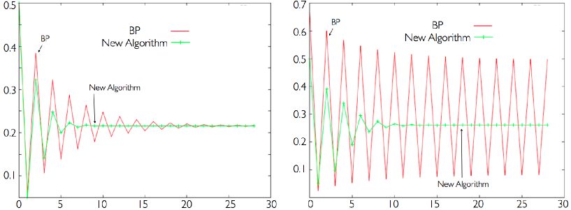
Figure 1: Comparisons of the standard BP and our new algorithm, Algorithm A, in hard-core models. In both figures, $x$-axis and $y$-axis are for the number of iterations and for the BP estimation of the marginal probability at node $(0,0)$, respectively. The left and right figures are for $\lambda=1$ and $\lambda=2$, respectively. In both cases, our algorithm converges faster than BP.

Ising Model.

The Ising model, which is named after the physicist Ernst Ising [16], is a popular mathematical model in statistical mechanics. In this model, the ‘edge’ potential functions are decided as

$$\psi_{u,v}(1,1)=\psi_{u,v}(0,0)=e^{\beta J_{u,v}}\qquad\psi_{u,v}(0,1)=\psi_{u,v}(1,0)=1,$$

where $\beta>0$ and $J_{u,v}$ are called ‘inverse temperature’ and ‘interaction’, respectively. For the ‘node’ potential functions, we choose $\psi_{v}(1)$ uniformly at random in $[1/2,2]$ independently for each $v\in V$ and set $\psi_{v}(0)=1$ deterministically.

We report the simulation results for the Ising model in Figure 2, where the left and right figures are obtained for $e^{\beta J_{u,v}}=2$ (ferromagnetic) and $e^{\beta J_{u,v}}=1/2$ (anti-ferromagnetic) for all $(u,v)$ in $E$, respectively. In both cases, we observe that the standard BP algorithm converges faster than Algorithm A. However, we note that we did not make any significant efforts to choose a better step-size in Algorithm A so that it converges faster.

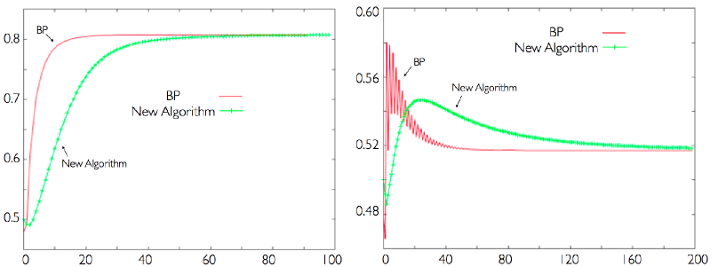
Figure 2: Comparisons of the standard BP and our new algorithm, Algorithm A, in Ising models. In both figures, $x$-axis and $y$-axis are for the number of iterations and for the BP estimation of the marginal probability at node $(0,0)$, respectively. The left and right figures are for $e^{\beta J_{u,v}}=2$ and $e^{\beta J_{u,v}}=1/2$, respectively. In both cases, our algorithm converges slower than BP.

6 Conclusion

In the last decade, exciting progress has been made on understanding computationally hard problems in computer science using a variety of methods from statistical physics. The belief propagation (BP) algorithm or its variants are among them and suggest to solve certain ‘relaxations’ of hard problems. In this paper, we address the question whether the relaxation is indeed computationally easy to solve in a strong sense. We believe that our rigorous complexity analysis of the BP-relaxation is an important step to guarantee the complexity of BP-based algorithms.

7 Acknowledgment

We are grateful to Pascal Vontobel, Devavrat Shah and anonymous reviewers for their fruitful comments on this paper. We are also grateful to Max Welling for pointing out the similarity between our algorithm and that in [25].

Appendix A Proof of Lemma 1

To simplify notation, we use $a=b\cdot e^{\pm\varepsilon}$ to mean $b\cdot e^{-\varepsilon}\leq a\leq b\cdot e^{\varepsilon}$. Now from $\left|\frac{\partial F}{\partial y_{v}}\right|\leq\varepsilon$ and $\left|\frac{\partial F}{\partial y_{u,v}}\right|\leq\varepsilon$ (i.e., the assumption $\|\nabla F(\mathbf{y})\|_{\infty}\leq\varepsilon$ in Lemma 1), we have

$$\frac{\psi_{u}(1)}{\psi_{u}(0)}\cdot\frac{\psi_{u,v}(1,0)}{\psi_{u,v}(0,0)}\cdot\frac{1-y_{v}-y_{u}+y_{u,v}}{y_{u}-y_{u,v}}\cdot\prod_{w\in\mathcal{N}(u)\setminus v}m_{w\to u}=e^{\pm\varepsilon}.$$

$$e^{\Psi^{(u,v)}}\cdot\frac{y_{u}-y_{u,v}}{1-y_{u}-y_{v}+y_{u,v}}\cdot\frac{y_{v}-y_{u,v}}{y_{u,v}}=e^{\pm\varepsilon}.$$

Using the above inequalities, the desired conclusion of Lemma 1 follows as

$$m_{u\to v} = \frac{\psi_{u,v}(0,1)}{\psi_{u,v}(0,0)}\cdot\frac{1-y_{v}-y_{u}+y_{u,v}}{1-y_{v}}\cdot\frac{y_{v}}{y_{v}-y_{u,v}}$$

$$= \frac{\psi_{u,v}(0,1)}{\psi_{u,v}(0,0)}\cdot\frac{1+\frac{y_{u,v}}{y_{v}-y_{u,v}}}{1+\frac{y_{u}-y_{u,v}}{1-y_{v}-y_{u}+y_{u,v}}}$$

$$= \frac{\psi_{u,v}(0,1)}{\psi_{u,v}(0,0)}\cdot\frac{1+e^{\pm\varepsilon}\cdot e^{\Psi^{(u,v)}}\cdot\frac{y_{u}-y_{u,v}}{1-y_{u}-y_{v}+y_{u,v}}}{1+\frac{y_{u}-y_{u,v}}{1-y_{v}-y_{u}+y_{u,v}}}$$

$$= \frac{\psi_{u,v}(0,1)}{\psi_{u,v}(0,0)}\cdot\frac{1+e^{\pm 2\varepsilon}\cdot e^{\Psi^{(u,v)}}\cdot\frac{\psi_{u}(1)}{\psi_{u}(0)}\cdot\frac{\psi_{u,v}(1,0)}{\psi_{u,v}(0,0)}\cdot\prod_{w\in\mathcal{N}(u)\setminus v}m_{w\to u}}{1+e^{\pm\varepsilon}\cdot\frac{\psi_{u}(1)}{\psi_{u}(0)}\cdot\frac{\psi_{u,v}(1,0)}{\psi_{u,v}(0,0)}\cdot\prod_{w\in\mathcal{N}(u)\setminus v}m_{w\to u}}$$

$$= e^{\pm 3\varepsilon}\cdot\frac{\psi_{u,v}(0,1)}{\psi_{u,v}(0,0)}\cdot\frac{1+e^{\Psi^{(u,v)}}\cdot\frac{\psi_{u}(1)}{\psi_{u}(0)}\cdot\frac{\psi_{u,v}(1,0)}{\psi_{u,v}(0,0)}\cdot\prod_{w\in\mathcal{N}(u)\setminus v}m_{w\to u}}{1+\frac{\psi_{u}(1)}{\psi_{u}(0)}\cdot\frac{\psi_{u,v}(1,0)}{\psi_{u,v}(0,0)}\cdot\prod_{w\in\mathcal{N}(u)\setminus v}m_{w\to u}}$$

$$= e^{\pm 3\varepsilon}\cdot f_{u\to v}\left(\prod_{w\in\mathcal{N}(u)\setminus v}m_{w\to u}\right)$$

$$= (1\pm 6\varepsilon)\cdot f_{u\to v}\left(\prod_{w\in\mathcal{N}(u)\setminus v}m_{w\to u}\right).$$

Appendix B Intuition for Lemma 1

We provide some intuition for (8) under assuming that $G$ is a tree graph. Since the BP marginal estimates $\tau_{v}(\cdot),\tau_{u,v}(\cdot)$, or equivalently the Bethe stationary points $y_{v},y_{u,v}$, are exact for tree graphs, we have that

$$\frac{1-y_{v}-y_{u}+y_{u,v}}{1-y_{v}}\cdot\frac{y_{v}}{y_{v}-y_{u,v}}~{}=~{}\frac{\Pr(x_{u}=0,x_{v}=0)}{\Pr(x_{v}=0)}\cdot\frac{\Pr(x_{v}=1)}{\Pr(x_{u}=0,x_{v}=1)}~{}=~{}\frac{\Pr(x_{u}=0~{}|~{}x_{v}=0)}{\Pr(x_{u}=0~{}|~{}x_{v}=1)}.$$

Hence, (8) is equivalent to

$${m_{u\to v}}~{}=~{}\frac{\psi_{u,v}(0,1)}{\psi_{u,v}(0,0)}\cdot\frac{\Pr(x_{u}=0~{}|~{}x_{v}=0)}{\Pr(x_{u}=0~{}|~{}x_{v}=1)}~{}=~{}\frac{\psi_{u,v}(0,1)}{\psi_{u,v}(0,0)}\cdot\frac{\Pr_{T}(x_{u}=0~{}|~{}x_{v}=0)}{\Pr_{T}(x_{u}=0~{}|~{}x_{v}=1)},$$

where $T$ be the subtree of $G$ cutting all branches attached to $v$ except for that including $u$ and $\Pr_{T}(\cdot)$ denotes the probability distribution defined by the natural induced graphical model on $T$ (using same potential functions). Furthermore, it is easy to check that BP fixed-point messages satisfy $\frac{\psi_{v}(1)}{\psi_{v}(0)}\cdot{m_{u\to v}}=\frac{\Pr_{T}(x_{v}=1)}{\Pr_{T}(x_{v}=0)}$ since $G,T$ are trees. Therefore, it follows that

$$\eqref{eq:convert}~{}~{}\Leftrightarrow {m_{u\to v}}=\frac{\psi_{u,v}(0,1)}{\psi_{u,v}(0,0)}\cdot\frac{\Pr_{T}(x_{u}=0~{}|~{}x_{v}=0)}{\Pr_{T}(x_{u}=0~{}|~{}x_{v}=1)}$$

$$\Leftrightarrow \frac{\psi_{v}(0)}{\psi_{v}(1)}\cdot\frac{\Pr_{T}(x_{v}=1)}{\Pr_{T}(x_{v}=0)}=\frac{\psi_{u,v}(0,1)}{\psi_{u,v}(0,0)}\cdot\frac{\Pr_{T}(x_{u}=0~{}|~{}x_{v}=0)}{\Pr_{T}(x_{u}=0~{}|~{}x_{v}=1)}$$

$$\Leftrightarrow \frac{\psi_{v}(0)}{\psi_{v}(1)}\cdot\frac{\psi_{u,v}(0,0)}{\psi_{u,v}(0,1)}=\frac{\Pr_{T}(x_{u}=0,x_{v}=0)}{\Pr_{T}(x_{u}=0,x_{v}=1)}.$$

In the above, the last equality can be verified easily using the fact that $v$ is a leave of tree $T$.

References

- [1] A. Bandyopadhyay and D. Gamarnik. Counting without sampling: new algorithms for enumeration problems using statistical physics. Proceedings of the Seventeenth Annual ACM-SIAM Symposium on Discrete algorithm, 890-899, 2006.
- [2] H. A. Bethe. Statistical theory of superlattices. Proc. Roy. Soc. London A, 150:552-558, 1935.
- [3] C. Berrou, A. Glavieux and P. Thitimajshima. Near shannon limit error-correcting coding and decoding: turbo codes (I). Proceeding of ICC (Geneva), 1993.
- [4] V. Chandrasekaran, M. Chertkov, D. Gamarnik, D. Shah and J. Shin. Counting independent sets using the Bethe approximation. SIAM Jouurnal on Discrete Mathematics, 25(2):1012-1034, 2011.
- [5] V. Chandrasekaran, N. Srebro and P. Harsha. Complexity of inference in graphical models, Proceedings of the Twenty-Fourth Conference Annual Conference on Uncertainty in Artificial Intelligence (UAI), AUAI Press, 70-78, 2008.
- [6] M. Chertkov and V. Y. Chernyak. Loop series for discrete statistical models on graphs. Journal of Statistical Mechanics: Theory and Experiment, P06009, 2006.
- [7] C. Daskalakis and C. Papadimitriou. Continuous local search. Proceedings of ACM-SIAM Symposium on Discrete Algorithms (SODA), 790–804, 2011.
- [8] A. Dembo and A. Montanari. Ising models on locally tree-like graphs. The Annals of Applied Probability, 20(2): 565-592, 2010.
- [9] C. Domb and M. S. Green. Phase Transitions and Critical Phenomena. Vol. 2. Academic Press. London, 1972.
- [10] D. A. Forsyth, J. Haddon and S. Ioffe. The joy of sampling. International Journal of Computer Vision, 41(1):109-134, 2001.
- [11] W. T. Freeman and E. C. Pasztor. Learning low level vision. Proceedings of International Conference of Computer Vision, 2:1182-1189, 1999.
- [12] R. G. Gallager. Low-density parity-check codes. M.I.T. Press, Cambridge, MA, 1963.
- [13] D. S. Gaunt and M. E. Fisher. Hard-sphere lattice gases. I. plane-square lattice. Journal of Chemical Physics, 43(8):2840-2863, 1965.
- [14] T. Heskes. On the uniqueness of loopy belief propagation fixed points. Neural Computation, 16(11):2379-2413, 2004.
- [15] A. T. Ihler, J. W. Fischer III and A. S. Willsky. Loopy belief propagation: convergence and effects of message errors. The Journal of Machine Learning Research, 6:905-936, 2005.
- [16] E. Ising. Beitrag zur Theorie des Ferromagnetismus. Z. Phys, 31:253-258, 1925.
- [17] S. L. Lauritzen. Graphical Models. Oxford University Press, USA, 1996.
- [18] R. J. McEliece, D. J. C. Mackay and J. F. Cheng. Turbo decoding as an instance of Pearl’s belief propagation algorithm. IEEE Journal on Selected Areas in Communication, 16(2):140-152, 1998.
- [19] K. P. Murphy, Y. Weiss and M. Jordan. Loopy belief propagation for approximate inference: an empirical study. Proceedings of Uncertainty in Artificial Intelligence, 467-475, 1999.
- [20] J. Pearl. Reverend Bayes on inference engines: A distributed hierarchical approach. Proceedings of the Second National Conference on Artificial Intelligence, AAAI Press, USA, 1982.
- [21] F. Ricci-Tersenghi and G. Semerjian. On the cavity method for decimated random constraint satisfaction problems and the analysis of belief propagation guided decimation algorithms. J. Stat. Mech., P09001, 2009
- [22] N. Ruozzi. The Bethe partition function of log-supermodular graphical models. The Neural Information Processing Systems (NIPS), 117-125, 2012.
- [23] E. B. Sudderth, M. J. Wainwright, and A. S. Willsky. Loop series and Bethe variational bounds in attractive graphical models. Advances in Neural Information Processing Systems, 20:1425–1432, 2008.
- [24] S. Tatikonda and M. Jordan. Loopy belief propagation and Gibbs measures. Uncertainty in Artificial Intelligence, 493-500, 2002.
- [25] Y. W. Teh and M. Welling. Belief optimization for binary networks: a stable alternative to loopy belief propagation. Proceedings of the Eighteenth conference on Uncertainty in artificial intelligence, 493-500, 2001.
- [26] P. O. Vontobel. Counting in graph covers: a combinatorial characterization of the bethe entropy function. Arxiv preprint arXiv:1012.0065, 2010.
- [27] M. J. Wainwright, T. Jaakkola and A. S. Willsky. Tree-based reparameterization framework for analysis of sum-product and related algorithms. IEEE Transactions on Information Theory, 45(9):1120-1146, 2003.
- [28] Y. Weiss. Correctness of local probability propagation in graphical models with loops. Neural Computation, 12(1):1-41, 2000.
- [29] J. Yedidia, W. Freeman, and Y. Weiss. Constructing free energy approximations and generalized belief propagation algorithms. IEEE Transactions on Information Theory, 51:2282-2312, 2004.
- [30] A. L. Yuille. CCCP algorithms to minimize the Bethe and Kikuchi free energies: Convergent alternatives to belief propagation. Neural Computation, 14(7):1691-1722, 2002.