Wavelets and wavelet-like transforms on the sphere
and their application to geophysical data inversion

Abstract

Many flexible parameterizations exist to represent data on the sphere. In addition to the venerable spherical harmonics, we have the Slepian basis, harmonic splines, wavelets and wavelet-like Slepian frames. In this paper we focus on the latter two: spherical wavelets developed for geophysical applications on the cubed sphere, and the Slepian “tree”, a new construction that combines a quadratic concentration measure with wavelet-like multiresolution. We discuss the basic features of these mathematical tools, and illustrate their applicability in parameterizing large-scale global geophysical (inverse) problems.

1 Introduction

This paper is about parameterization, and its role in geophysical inverse problems: the analysis and representation of volumetric properties, with a particular emphasis on the three-dimensional ball and its surface, the two-dimensional sphere. This is not the sole purview of geophysics (e.g. geodesy, geodynamics, seismology): there is a large literature on the subject in virtually every area of scientific inquiry (e.g. medical imaging, astronomy, cosmology, computer graphics, image processing, …). For this reason we limit ourselves here to a few technical aspects, some of which have been published before (refs 1, 2) but are illustrated with different examples.

We begin with a new class of spherical wavelet basis on the ball designed for the analysis of geophysical models and for the tomographic inversion of global seismic data[3, 4, 1]. Its multiresolution character allows for modeling with an effective spatial resolution that varies with position within the Earth. We introduce two types of discrete wavelet transforms in the angular dimension of the “cubed sphere”, a well-known Cartesian-to-spherical mapping[5, 6]. These are applied to analyze the information of terrestrial topography data and in seismic wavespeed models of the Earth’s mantle across scale space. The localization and sparsity properties of the wavelet bases allow finding a sparse solution to inverse problems by iterative minimization of a combination of the $\ell_{2}$ norm of the data residuals and the $\ell_{1}$ norm of the model wavelet coefficients. These have now been validated in realistic synthetic experiments to likely yield important gains in the inversion of seismic data for global seismic tomography, the procedure by which seismic waveforms are being used to image the three-dimensional distribution of elastic (compressional or P and shear or S) wave speeds ($V_{P}$ and $V_{S}$) inside the Earth.

A second class of transforms is inspired by the type known as Slepian functions. These we understand to be families of orthogonal functions that are all defined on a common, e.g. geographical, domain, where they are either optimally quadratically concentrated or within which they are exactly limited, and which at the same time are exactly confined within a certain bandwidth, or maximally concentrated therein. Originally developed for the study of time series by Slepian, Landau and Pollak[7, 8] in the 1960s, they have now been fully extended to the multidimensional Cartesian plane[9, 10] and the surface of the sphere[11, 12, 13], where most of the geophysical applications lie. We have reported on some aspects of spherical Slepian functions and their role in the analysis and representation of geophysical data in previous papers in this series[14, 15]. In this contribution we announce a hybrid construction that blends desirable aspects and properties of Slepian functions with ideas from wavelet and frame theory. We summarize the main ideas contained in Chapter 7, Multiscale Dictionaries of Slepian Functions on the Sphere, of the Ph. D. thesis by Eugene Brevdo[2], deferring a full publication to a later date.

2 Wavelets on the Cubed Sphere

The use of wavelets is still no matter of routine in global geophysics, beyond applications in one and two Cartesian dimensions. This despite there being a wealth of available constructions on the sphere[16, 17, 18, 19, 20, 21, 22, 23, 24, 25, 26, 27, 28]. However, the cited studies are mostly concerned with surfaces, not volumes, and many of them require custom design and special algorithms. For the application to global seismic tomography that we envisage, we take advantage of the ease and flexibility of existing Cartesian constructions by implementing standard algorithms on a spherical-to-Cartesian map proposed by Ronchi et al. (1996), a grid that has long since proven its utility in the geosciences and beyond.

As in ref. 5, we define a coordinate 4-tuple $(\xi,\eta,r,\kappa)$ for each of the $\kappa=1\rightarrow 6$ “chunks” comprising this “cubed sphere” at radius $r$. In ref. 1 we list explicit formulas for the forward and inverse mapping of cubed-sphere to Cartesian coordinates. Here we suffice to say that a “master” surface chunk defined by the $2\times 2^{N}$ linearly spaced coordinate pairs $-\pi/4\leq(\xi,\eta)\leq\pi/4$ maps, in a general sense, to the Cartesian coordinate vector

$$[\,x,y,z\,]=[1\quad\tan\eta\quad-\tan\xi\,]\,(1+\tan^{2}\xi+\tan^{2}\eta)^{-1/2},$$ (1)

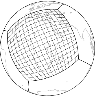
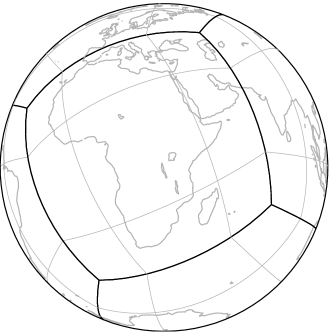
Figure 1: Aerial view showing our adaptations of the cubed sphere of ref. 5. Of the front-facing four of the in total six “chunks”, one is gridded to reveal its $2^{2N}$ surface elements ($N=4$). The thick black lines identify the boundaries of the six “chunks”. The thin gray lines correspond to the boundaries of the overlapping “superchunks” as discussed in the text.

which is rotated to occupy a total of six non-overlapping patches tiling the sphere, after which the entire construction is rotated over a standard set of Euler angles $\alpha=0.0339$, $\beta=1.1705$, and $\gamma=1.1909$. This results in the configuration shown in Figure 1 (left).

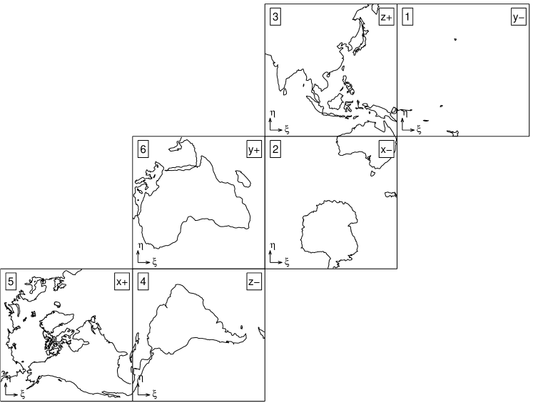
Figure 2: Geometry, nomenclature, and numbering of the six faces of our cubed sphere in a two-dimensional view.

Alternatively, for reasons that will be made clear, we start from the coordinates $-3\pi/8\leq(\xi,\eta)\leq 3\pi/8$ and apply the same rotations, thereby producing six overlapping “superchunks”, as in Figure 1 (right). Throughout this paper we will quote $N$ as the angular resolution level of our cubed sphere, which implies that it has $6\times 2^{2N}$ such elements, with typical seismic tomography grids having $N=7$. The Euler angles used in our construction were chosen for geographical convenience, as can be seen from the continental outlines in Figure 2.

On these two grids we apply standard Cartesian transforms, e.g. orthogonal[29] and bi-orthogonal[30] ones, whereby for the case of the non-overlapping “chunks” construction we accommodate the presence of the “seams’ by switching to special boundary filters at each of the edges, and applying preconditioners to the data prior to transformation in order to guarantee the usual polynomial cancellation throughout the closed rectangular interval, as is well established[31]. With this choice of bases, sparsity in the representation of many data types is to be generally expected[32].

In Figure 3 we explore coefficient statistics and the effects of thresholding on the reconstruction errors for a model of terrestrial topography. We focus on the fifth, or “North-American” chunk of our cubed sphere, and use the orthogonal D2 (Haar), D4 and D6 wavelet bases[29] on the interval, with preconditioning[31]. The top row uses the common conventions in plotting the wavelet and scaling coefficients in each of the bases after (hard) thresholding[32] such that only the coefficients larger than their value at the 85^th percentile level survive. The coefficients that have now effectively been zeroed out are left white in these top three panels. The middle series of panels of Figure 3 plots the spatial reconstruction after thresholding at this level; the root mean squared (rms) errors of these reconstructions are quoted as a percentage of the original root mean squared signal strengths. The thresholded wavelet transforms allow us to discard, as in these examples, 85% of the numbers required to make a map of North American topography in the cubed-sphere pixel basis: the percentage error committed is only 6.3%, 5.2% and 9.2% according to this energy criterion in the D2, D4 and D6 bases, respectively. From the map views it is clear that despite the relatively small error, the D2 basis leads to unsightly block artifacts in the reconstruction, which are largely avoided in the smoother and more oscillatory D4 and D6 bases. A view of the coefficient statistics is presented in the lowermost three panels of Figure 3. The coefficients are roughly log-normally distributed, which helps explain the success of the thresholded reconstruction approach. We conclude that the D4 basis is a good candidate for geophysical data representation.

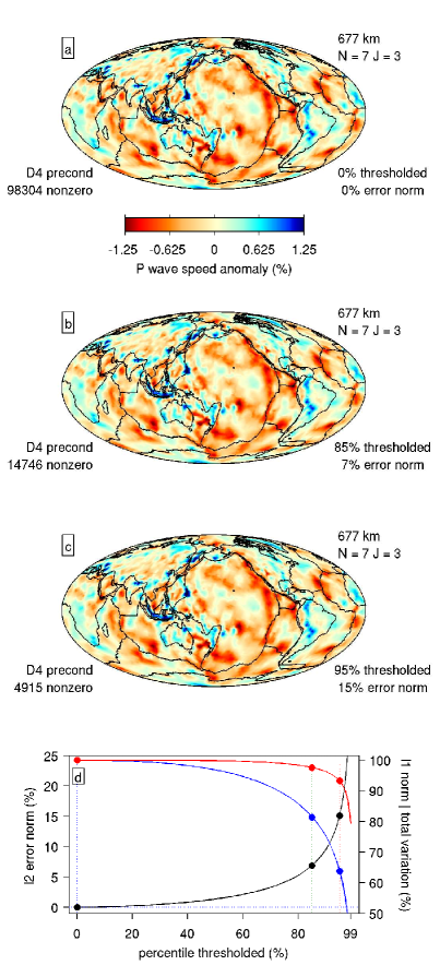
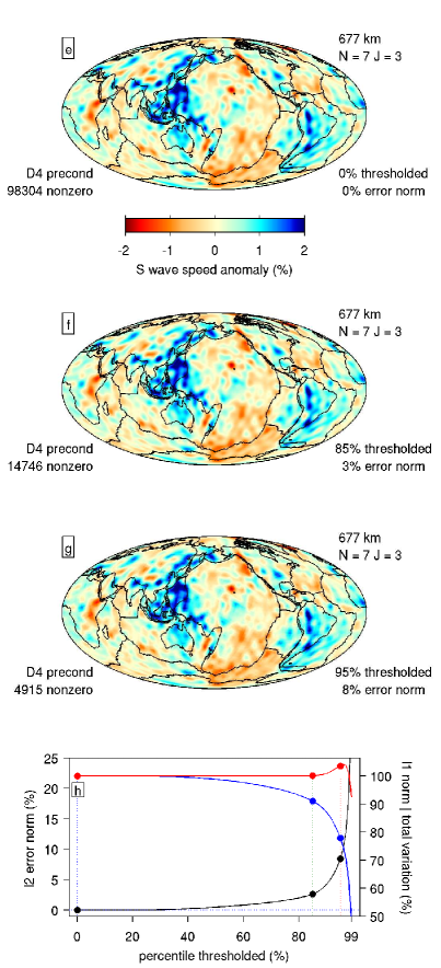
Figure 4: Sparsity and reconstruction stability of two global seismic wavespeed models under incremental hard thresholding of their wavelet and scaling coefficients using the preconditioned edge-cognizant D4 wavelet basis[29, 31] in the angular coordinates of the cubed sphere, as developed in this paper. (a–d) Results for the compressional wave speed seismic model of ref. 43 and (e–h) for the shear wave speed seismic model of ref. 44, at the same depth of 677 km below the surface of the Earth, for cubed spheres with $6\times 2^{2N}$ elements ($N=7$), and to a $2^{J}$ dyadic subdivision ($J=3$). As a function of the percentage of the coefficients that are being thresholded, and relatively to the original unthresholded values, the bottom panels quote the spatial $\ell_{2}$ norms of the reconstruction error (in black), the total variation norms of the reconstructed images in the space domain (in red), and the $\ell_{1}$ norms of the coefficients that remain (in blue). The reconstructions remain faithful to the originals even at elevated levels of thresholding.

For applications in seismology we now illustrate the performance of the cubed-sphere wavelet basis in compressing seismological Earth models such as the one by Montelli et al. (2006) of compressional (P) wavespeed heterogeneity and another by Ritsema et al. (2010) of shear (S) wavespeed perturbations. At a depth of about 670 km, Figs 4a and 4e show the wavespeed anomalies from the average at that depth. The wavelet transform in the D4 basis (with special boundary filters and after preconditioning, and up until scale $J=3$) was thresholded and the results re-expanded to the spatial grid, identically as we did for the topography in Figure 3. The results for specific values of the thresholding (quoted as the percentile of the original wavelet coefficients) are shown in Figs 4b and 4f for the 85^th, and Figs 4c and 4g for the 95^th, respectively. At each level of thresholding the number of nonzero wavelet/scaling expansion coefficients is quoted: at 0% thresholding this number is identical to the number of pixels in the surficial cubed sphere being plotted.

The reconstruction error can be visually assessed from the pictures; it is also quoted next to each panel as the percentage of the root mean squared error between the original and the reconstruction, normalized by the root mean squared value of the original in the original pixel representation, in percent. Specifically, we calculate and quote the ratio of $\ell_{2}$ norms in the pixel-basis model vector ${\mathbf{m}}$,

$$100\times\left.\left\|{\mathbf{m}}-{{S}}\left\{{\mathcal{T}}\!\left[{{A}}({\mathbf{m}})\right]\right\}\right\|_{2}\right/\left\|{\mathbf{m}}\right\|_{2},$$ (2)

which, in the lower-right annotations is called the “% error norm”. We write ${{A}}$ for any of the wavelet (analysis) transforms that can be used and ${{S}}$ (synthesis) for their inverses, and ${\mathcal{T}}$ for the hard thresholding of the wavelet and scaling coefficients. In Figs 4e and 4j, the misfit quantity (2) is represented as a black line relevant to the left ordinate labeled “$\ell_{2}$ error norm”, which shows its behavior at 1% intervals of thresholding; the filled black circles correspond to the special cases shown in the map view. Only after about 80% of the coefficients have been thresholded does the error rise above single-digit percentage levels, but after that, the degradation is swift and inexorable. The blue curves in Figs 4e and 4j show another measure relevant in this context, namely the ratio of the $\ell_{1}$ norms of the thresholded wavelet coefficients compared to the original ones, in percent, or

$$100\times\left.\left\|{\mathcal{T}}\!\left[{{A}}({\mathbf{m}})\right]\right\|_{1}\right/\left\|{{A}}({\mathbf{m}})\right\|_{1}.$$ (3)

The $\ell_{2}$ ratios (2) in the black curves (and the left ordinate) evolve roughly symmetrically to the $\ell_{1}$ ratios (3) in the blue curves (and the right ordinate), though evidently their range is different. The third measure that is being plotted as the red curve is the “total variation” norm ratio, in percent, namely

$$100\times\left.\left\|\mbox{\boldmath$\nabla$}{{S}}\left\{{\mathcal{T}}\!\left[{{A}}({\mathbf{m}})\right]\right\}\right\|_{1}\right/\left\|\mbox{\boldmath$\nabla$}{\mathbf{m}}\right\|_{1},$$ (4)

whereby $\left\|\mbox{\boldmath$\nabla$}{\mathbf{m}}\right\|_{1}$ is the sum over all voxels of the length of the local gradient of ${\mathbf{m}}$. By this measure, which is popular in image restoration applications[33, 34, 35], the quality of the reconstruction stays very high even at very elevated levels of thresholding; we note that its behavior is not monotonic and may exceed 100%.

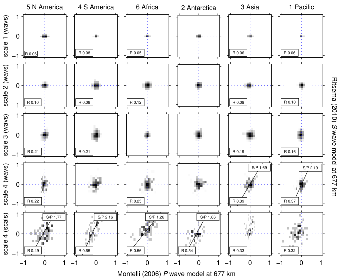
Figure 5: Joint properties of seismic mantle structure in the Montelli (2006) P-wave and Ritsema (2010) S-wave speed models, at 677 km depth in the Earth. Every row corresponds to a different scale in the D4 wavelet decomposition of the models. Each panel shows the logarithmic density of observations. Black shading corresponds to the maximum density in each panel; all patches that account for less than 1% of the observations are rendered white. Using total least squares a regression line was fit to all sets with correlation coefficients exceeding 0.35. The slope of the line, a measure of the $\delta\ln V_{S}/\delta\ln V_{P}$ ratio appears in the top right corners. Significant correlation coefficients are quoted in the bottom left.

Finally, the new wavelet construction can be used to study the joint properties of the wavelet coefficients of seismic wavespeed models, as we illustrate in Figure 5. There, we report the correlation between wavelet coefficients in the Montelli and Ritsema models as a function of scale and approximate geographical position (see again Figure 2 for the numbering scheme of the cubed-sphere chunk). A rendering of the two-dimensional density of the data is accompanied by the value of their correlation coefficient (lower left labels) where this is deemed significant at the 95% level, and the slope of the total-least-squares based fit in this space (upper right labels), which is only quoted when the correlation coefficients exceeded 0.35. This should provide an estimate of the logarithmic ratio of shear-wave to compressional-wave speed perturbations, $\delta\ln V_{S}/\delta\ln V_{P}$, an important discriminant in the interpretation of the (thermal or chemical) cause of seismic velocity anomalies [36]. The variation of this ratio as a function of scale and chunk position yields information that will be of use for geochemical and geodynamical studies, and the orthogonality of the wavelet basis in scale and physical space removes some of the arbitrariness in the calculation. Ritsema’s model does not have much structure at the smallest scales. From scale 3 onward a positively correlated pattern begins to emerge, though even at this particular scale, the correlation coefficients remain below the relatively stringent 0.35 level. Wavelets and scaling coefficients are well correlated at the largest scale 4 considered, with several of the correlation coefficients exceeding our threshold. This information is useful to geophysicists[37, 38, 39, 36], especially given our new-found ability to study the regional variation of such ratios, taking into account their dependence on scale length.

Simons et al. (2011) detail the reasoning behind the construction of the “superchunk” cubed sphere shown in Figure 1 (right). In a nutshell, the cubed-sphere bases are to be used not simply for the representation and analysis of seismic models, but also to parameterize the inversion of primary data for such models. Since the edge-cognizant transforms are not norm-preserving, the thresholding steps involved in using common algorithms such as (F)ISTA[3, 40, 4], if unmodified, lead to artifacts in the solution which are largely avoided by building the wavelet transforms in the superchunk domain and ignoring the edges altogether[1].

3 The Spherical Slepian Tree Transform

Geophysical and cosmological signals are constrained by the physical processes that generate them and conditioned by the sensors that observe them. On the real line and in the plane, both physical and sampling constraints lead to assumptions of a bandlimit: that a signal contains no energy outside some supporting region in the frequency domain. Bandlimited signals on the sphere are zero save for the low-frequency spherical-harmonic components. Spherical harmonics are not orthogonal on arbitrary portions of the sphere, yet for the study of geophysical processes we may not have access to nor interest in signal originating from outside a specific geographic region of interest. By construction, Slepian functions satisfy the dual constraints of bandlimitation and spatial concentration by optimization of an energy criterion that concentrates as much energy as possible into the region of interest for a given bandlimit[13]. With Slepian function bases, however, it is “all or nothing”: given a certain bandwidth and a spatial region of interest, the functions (variably) fill the entire bandwidth range and ultimately the entire spatial target. The wavelet constructions that we introduced in Section 2, on the other hand, were compactly supported and had multiresolution properties which the Slepian basis does not possess.

Here we develop an algorithm for the construction of Slepianesque dictionary elements that are bandlimited, localized, and multiscale. It is based on a subdivision scheme that constructs a binary tree from subdivisions of the region of interest. Such a dictionary has many nice properties: it closely overlaps with the most concentrated Slepian functions on the region of interest, and most element pairs have low coherence. Therefore, they, too, should be eminently suitable to solve ill-posed inverse problems in geophysics and cosmology. Though the new dictionary is no longer composed of purely orthogonal elements like the Slepian basis, it can also be combined with modern inversion techniques that promote sparsity in the solution. Thereby they provide significantly lower residual error after reconstruction when compared to “classically optimal” Slepian inversion techniques[41].

3.1 A Multiscale Dictionary of Slepian Functions

We now turn our focus to numerically constructing a dictionary ${{\mathcal{D}}}$ of functions that can be used to approximate bandlimited signals on the sphere and allows for the reconstruction of signals from their point samples. Let ${{\mathcal{R}}}\subset S^{2}$ be a simply connected subset of the sphere. With $L$ the bandwidth, the dictionary ${{\mathcal{D}}}$ will be composed of functions bandlimited to spherical harmonic degrees $0\leq l\leq L$. The construction is based on a binary tree. The node capacity, $n$, is a positive integer. Each node of the tree corresponds to the first $n$ Slepian functions with bandlimit $L$ and concentrated on a subset ${{\mathcal{R}}}^{\prime}\subset{{\mathcal{R}}}$. The top tree node is for the entire region ${{\mathcal{R}}}$, and each node’s children correspond to a division of ${{\mathcal{R}}}^{\prime}$ into two roughly equally sized subregions. As the child nodes will be concentrated in disjoint subsets of ${{\mathcal{R}}}^{\prime}$, all of their corresponding functions and children are effectively incoherent. We now fix a height $H$ of the tree: the number of times to subdivide ${{\mathcal{R}}}$. The height is determined as the maximum number of binary subdivisions of ${{\mathcal{R}}}$ that can have $n$ well concentrated functions. That is, we find the minimum integer $H$ such that $n\geq N_{2^{-H}\left|{{\mathcal{R}}}\right|,L}$, with $N$ the Shannon number[13], which has the solution

$$H=\left\lceil\log_{2}\left(\frac{\left|{{\mathcal{R}}}\right|}{4\pi}\frac{(L+1)^{2}}{n}\right)\right\rceil.$$

A complete binary tree with height $H$ has $2^{H+1}-1$ nodes, so from now on we will denote the dictionary

$${{\mathcal{D}}}_{{{\mathcal{R}}},L,n}=\big{\{}d^{(1,1)},d^{(1,2)},\cdots,d^{(1,n)},\cdots,d^{\left(2^{H+1}-1,1\right)},\cdots,d^{\left(2^{H+1}-1,n\right)}\big{\}}$$

as the set of $\left|{{\mathcal{D}}}_{{{\mathcal{R}}},L,n}\right|=n\,(2^{H+1}-1)$ functions thus constructed on region ${{\mathcal{R}}}$ with bandlimit $L$ and node capacity $n$. Figure 6 shows the tree diagram of the subdivision scheme. We use the standard enumeration of nodes wherein node $(j,\cdot)$ is subdivided into child nodes $(2j,\cdot)$ and $(2j+1,\cdot)$, and at a level $0\leq h\leq H$, the nodes are indexed from $2^{h}\leq j\leq 2^{h+1}-1$. More specifically, for ${j=1,2,\ldots}$, we have ${{{\mathcal{R}}}^{(j)}={{\mathcal{R}}}^{(2j)}\cup{{\mathcal{R}}}^{(2j+1)}}$. Furthermore, letting $g^{{{\mathcal{R}}}^{\prime}}_{\alpha}$ be the $\alpha^{\mathrm{th}}$ Slepian function on ${{\mathcal{R}}}^{\prime}$ (the solution to the classical Slepian concentration criterion eq. 4.1 in ref. 13, with concentration region ${{\mathcal{R}}}^{\prime}$), we have that

$$d^{(j,\alpha)}=g^{{{\mathcal{R}}}^{(j)}}_{\alpha}.$$

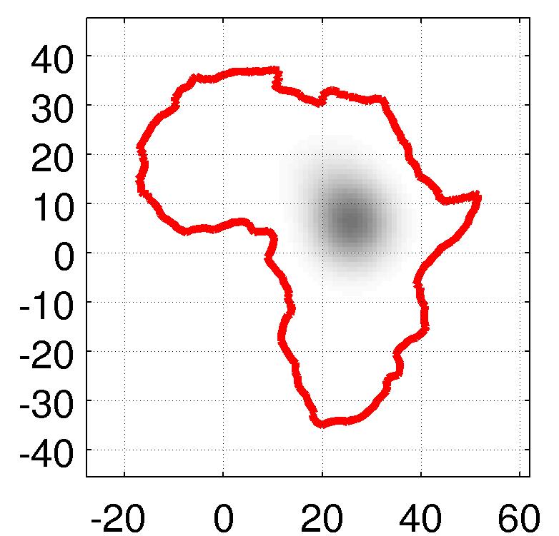
(a) $d^{(1,1)}$

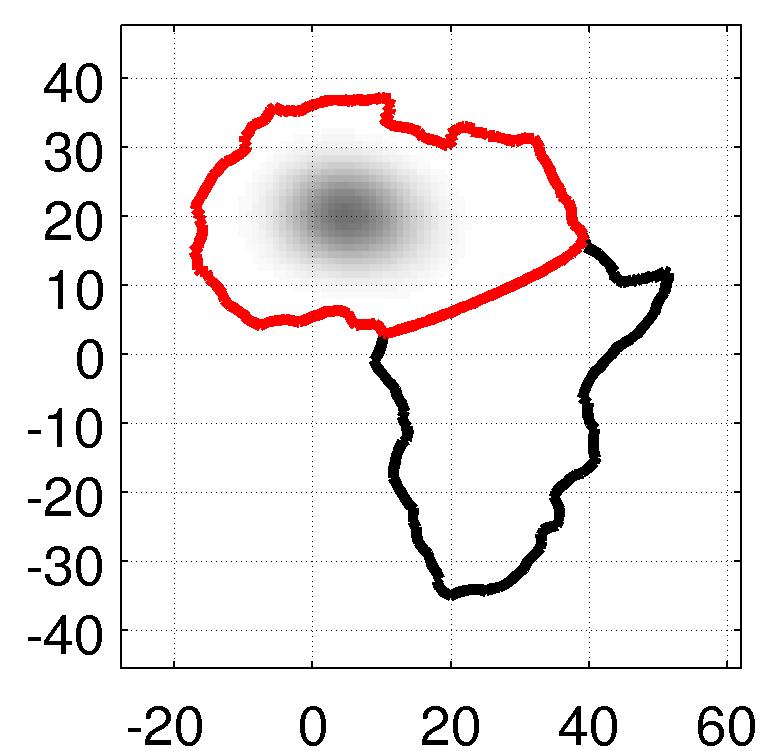
(b) $d^{(2,1)}$

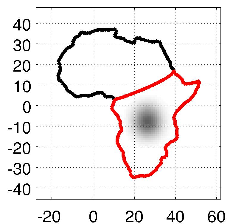
(c) $d^{(3,1)}$

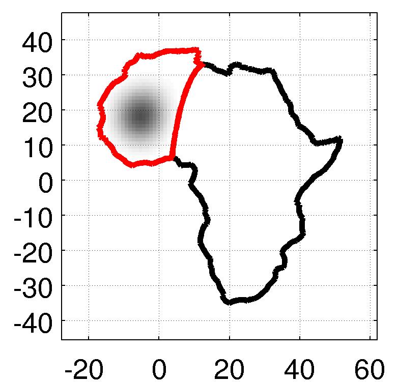
(d) $d^{(4,1)}$

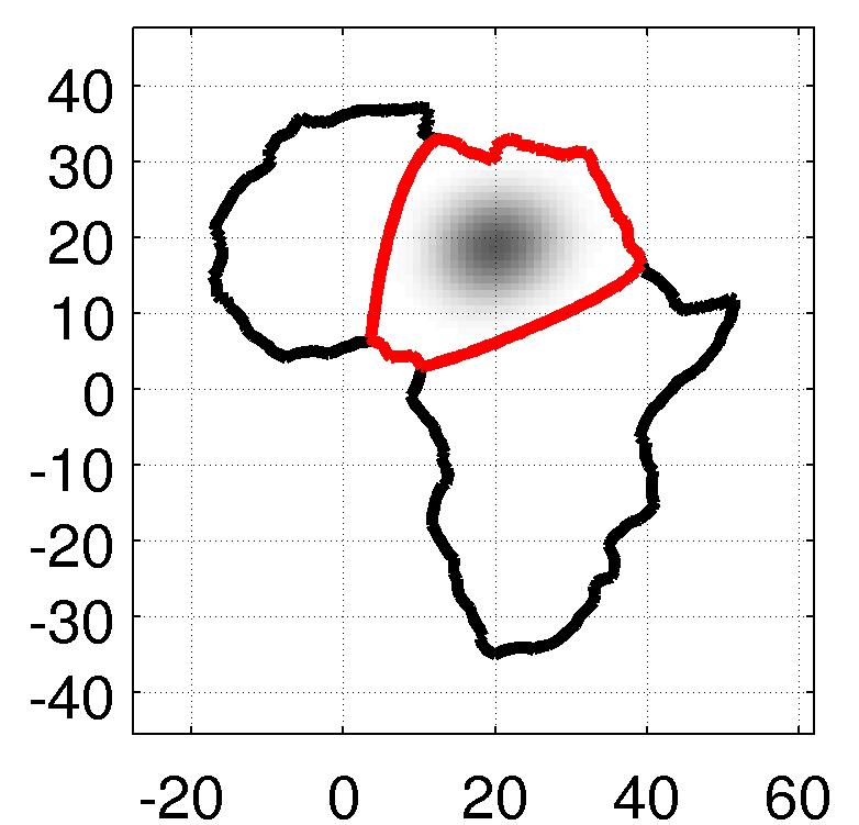
(e) $d^{(5,1)}$

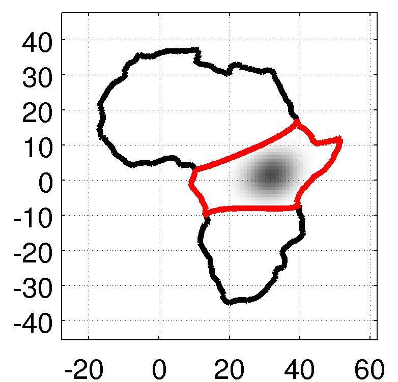
(f) $d^{(6,1)}$

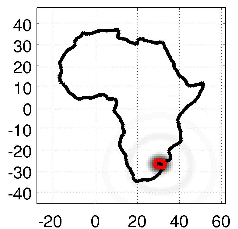
(g) $d^{(250,1)}$

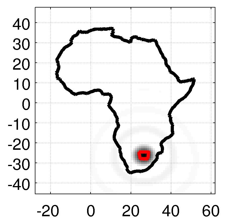
(h) $d^{(251,1)}$

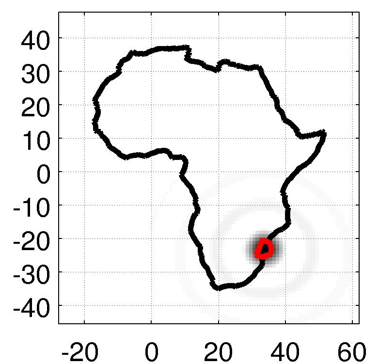
(i) $d^{(252,1)}$

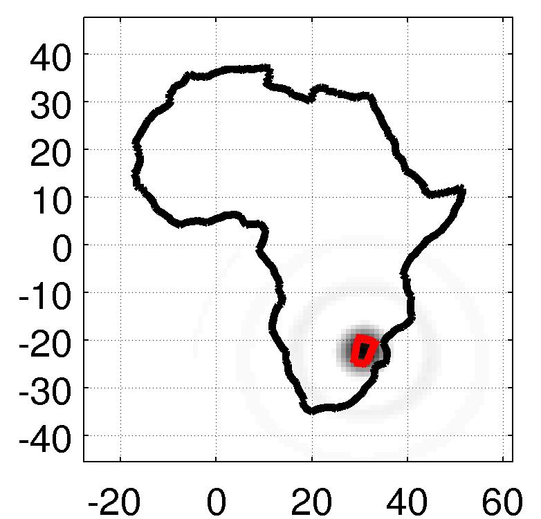
(j) $d^{(253,1)}$

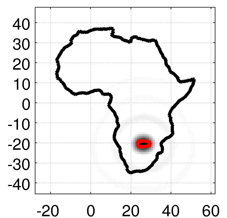
(k) $d^{(254,1)}$

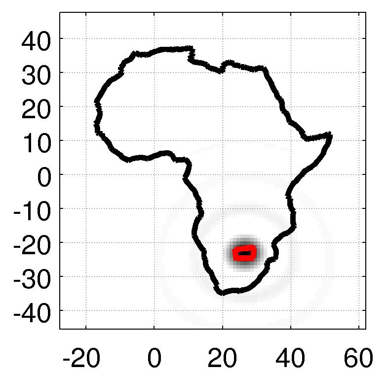
(l) $d^{(255,1)}$

Figure 7: Slepian tree dictionary ${{\mathcal{D}}}_{\textrm{\small Africa},36,1}$ of size $\left|{{\mathcal{D}}}\right|=255$ showing the functions $d^{(1,1)}$ through $d^{(6,1)}$ and $d^{(250,1)}$ through $d^{(255,1)}$. The x-axis is longitude, the y-axis is colatitude. Regions of concentration $\big{\{}{{\mathcal{R}}}^{(i)}\big{\}}$ are outlined.

Figure 7 shows an example of the construction when ${{\mathcal{R}}}$ is the African continent. Note how, for example, $d^{(4,1)}$ and $d^{(5,1)}$ are the first Slepian functions associated with the subdivided domains of ${{\mathcal{R}}}^{(2)}$.

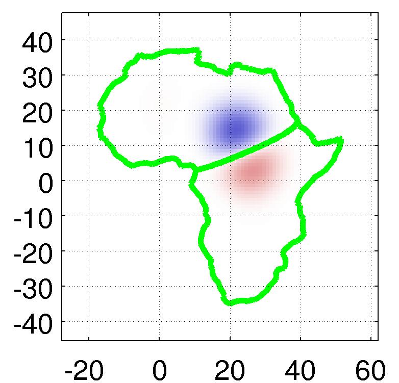
(a) $d^{(1,2)}$

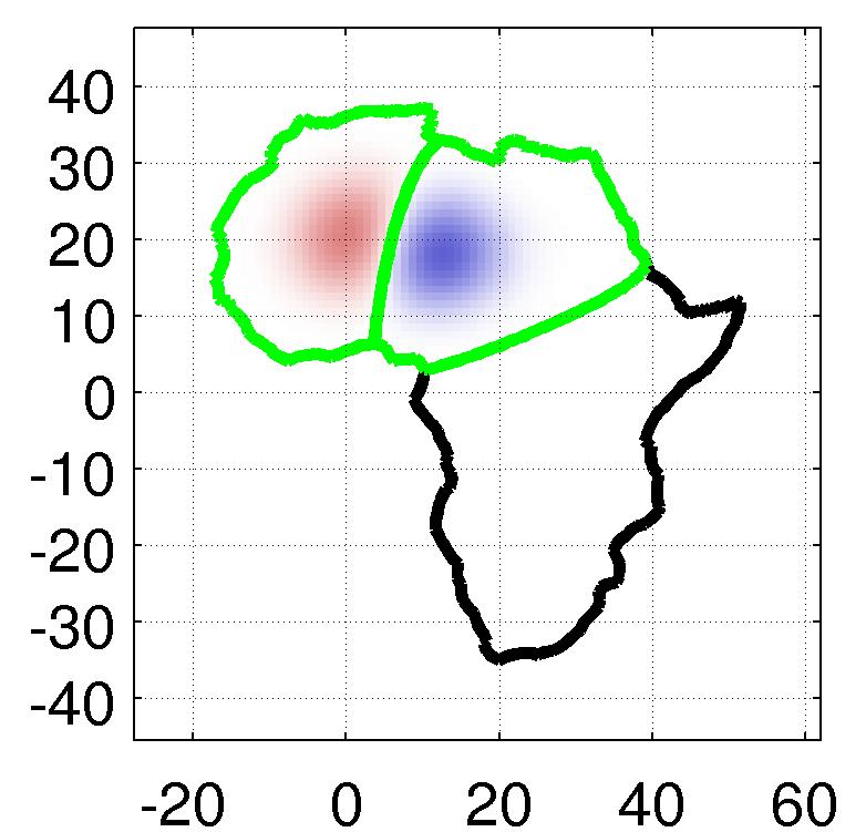
(b) $d^{(2,2)}$

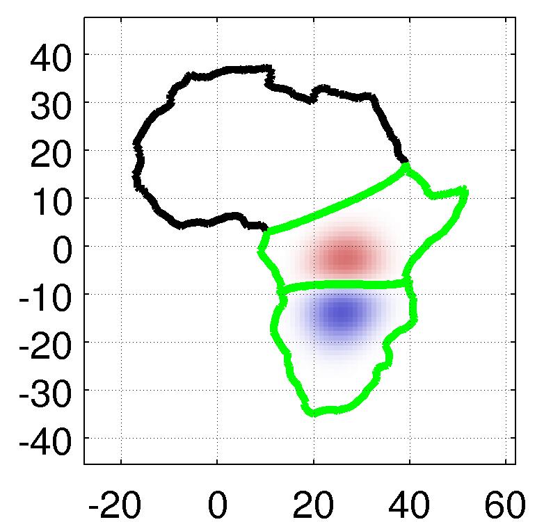
(c) $d^{(3,2)}$

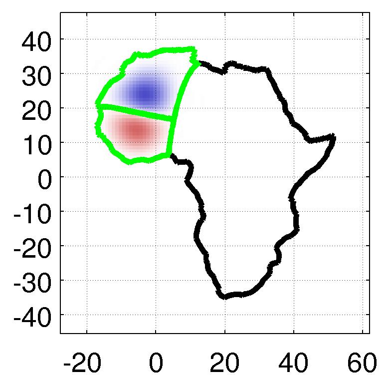
(d) $d^{(4,2)}$

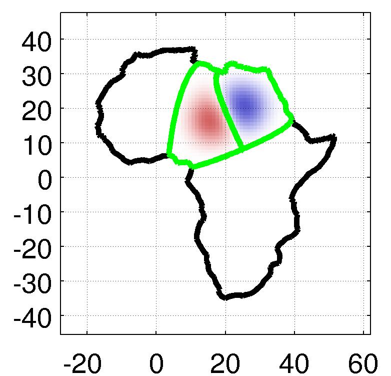
(e) $d^{(5,2)}$

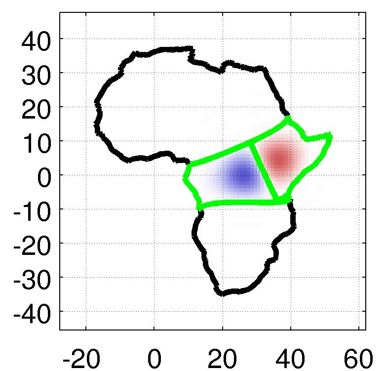
(f) $d^{(6,2)}$

Figure 8: Second ($\alpha=2$) Slepian functions associated with the regions in Figure 7a–f. Regions of concentration, and the dividing contour (the zero-level set), are drawn in green. Blue and red represent the sign of the Slepian function values.

To complete the top-down construction, it remains to decide how to subdivide a region ${{\mathcal{R}}}^{\prime}$ into equally sized subregions. For roughly circular connected domains, the first Slepian function has no sign changes, and the second Slepian function has a single zero-level curve that subdivides the region into approximately equal areas; when ${{\mathcal{R}}}^{\prime}$ is a spherical cap, the subdivision is exact [13]. We thus subdivide a region ${{\mathcal{R}}}^{\prime}$ into the two nodal domains associated with the second Slepian function on that domain; see Figure 8 for a visualization of the subdivision scheme as applied to the African continent.

3.2 Concentration, Range, and Incoherence

The utility of the tree construction presented above depends on its ability to represent bandlimited functions in a region ${{\mathcal{R}}}$, and its efficacy at reconstructing functions from point samples in ${{\mathcal{R}}}$. These properties, in turn, reduce to questions of concentration, range, and incoherence. First, dictionary ${{\mathcal{D}}}$ is concentrated in ${{\mathcal{R}}}$ if its functions are concentrated in ${{\mathcal{R}}}$. Second, the range of dictionary ${{\mathcal{D}}}$ is the subspace spanned by its elements. Ideally, the basis formed by the first few Slepian functions on ${{\mathcal{R}}}$ is a subspace of the range of ${{\mathcal{D}}}$. Third, when ${{\mathcal{D}}}$ is incoherent, pairwise inner products of its elements have low amplitude: pairs of functions are approximately orthogonal. This, in turn, is a useful property when using ${{\mathcal{D}}}$ to estimate signals from point samples.

Unlike the concentration eigenvalues corresponding to the Slepian functions on ${{\mathcal{R}}}$, not all of the eigenvalues of the elements of ${{\mathcal{D}}}_{{{\mathcal{R}}}}$ reflect their concentration within this top-level (parent) region. We thus define the modified concentration value

$$\nu^{(j,\alpha)}=\int_{{{\mathcal{R}}}}\left[d^{(j,\alpha)}(x)\right]^{2}d\mu(x).$$ (5)

Recalling that $\left\|d^{(j,\alpha)}\right\|_{2}=1$, the value $\nu$ is simply the percentage of energy of the $(j,\alpha)^{\textrm{th}}$ element that is concentrated in ${{\mathcal{R}}}$. This value is always larger than the element’s eigenvalue, which relates its fractional energy within the smaller subset ${{\mathcal{R}}}^{(j)}$.

The size of dictionary ${{\mathcal{D}}}_{{{\mathcal{R}}},L,n}$ is generally larger than the Shannon number $N_{\left|{{\mathcal{R}}}\right|,L}=(L+1)^{2}/\left|{{\mathcal{R}}}\right|/4/\pi$ for any node capacity $n$, and as a result it cannot form a proper basis: it has too many functions. Ideally, then, we require that elements of the dictionary span the space of the first $N_{\left|{{\mathcal{R}}}\right|,L}$ Slepian functions. One possible answer to the question of the range of ${{\mathcal{D}}}$ is given by studying the angle between the subspaces [42] spanned by elements of ${{\mathcal{D}}}$ and the first $\alpha$ functions of the Slepian basis, for ${\alpha=1,2,\ldots}$. The angle between two subspaces $A$ and $B$, possibly with different dimensions, is given by the formula

$$\angle(A,B)=\min\left(\sup_{x\in A}\angle(x,B),\sup_{y\in B}\angle(y,A)\right),\quad\mbox{where}\\ \angle(x,B)=\inf_{y\in B}\angle(x,y)=\cos^{-1}\frac{\left\|P_{B}x\right\|}{\left\|x\right\|}.$$ (6)

Here, $P_{B}$ is the orthogonal projection onto space $B$ and all of the norms are with respect to the given subspace. The angle $\angle(A,B)$ is symmetric, non-negative, and zero iff $A\subset B$ or $B\subset A$; furthermore it is invariant under unitary transforms applied to both on $A$ and $B$, and admits a triangle inequality. It is thus a good indicator of distance between two subspaces; furthermore, it can be calculated accurately given two matrices whose columns span $A$ and $B$. We can therefore identify the matrices $A$ and $B$ with the subspaces spanned by their columns.

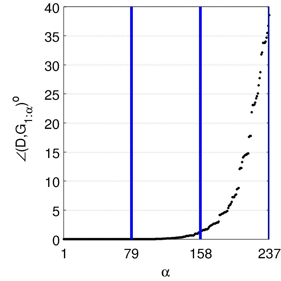
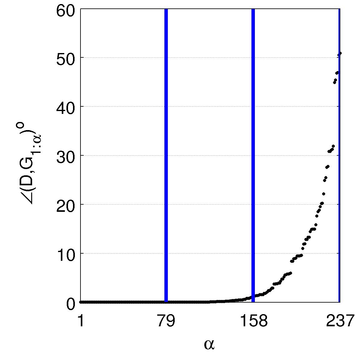
Figure 9: Angles (in degrees) between the spaces spanned by $\big{(}\widehat{G}_{\left|{{\mathcal{R}}}\right|,36}\big{)}_{1:\alpha}$ and the dictionary matrices $\widehat{D}_{{{\mathcal{R}}},36,1}$ (left) and $\widehat{D}_{{{\mathcal{R}}},36,2}$ (right), ${{\mathcal{R}}}=\textrm{\small Africa}$, $\alpha=1,\ldots,3N_{\left|{{\mathcal{R}}}\right|,L}$. Thick lines correspond to integer multiples of the Shannon number ${N_{\textrm{\small Africa},36}\approx 79}$.

Let $\big{(}\widehat{G}_{{{\mathcal{R}}},L}\big{)}_{1:\alpha}$ denote the matrix containing the first $\alpha$ column vectors which are the spherical harmonic expansion coefficients of the traditional Slepian functions for a given region ${{\mathcal{R}}}$ and a bandwidth $L$. Let $\widehat{D}$ denote the $(L+1)^{2}{\times}\left|{{\mathcal{D}}}_{{{\mathcal{R}}},L,n}\right|$ matrix containing the spherical harmonic representations of the elements of the dictionary ${{\mathcal{D}}}_{{{\mathcal{R}}},L,n}$. Figure 9 shows $\angle(\widehat{G}_{1:\alpha},\widehat{D})$ for ${{{\mathcal{R}}}=\textrm{\small Africa}}$ with ${L=36}$. The Shannon number is ${N_{\textrm{\small Africa},36}\approx 79}$. It is clear that while the dictionaries ${{\mathcal{D}}}_{\textrm{\small Africa},36,1}$ and ${{\mathcal{D}}}_{\textrm{\small Africa},36,2}$ do not strictly span the space of functions bandlimited to $L=36$ and optimally concentrated in Africa, they are a close approximation: the column span of $\big{(}\widehat{G}_{\textrm{\small Africa},36}\big{)}_{1:\alpha}$ is nearly linearly dependent with the spans of $\widehat{D}_{\textrm{\small Africa},36,1}$ and $\widehat{D}_{\textrm{\small Africa},36,2}$, for $\alpha$ significantly larger than $N_{\textrm{\small Africa},36}$.

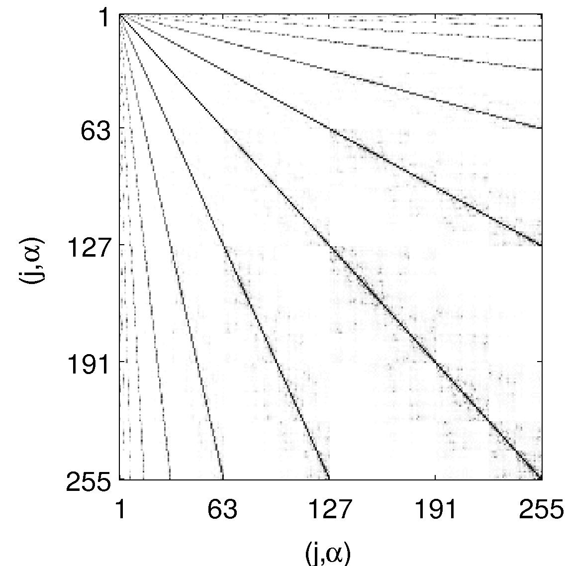
(a) ${{\mathcal{D}}}_{\textrm{\small Africa},36,1}$

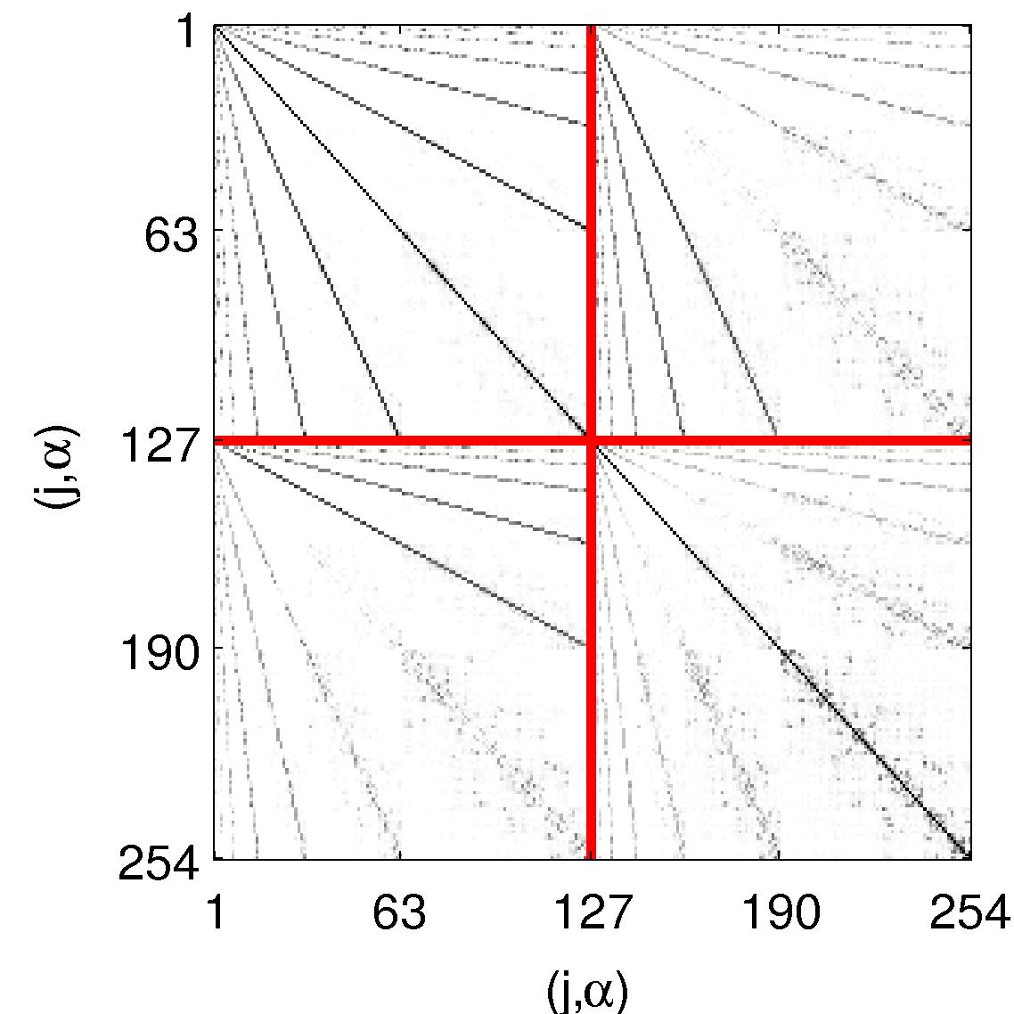
(b) ${{\mathcal{D}}}_{\textrm{\small Africa},36,2}$

Figure 10: Magnitudes of pairwise inner products of dictionaries (a) ${{\mathcal{D}}}_{\textrm{\small Africa},36,1}$ and (b) ${{\mathcal{D}}}_{\textrm{\small Africa},36,2}$. In (b), thick lines separate inner products between the 127 elements with $\alpha=1$ (top left) and $\alpha=2$ (bottom right), and their cross products. Values are between 0 (white) and 1 (black).

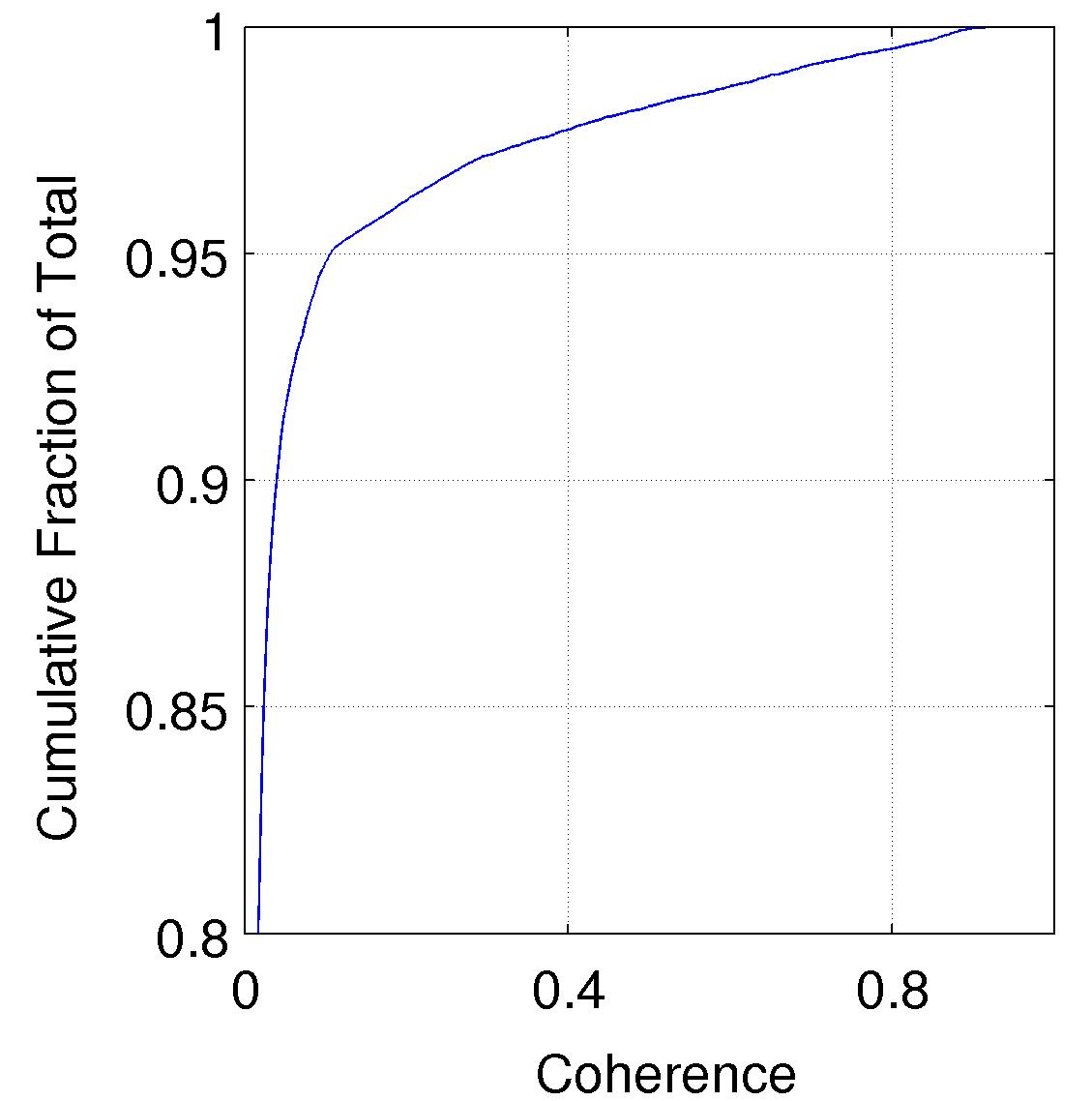
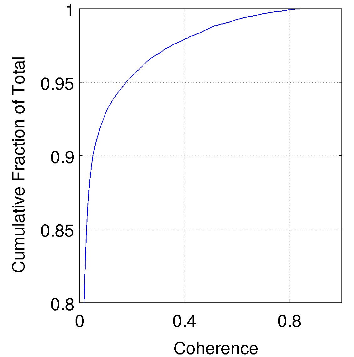
Figure 11: Empirical cumulative distribution functions of pairwise inner product magnitudes for dictionaries ${{\mathcal{D}}}_{\textrm{\small Africa},36,1}$ (left) and ${{\mathcal{D}}}_{\textrm{\small Africa},36,2}$ (right). In both cases, approximately $95\%$ of pairwise inner products have a value within $\pm 0.1$.

The requirement that the dictionary elements form an orthogonal basis is less important than the property of mutual incoherence. This we identify when the inner product between pairs of elements is almost always very low. Figure 10 shows that the two tree constructions on continental Africa have good incoherency properties: most dictionary element pairs are nearly orthogonal. As can be seen from Figure 10a, most pairwise inner products are nearly zero. More specifically, as expected, dictionary elements ${(j,1)}$, ${(2j,1)}$, ${(2j+1,1)}$, ${(2(2j),1)}$, ${(2(2j)+1,1)}$, ${(2(2j+1),1)}$, ${(2(2j+1)+1,1),\ldots}$, tend to have large inner products, while those with non-overlapping borders do not. This exact property is also visible in the two diagonal submatrices of Figure 10b. In the off-diagonals, due to the orthonormality of the construction, elements of the form $(j,1)$ and $(j,2)$ are orthogonal. In contrast, due to the nature of the tree subdivision scheme, elements of the form $(2j,1)$ or $(2j+1,1)$ and $(j,2)$ have a large inner product. However, the number of connections between nodes and their ancestors is $\mathcal{O}(n\,[2^{H}H])$, while the total number of pairwise inner products is $\mathcal{O}([n2^{H}]^{2})$; and for reasonably sized values of $L$ the ratio of ancestral connections to pairwise inner products gets to be small, see Figure 11.

4 Conclusions

We have introduced two classes of spherical parameterizations and discussed their properties in the context of geophysical model analysis and representation. The first involved the porting of traditional Cartesian wavelet transforms to the sphere via a cubed-sphere mapping, with and without special consideration for the boundaries between the six chunks constituting the entire spherical surface. The second was a novel elaboration of the classical ideas of signal concentration on the sphere. Starting from optimally spatially concentrated bandlimited spherical “Slepian” functions, we construct a dictionary of functions occupying a binary tree, where the elements of the tree are successive levels of Slepian functions calculated for an increasingly subdivided spatial domain.

Both the wavelet bases and the Slepian tree frames that we discuss in this paper are flexible and efficient ways of studying the information content and spatiospectral structure of geophysical and cosmological data. But in both cases their utility will also be derived from using them in the parameterization of geophysical inverse problems. In ref. 1 we discuss an iterative algorithm that solves an inverse problem in seismic tomography while promoting sparsity in the cubed-sphere wavelet basis in which the unknown model is expressed. Ref. 2 explores the inverse problem of approximating bandlimited, heterogeneously concentrated, essentially multiscale functions on the sphere from their samples.

In this paper and elsewhere, we have shown by example that many geophysical signals are sparse in the wavelet and Slepian (tree) “bases”. To tackle large-scale and potentially ill-conditioned inverse problems, the sparsity of the solution should actively be encouraged. In either case the inverse problem comes down to minimizing a mixed $\ell_{2}$-$\ell_{1}$ functional of the form

$${\mathcal{F}}({\mathbf{w}})=\|{\mathbf{K}}\cdot{\mathbf{S}}\cdot{\mathbf{w}}-{\mathbf{d}}\|^{2}_{2}+2\lambda\|{\mathbf{w}}\|_{1},$$ (7)

whereby ${\mathbf{d}}$ is a data set, ${\mathbf{K}}$ a linear operator, and ${\mathbf{S}}$ a certain synthesis map that transforms the set of unknown coefficients ${\mathbf{w}}$ into the domain of ${\mathbf{K}}$. Thus, ${\mathbf{S}}$ could relate to the wavelet bases introduced in Section 2 or to the Slepian-tree dictionary introduced in Section 3. Numerical experiments conducted for a variety of experimental setups under geophysically realistic conditions have already indicated that both types of constructions will be amenable to solving inverse problems in geophysics and beyond. Further research will be reported elsewhere.

5 Acknowledgments

We thank Jean Charléty, Huub Douma, Massimo Fornasier, Guust Nolet, Phil Vetter, Cédric Vonesch and Sergey Voronin for valuable discussions throughout the past several years. FJS was supported by Princeton University account 195-2142 and by NSF grant EAR-1014606 to FJS. Portions of this research were supported by VUB-GOA grant 062 to ICD and IL, the FWO-Vlaanderen grant G.0564.09N to ICD and IL, and by NSF grant CMG-0530865 to ICD and others. IL. is Research Associate of the F. R. S.-FNRS (Belgium).

Figure 3: Wavelet and scaling coefficients (top), space-domain reconstructions after thresholding (middle), and “signed” histograms (bottom) of the wavelet and scaling coefficients of the “North American” face of the cubed-sphere version of the Earth’s topography, to a $2^{J}$ dyadic subdivision with $J=3$. We used preconditioned interval wavelet transforms. All coefficients were hard-thresholded, retaining only the 15% largest coefficients by absolute value. In the top row, the locations of zeroed coefficients are rendered white; those are also captured by the white bars in the histograms. The root mean squared (rms) error of the reconstruction after thresholding is indicated as a percentage of the signal rms. Tick marks on the color bars identify the $5^{\mathrm{th}}$, $50^{\mathrm{th}}$ and $95^{\mathrm{th}}$ percentile of the coefficients or the spatial reconstructions after thresholding, respectively. Interior ticks on the histograms roughly coincide with these same percentiles as applied to either the positive and negative coefficients when expressed on a logarithmic scale. Histograms for the positive coefficients point up and have ordinates in positive percentages, histograms for the negative coefficients point down and have ordinates in negative percentages; these percentages are with respect to the total number of positive and negative coefficients. The blue and red shaded areas of the histograms reflect the coefficients retained at the global $85^{\mathrm{th}}$ thresholding level.

Figure 6: The binary tree subdivision scheme and associated dictionary ${{\mathcal{D}}}_{{{\mathcal{R}}},L}$ for the multiscale Slepian tree transform. We define the top-level region ${{\mathcal{R}}}$ as ${{\mathcal{R}}}^{(1)}$ and the generic subsets ${{\mathcal{R}}}^{\prime}$ as $R^{(j)}$.

References

- [1] F. J. Simons, I. Loris, G. Nolet, I. C. Daubechies, S. Voronin, P. A. Vetter, J. Charléty, and C. Vonesch, “Solving or resolving global tomographic models with spherical wavelets, and the scale and sparsity of seismic heterogeneity,” Geophys. J. Int. , p. in the press, 2011.
- [2] E. Brevdo, Efficient representations of signals in nonlinear signal processing with applications to inverse problems. PhD thesis, Princeton University, 2011.
- [3] I. Loris, G. Nolet, I. Daubechies, and F. A. Dahlen, “Tomographic inversion using -norm regularization of wavelet coefficients,” Geophys. J. Int. 170(1), pp. 359–370, doi: 10.1111/j.1365–246X.2007.03409.x, 2007.
- [4] I. Loris, H. Douma, G. Nolet, I. Daubechies, and C. Regone, “Nonlinear regularization techniques for seismic tomography,” J. Comput. Phys. 229(3), pp. 890–905, doi: 10.1016/j.jcp.2009.10.020, 2010.
- [5] C. Ronchi, R. Iacono, and P. S. Paolucci, “The “Cubed Sphere”: A new method for the solution of partial differential equations in spherical geometry,” J. Comput. Phys. 124, pp. 93–114, doi: 10.1006/jcph.1996.0047, 1996.
- [6] D. Komatitsch and J. Tromp, “Spectral-element simulations of global seismic wave propagation — I. Validation,” Geophys. J. Int. 149, pp. 390–412, 2002.
- [7] D. Slepian and H. O. Pollak, “Prolate spheroidal wave functions, Fourier analysis and uncertainty — I,” Bell Syst. Tech. J. 40(1), pp. 43–63, 1961.
- [8] H. J. Landau and H. O. Pollak, “Prolate spheroidal wave functions, Fourier analysis and uncertainty — II,” Bell Syst. Tech. J. 40(1), pp. 65–84, 1961.
- [9] D. Slepian, “Prolate spheroidal wave functions, Fourier analysis and uncertainty — IV: Extensions to many dimensions; generalized prolate spheroidal functions,” Bell Syst. Tech. J. 43(6), pp. 3009–3057, 1964.
- [10] F. J. Simons and D. V. Wang, “Spatiospectral concentration in the Cartesian plane,” Intern. J. Geomath. 2(1), pp. 1–36, doi: 10.1007/s13137–011–0016–z, 2011.
- [11] A. Albertella, F. Sansò, and N. Sneeuw, “Band-limited functions on a bounded spherical domain: the Slepian problem on the sphere,” J. Geodesy 73, pp. 436–447, 1999.
- [12] M. A. Wieczorek and F. J. Simons, “Localized spectral analysis on the sphere,” Geophys. J. Int. 162(3), pp. 655–675, doi: 10.1111/j.1365–246X.2005.02687.x, 2005.
- [13] F. J. Simons, F. A. Dahlen, and M. A. Wieczorek, “Spatiospectral concentration on a sphere,” SIAM Rev. 48(3), pp. 504–536, doi: 10.1137/S0036144504445765, 2006.
- [14] F. J. Simons and F. A. Dahlen, “A spatiospectral localization approach to estimating potential fields on the surface of a sphere from noisy, incomplete data taken at satellite altitudes,” in Wavelets XII, D. Van de Ville, V. K. Goyal, and M. Papadakis, eds., 6701, pp. 670117, doi: 10.1117/12.732406, SPIE, 2007.
- [15] F. J. Simons, J. C. Hawthorne, and C. D. Beggan, “Efficient analysis and representation of geophysical processes using localized spherical basis functions,” in Wavelets XIII, V. K. Goyal, M. Papadakis, and D. Van de Ville, eds., 7446, pp. 74460G, doi: 10.1117/12.825730, SPIE, 2009.
- [16] P. Schröder and W. Sweldens, “Spherical wavelets: Efficiently representing functions on the sphere,” Computer Graphics Proceedings (SIGGRAPH 95) 22, pp. 161–172, doi: 10.1145/218380.218439, 1995.
- [17] F. J. Narcowich and J. D. Ward, “Nonstationary wavelets on the m-sphere for scattered data,” Appl. Comput. Harmon. Anal. 3, pp. 324–336, 1996.
- [18] J.-P. Antoine, L. Demanet, L. Jacques, and P. Vandergheynst, “Wavelets on the sphere: implementation and approximations,” Appl. Comput. Harmon. Anal. 13, pp. 177–200, 2002.
- [19] M. Holschneider, A. Chambodut, and M. Mandea, “From global to regional analysis of the magnetic field on the sphere using wavelet frames,” Phys. Earth Planet. Inter. 135, pp. 107–124, 2003.
- [20] W. Freeden and V. Michel, “Orthogonal zonal, tesseral and sectorial wavelets on the sphere for the analysis of satellite data,” Adv. Comput. Math. 21(1–2), pp. 181–217, 2004.
- [21] N. L. Fernández and J. Prestin, “Interpolatory band-limited wavelet bases on the sphere,” Constr. Approx. 23, pp. 79–101, doi: 10.1007/s00365–005–0601–1, 2006.
- [22] A. A. Hemmat, M. A. Dehghan, and M. Skopina, “Ridge wavelets on the ball,” J. Approx. Theory 136(2), pp. 129–139, 2005.
- [23] M. Schmidt, S.-C. Han, J. Kusche, L. Sanchez, and C. K. Shum, “Regional high-resolution spatiotemporal gravity modeling from GRACE data using spherical wavelets,” Geophys. Res. Lett. 33(8), pp. L0840, doi: 10.1029/2005GL025509, 2006.
- [24] J. L. Starck, Y. Moudden, P. Abrial, and M. Nguyen, “Wavelets, ridgelets and curvelets on the sphere,” Astron. Astroph. 446, pp. 1191–1204, 2006.
- [25] J. D. McEwen, M. P. Hobson, D. J. Mortlock, and A. N. Lasenby, “Fast directional continuous spherical wavelet transform algorithms,” IEEE Trans. Signal Process. 55(2), pp. 520–529, 2007.
- [26] Y. Wiaux, J. D. McEwen, and P. Vielva, “Complex data processing: Fast wavelet analysis on the sphere,” J. Fourier Anal. Appl. 13(4), pp. 477–493, 10.1007/s00041–006–6917–9, 2007.
- [27] C. Lessig and E. Fiume, “SOHO: Orthogonal and symmetric Haar wavelets on the sphere,” ACM Trans. Graph. 27(1), pp. 4, doi: 10.1145/1330511.1330515, 2008.
- [28] F. Bauer and M. Gutting, “Spherical fast multiscale approximation by locally compact orthogonal wavelets,” Intern. J. Geomath. 2(1), pp. 69–85, doi: 10.1007/s13137–011–0015–0, 2011.
- [29] I. Daubechies, “Orthonormal bases of compactly supported wavelets,” Comm. Pure Appl. Math. 41, pp. 909–996, 1988.
- [30] A. Cohen, I. Daubechies, and J. Feauveau, “Biorthogonal bases of compactly supported wavelets,” Comm. Pure Appl. Math. 45, pp. 485–560, doi: 10.1002/cpa.3160450502, 1992.
- [31] A. Cohen, I. Daubechies, and P. Vial, “Wavelets on the interval and fast wavelet transforms,” Appl. Comput. Harmon. Anal. 1, pp. 54–81, 1993.
- [32] S. Mallat, A Wavelet Tour of Signal Processing, The Sparse Way, Academic Press, San Diego, Calif., 3 ed., 2008.
- [33] L. I. Rudin, S. Osher, and E. Fatemi, “Nonlinear total variation based noise removal algorithms,” Physica D 60(1–4), pp. 259–268, doi: 10.1016/0167–2789(92)90242–F, 1992.
- [34] D. C. Dobson and F. Santosa, “Recovery of blocky images from noisy and blurred data,” SIAM J. Appl. Math. 56(4), pp. 1181–1198, 1996.
- [35] A. Chambolle and P.-L. Lions, “Image recovery via total variation minimization and related problems,” Numer. Math. 76(2), pp. 167–188, 1997.
- [36] J. Trampert and R. D. van der Hilst, “Towards a quantitative interpretation of global seismic tomography,” in Earth’s Deep Mantle: Structure, Composition, and Evolution, R. D. van der Hilst, J. Bass, J. Matas, and J. Trampert, eds., Geophysical Monograph 160, pp. 47–62, Amer. Geophys. Union, Washington, D. C., 2005.
- [37] H. Tkalčić and B. Romanowicz, “Short scale heterogeneity in the lowermost mantle: insights from PcP-P and ScS-S data,” Earth Planet. Sci. Lett. 201(1), pp. 57–68, doi: 10.1016/S0012–821X(02)00657–X, 2002.
- [38] R. L. Saltzer, R. D. van der Hilst, and H. Kárason, “Comparing P and S wave heterogeneity in the mantle,” Geophys. Res. Lett. 28(7), pp. 1335–1338, 2001.
- [39] F. Deschamps and J. Trampert, “Mantle tomography and its relation to temperature and composition,” Phys. Earth Planet. Inter. 140(4), pp. 277–291, doi: 10.1016/j.pepi.2003.09.004, 2003.
- [40] A. Beck and M. Teboulle, “A Fast Iterative Shrinkage-Thresholding Algorithm for linear inverse problems,” SIAM J. Imag. Sci. 2(1), pp. 183–202, doi: 10.1137/080716542, 2009.
- [41] F. J. Simons and F. A. Dahlen, “Spherical Slepian functions and the polar gap in geodesy,” Geophys. J. Int. 166, pp. 1039–1061, doi: 10.1111/j.1365–246X.2006.03065.x, 2006.
- [42] P. A. Wedin, “On angles between subspaces of a finite dimensional inner product space,” Matrix Pencils 973, pp. 263–285, doi: 10.1007/BFb0062107, 1983.
- [43] R. Montelli, G. Nolet, F. A. Dahlen, and G. Masters, “A catalogue of deep mantle plumes: New results from finite-frequency tomography,” Geochem. Geophys. Geosys. 7, pp. Q11007, doi: 10.1029/2006GC001248, 2006.
- [44] J. Ritsema, A. A. Deuss, H. J. van Heijst, and J. H. Woodhouse, “S40RTS: a degree-40 shear-velocity model for the mantle from new Rayleigh wave dispersion, teleseismic traveltime and normal-mode splitting function measurements,” Geophys. J. Int. 184, pp. 1223–1236, doi: 10.1111/j.1365–246X.2010.04884.x, 2010.