Mixed Ising ferrimagnets with next-nearest neighbour couplings on square lattices

Abstract

We study Ising ferrimagnets on square lattices with antiferromagnetic exchange couplings between spins of values S=1/2 and S=1 on neighbouring sites, couplings between S=1 spins at next–nearest neighbour sites of the lattice, and a single–site anisotropy term for the S=1 spins. Using mainly ground state considerations and extensive Monte Carlo simulations, we investigate various aspects of the phase diagram, including compensation points, critical properties, and temperature dependent anomalies. In contrast to previous belief, the next–nearest neighbour couplings, when being of antiferromagnetic type, may lead to compensation points.

J. Phys.: Condens. Matter

1 Introduction

Mixed spin ferrimagnetic Ising models have been studied for some time, with a renewed interest, especially, in connection with ’compensation points’, see, for instance, [1-11]. These points occur at temperatures, below the critical temperature, at which the sublattice magnetizations cancel exactly, giving zero total moment. As the temperature is tuned through such a point the total magnetization changes sign, which may be used in technological applications, most notably in magnetic recording.

One of the simplest such models consists of classical Ising spins S=1/2 and S=1 on a square or simple cubic lattice with the spins of different type being located on neighbouring sites of the lattice. Its Hamiltonian may be written in the form

$${\cal H}=J_{1}\sum_{\langle i,j\rangle}{\sigma_{i}S_{j}}+D\sum_{j\in B}{S_{j}}^{2}$$ (1)

where $J_{1}>0$ denotes the antiferromagnetic coupling between spins $\sigma_{i}=\pm 1/2$ on the sites of sublattice ’A’, and neighbouring spins $S_{j}=1,0,-1$ on sites forming the sublattice ’B’. Then, spins on each sublattice tend to order ferromagnetically, with opposite sign for the two types of spins. $D$ is the strength of a single–site anisotropy (or crystal–field) term acting only on the S=1 spins of sublattice B.

One may also choose $\sigma_{i}=\pm 1$ rather than $\pm 1/2$. The change has to be taken into account when calculating sublattice magnetizations and defining the compensation point. Otherwise, the modified convention simply amounts to a rescaling of the exchange coupling [5, 10].

The mixed spin Ising model, eq. (1), is known, see, e.g., [3, 5, 10], to lead to compensation points for simple cubic lattices, in accordance with mean–field theory [2], but not for square lattices, in contrast to mean–field theory. As has been observed already some years ago by Buendia and Novotny [5, 12], compensation points may occur on square lattices, when adding a (ferromagnetic) coupling between next–nearest neighbouring (nnn) spins on the A sublattice. On the other hand, the authors did not find any evidence for compensation points, when considering nnn couplings for B spins, instead of the ones for A spins.

In the following article we shall challenge the latter suggestion, which seems to have been taken for granted by others, see, e.g., [7]. Indeed, based on extensive Monte Carlo (MC) simulations, we shall present clear evidence for compensation points due to nnn antiferromagnetic interactions between B, or S=1, spins on the square lattice. In fact, the effect is not easy to identify.

The outline of the article is as follows. In section 2, to set the scene for the following parts, we define the model with nnn couplings between S=1 spins, discuss its ground states, and describe details of the simulations. The following section deals with the compensation points. In section 4, MC results on critical properties and temperature dependent anomalies of the model will be presented. A brief summary is given in the final section.

2 Model, ground states, and simulations

We shall study the following mixed spin Ising model on a square lattice

$${\cal H}=J_{1}\sum_{\langle i,j\rangle}{\sigma_{i}S_{j}}+D\sum_{j\in B}{S_{j}}^{2}-J_{2}\sum_{\langle i,j\rangle\in B}{S_{i}S_{j}}$$ (2)

with antiferromagnetic nearest neighbour couplings, $J_{1}>0$ between A spins, $\sigma_{i}=\pm 1$, and B spins, $S_{j}=0,\pm 1$, a crystal–field term of strength $D$ acting on the B spins, and nnn couplings, $J_{2}$, between B spins. Note that we set A spins equal to $\pm 1$, in accordance with previous work [5, 10]. To identify possible compensation points, care is then needed in defining the magnetization of the sublattice A, see above and below.

To determine the ground states of the model in the ($D/J_{1}$,$J_{2}/J_{1}$) plane, we first select, like before [5, 12, 13], the structures which are stable among the ones described by 2$\times$2 cells of spins on the square lattice. One readily observes the possibility of degenerate ground states, eventually with indefinitely large unit cells. Finally, we check the tentative ground state structures by monitoring spin configurations at very low temperatures obtained from careful cooling MC runs for lattices of various sizes. The resulting ground state phase diagram is depicted in figure 1.

The phase diagram at vanishing temperature, $T=0$, comprises four structures. The antiferromagnetic (AF) structure is stable for ferromagnetic or weakly antiferromagnetic nnn couplings, $J_{2}$, and negative or sufficiently small positive values of the crystal field, $D$. The spins on each of the two sublattices order ferromagnetically, $\pm 1$, with opposite sign on the sublattices A and B.

In two of the remaining other three ground states, S=1 spins may be in the state 0, due to the single–site anisotropy term, $D$. Actually, for sufficiently large values of $D$, all spins of the sublattice B are in state 0. We abbreviate the resulting structure as ’0II’. The structure is highly degenerate, with each A spin being either $-1$ or 1, leading to a $2^{N_{A}}$–fold degeneracy for $N_{A}$ sites on the sublattice A. In contrast, in the ’0I’ structure, see figure 1, only half of the S=1 spins are in the state 0. They form, on the sublattice B, in the standard Wood’s notation for overlayers [14], a periodic c($2\times 2$) superlattice. The other half of the spins on the B sites are ferromagnetically ordered, $\pm 1$. The spins on the sublattice A are ferromagnetically ordered as well, with opposite sign, compared to that of the B spins.

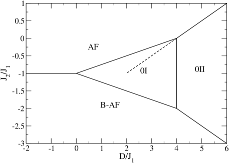
Figure 1: Ground state phase diagram of the mixed spin model, eq. (2), on a square lattice, with solid lines separating the different phases. The dashed line in the 0I phase refers to equation (7), see text.

In the fourth ground state structure, all spins on the sublattice B are antiferromagnetically aligned, due to the dominant antiferromagnetic nnn coupling, J₂. The structure may be abbreviated as B–AF. Each spin on the sublattice A may be either $-1$ or 1, leading, as for 0II, to a large degeneracy.

Note that there may be additional degeneracies at borderlines between different ground state structures [10].

To determine thermal properties of the model, (2), we mainly perform MC simulations, using the Metropolis algorithm with single–spin flips, providing, indeed, the required accuracy, so that there is no need to apply other techniques like cluster–updates or the Wang–Landau approach [15]. We consider lattices with $L$x$L$ sites, employing full periodic boundary conditions. $L$ ranges from 4 to 120, to study finite–size effects. Typically, we do runs of $5\times 10^{6}$ to $10^{7}$ Monte Carlo steps per spin, where averages and error bars may be obtained from evaluating a few of such runs, using different random numbers. These quite long runs lead to reliable data, as before [10]. The estimated errors are usually smaller than the sizes of the symbols in the figures, and they are shown there only in a few cases.

We record the energy per site, $E$, the specific heat, $C$, both from the energy fluctuations and from differentiating $E$ with respect to the temperature, and the absolute values of the sublattice magnetizations of the two sublattices

$$|m_{A}|=<|\sum_{A}{\sigma_{i}}|>/(2(L^{2}/2))$$ (3)

and

$$|m_{B}|=<|\sum_{B}{S_{j}}|>/(L^{2}/2)$$ (4)

as well as the absolute value of the staggered magnetization of sublattice B, describing the ordering for the B–AF structure,

$$|m^{st}_{B}|=<|\sum_{B^{+}}{S_{i}}-\sum_{B^{-}}{S_{j}}|>/(L^{2}/2)$$ (5)

with B^+,- denoting an obvious bipartition of sublattice B. The brackets $<>$ denote the thermal average. Note the factor of 1/2 in the definition of $|m_{A}|$, taking into account the correct length of the S=1/2 spins, so that $|m_{A}(T=0)|=1/2$ for the ferromagnetic ground state of sublattice A. In addition, the corresponding sublattice (staggered) susceptibilities, $\chi_{A}$, $\chi_{B}$, and $\chi_{B}^{st}$, have been computed from the fluctuations of the (staggered) sublattice magnetizations. We also analyse the fourth–order cumulant of various (sublattice) order parameters, the Binder cumulant [16], defined by

$$U=1-<m^{4}>/(3<m^{2}>^{2})$$ (6)

with $<m^{2}>$ and $<m^{4}>$ being the second and fourth moment of (staggered) magnetizations of sublattice A or B. Finally, we monitor typical equilibrium Monte Carlo configurations, illustrating the microscopic behaviour of the system and providing, e.g., evidence for the ground states structures, as mentioned above.

To test the accuracy of the simulations, we compared our MC data to those of previous accurate numerical work and to exact results by enumerating all possible configurations for small lattices with $L=4$ [5, 10].

3 Compensation points

Compensation points occur at temperatures $T_{comp}$, where both sublattice magnetizations cancel each other, with a vanishing total magnetization. In finite systems, as one is studying in MC simulations, a convenient and efficient way [5] to locate such points is to use the crossing condition $|m_{A}|(T_{comp})=|m_{B}|(T_{comp})$. At low temperatures sufficiently far below the phase transition, finite–size effects are expected to be very weak, because there the compensation effect is not related to critical phenomena.

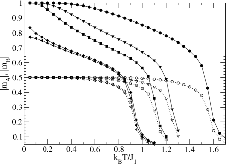
Figure 2: Sublattice magnetizations $|m_{A}|$ (open symbols, dotted lines) and $|m_{B}|$ (full symbols, solid lines) at fixed $D/J=3.0$ and varying $J_{2}/J_{1}$= 0.25 (circles), 0.0 (triangles down), $-0.1$ (squares), $-0.24$ (diamonds), and $-0.26$ (triangles left). Lattices of size $60^{2}$ are simulated.

In the AF ground state, one has $|m_{B}|(T=0)$=1, while $|m_{A}|(T=0)$= 1/2. Now, at non–zero temperatures, $|m_{B}|(T)$ may fall off quite rapidly due to antiferromagnetic couplings $J_{2}$ and due to a relatively large single–site anisotropy term, $D$, which favours flips of S=1 spins to state 0. Furthermore, at zero temperature, $|m_{B}|(T=0)$ drops from 1 to 1/2, when passing through the borderline between the AF and 0I ground states. Accordingly, one might speculate that compensation points, at low temperatures in the AF phase, may show up close to the AF–0I borderline at $T$=0. In fact, our preliminary mean–field calculations seem to suggest that lines of compensation points may spring from this AF–0I borderline.

However, in our MC simulations, investigating carefully several cases, we find no evidence for such compensation points in the AF phase. An example is depicted in figure 2. There, $D/J_{1}$ is fixed at 3.0, and $J_{2}/J_{1}$ is varied, from +0.25 to $-0.26$, so that the AF–0I border at $J_{2}/J_{1}$ = $-0.25$ is approached and crossed. One observes, that $|m_{B}|$ is always larger than $|m_{A}|$, albeit the difference between the two sublattice magnetizations may get quite small when decreasing $J_{2}$. MC data for lattices of fixed size, $L=60$, are displayed. The observation on the absence of compensation points in the AF phase also holds for other lattice sizes as well as for other values of $J_{2}/J_{1}$ and $D/J_{1}$.

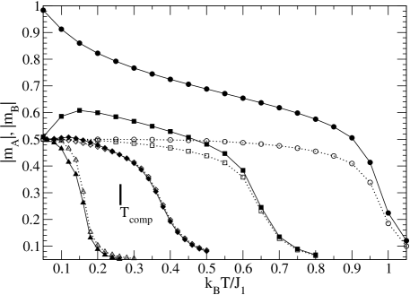
Figure 3: Sublattice magnetizations $|m_{A}|$ (open symbols, dotted lines) and $|m_{B}|$ (full symbols, solid lines) at fixed $J_{2}/J_{1}=-0.2$, and varying $D/J_{1}$= 3.0 (circles), 3.4 (squares), 3.57 (diamonds), and 3.7 (triangles up), simulating lattices of size $L$= 60. At $D/J_{1}$ =3.57, a compensation point shows up, $T_{comp}$.

On the other hand, compensation points will be argued below to occur in the 0I phase, for $J_{2}/J_{1}>-1.0$, arising at vanishing temperature from the line

$$J_{2}/J_{1}=-2+D/(2J_{1})$$ (7)

which is depicted as the dashed line in the ground state phase diagram, figure 1.

Let us first present numerical support for this claim, followed then by low temperature energy considerations backing it up. A numerical example is shown in figure 3, where, for lattices with $60^{2}$ sites, the temperature dependences of the sublattice magnetizations, $|m_{A}|$ and $|m_{B}|$, are shown at fixed nnn coupling, $J_{2}/J_{1}=-0.2$, and varying the strength of the single-site anisotropy term, $D/J_{1}$, from 3.0 to 3.7. Note that for this ratio of couplings, at $T=0$, the AF–0I border is at 3.2, and the origin, at vanishing temperature, of the line of compensation points would be, according to equation (7), at $D/J$= 3.6. As discussed in the context of figure 2, one observes that $|m_{B}|(T)$ is always larger than $|m_{A}|(T)$ when being in the AF phase. However, in the 0I phase, here, at $D/J_{1}$= 3.57, there seems to be a compensation point, with $k_{B}T_{comp}/J_{1}\approx 0.26$, clearly below the phase transition: At lower temperatures, $|m_{B}|$ is still larger than $|m_{A}|$, with reverse ordering at $T>T_{comp}$. By further increase of $D$, $D/J_{1}$= 3.7, $|m_{A}|(T)$ is larger than $|m_{B}|(T)$, at all temperatures up to $T_{c}$.

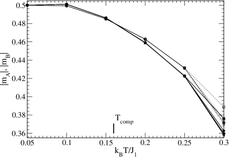
Figure 4: Sublattice magnetizations $|m_{A}|$ (open symbols, dotted lines) and $|m_{B}|$ (full symbols, solid lines) at $J_{2}/J_{1}=-0.2$ and $D/J_{1}$= 3.59, with lattice sizes $L$= 20 (squares), 40 (diamonds), 60 (triangles left), 80 (triangles down), and 120 (circles). The compensation point is located at $k_{B}T/J_{1}\approx 0.16$.

To establish numerically the presence of compensation points, careful finite–size analyses are required, as illustrated in figure 4. Here, MC data for various lattices sizes, with $L$ ranging from 20 to 120, are displayed, at $J_{2}/J_{1}=-0.2$ and $D/J_{1}$= 3.59, i.e. very close to the point, from which, according to (7), the line of compensation points may arise. In fact, a compensation point may be located at $k_{B}T_{comp}/J_{1}\approx 0.16$. Below that temperature, $|m_{B}|(T)$ supercedes $|m_{A}|(T)$, with finite–size dependences being extremely small. Then, at $T_{comp}$, a crossing of the two sublattice magnetizations occurs. The finite size effects are still very weak up to $k_{B}T/J_{1}\approx 0.25$, providing clear evidence on the existence of the compensation point in the thermodynamic limit.

Indeed, similar finite-size analyses allow one to locate the rather steeply rising line of compensation points, at fixed nnn couplings $J_{2}/J_{1}=-0.2$. Results on the compensation points, $T_{comp}$, are summarized in figure 5, together with estimates for the transition line, $T_{c}$, to the paramagnetic phase.

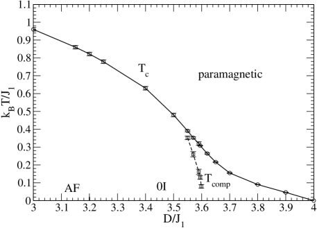
Figure 5: Phase boundary to the paramagnetic phase, $T_{c}$ (solid line), and compensation points, $T_{comp}$ (dashed line), at $J_{2}/J_{1}=-0.2$, varying $D/J_{1}$.

The critical line, $T_{c}$, has been determined by monitoring the size dependent positions of maxima in the specific heat $C$, in the susceptibility of the sublattice A, and in the intersection points of the Binder cumulant, especially, of sublattice A. The intersections of the Binder cumulant $U(L,T)$ for successive lattice sizes [16] turn out to have the smallest finite–size effects, thereby being most efficient in estimating the critical temperature.

The line of compensation points seems to start at zero temperature at $D/J_{1}$= 3.6 for $J_{2}/J_{1}=-0.2$, in agreement with equation (7). Furthermore, it extends only over quite a small region, with the compensation point coinciding with the critical point at about $D/J_{1}=3.52\pm 0.02$.

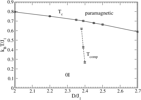
Figure 6: Phase boundary to the paramagnetic phase, $T_{c}$ (solid line), and compensation points, $T_{comp}$ (dashed line), at $J_{2}/J_{1}=-0.8$, varying $D/J_{1}$.

Let us now turn to the low temperature considerations leading to (7). Specifically, we consider, for the 0I structure, the one–spin flip excitations on sublattice B. For concreteness, we analyse ground states with spins being in state $-1$ or 0 on sublattice B, and in state 1 on sublattice A. Then there are four possible flips of S=1 spins, namely flipping a spin from its state 0 to the state (i) $-1$ or (ii) 1, or flipping a spin from its state $-1$ to state (iii) 0 or (iv) $+1$. Obviously, only flip (i) will increase the sublattice magnetization $|m_{B}|$ above its value at zero temperature, $|m_{B}|(T=0)=1/2$, while otherwise $|m_{B}|(T)$ will have a negative slope at low temperatures. Now, one may readily calculate the energies of all four elementary flips. One obtains that flip (i) costs the lowest energy either followed by flip (iii), when $D/J_{1}<2J_{2}/J_{1}+4$, or followed by flip (ii), when $J_{2}/J_{1}>-1.0$. Equation (7) is then obtained under the assumption, that an initial increase of $|m_{B}(T)|$ is needed to have a compensation point, with $|m_{B}|>|m_{A}|$ at sufficiently low temperatures. Otherwise, in the 0I phase, $|m_{A}|>|m_{B}|$ at all temperatures $0<T<T_{c}$, excluding a compensation point.

We further checked numerically the hypothesis, (7), in determining lines of compensation points by fixing the nnn coupling $J_{2}/J_{1}$ not only at $-0.2$, but also at $-0.4$ and $-0.8$, varying the strength of the single–site anisotropy term, $D/J_{1}$. Indeed, we observe compensation points in the 0I structure, which seem to arise, at zero temperature, from $D/J_{1}$= 3.2 at $J_{2}/J_{1}=-0.4$ and from $D/J_{1}$= 2.4 at $J_{2}/J_{1}=-0.8$, in agreement with (7). The latter case is displayed in figure 6.

Note that the range of values of $D/J_{1}$, in which there is a line of compensation points, shrinks appreciably as one decreases $J_{2}/J_{1}$. This may be seen by comparing figures 5 and 6. Thence, it becomes increasingly difficult to locate compensation points for lower values of $J_{2}/J_{1}$.

4 Phase transitions and anomalies

While mixed spin Ising models are of much interest because of the potential presence of compensations points, they may exhibit other intriguing thermal properties as well.

We shall focus on two aspects, the characterization of the phase transitions associated with the various ground states, and anomalies in the temperature dependence, especially, of the sublattice magnetization and the specifc heat $C$.

One expects that there is no phase transition associated with the highly degenerate 0II ground state for the following reasons: At zero temperature, all spins of sublattice B are in state 0, while each spin of sublattice A may be either $-1$ or 1. The single–site anisotropy term, favouring the spin state 0 on sublattice B, does not support long–range order, in close analogy to the situation in the Blume–Capel model [17]. The spins on sublattice A act merely like a fluctuating random field, and may not lead to a phase transition neither. In fact, our MC data, for various quantities, like the specific heat $C$ or the probability to encounter a spin in state 0, give no indication for singular thermal behaviour.

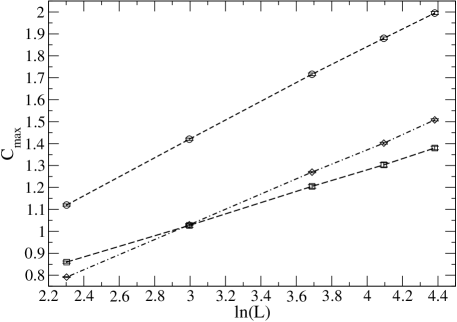
Figure 7: Height of the critical maximum of the specific heat, $C_{max}$ versus logarithm of the lattice size, $\ln L$, for $L$= 10, 20, 40, 60, and 80 at (a) (circles) $J_{2}/J_{1}=-0.3$, $D/J_{1}$ = 1.5, (b) (squares) $J_{2}/J_{1}=-1.0$, $D/J_{1}$= 1.5, and (c) (diamonds) $J_{2}/J_{1}=-1.5$, $D/J_{1}$= 2.5. The three cases refer to the (a) AF, (b) 0I, and (c) B–AF structures.

In case of the other three ground states, AF, 0I, and B–AF, we determine the universality class [18, 19] by analysing specific heat and susceptibilities. In particular, we monitor the size, $L$, dependence of that maximum of the specific heat, $C_{max}(L)$, which goes over into a singularity in the thermodynamic limit, $L\rightarrow\infty$ (note that there may be other maxima as will be discussed below in the context of anomalies). Furthermore, we study the size dependence of the maxima in (sublattice) susceptibilities. For the AF and 0I structures, we focus on $\chi_{A,max}(L)$. For the B–AF structure, we record the staggered susceptibility of the antiferromagnetically ordered sublattice B, $\chi^{st}_{B,max}(L)$. In all three cases, the critical behaviour is found to be consistent with having phase transitions in the universality class of the standard two–dimensional Ising model.

Typical MC results on the size, $L$, dependence of maxima in the specific heat, $C_{max}$, are depicted in figure 7. For all three types of ground states, AF, 0I as well as B–AF, one approaches to a good degree, already for lattices of moderate sizes, the form $C_{max}\propto\ln L$, being characteristic for the two–dimensional Ising universality class. Note that the prefactor in front of the logarithmic term depends strongly on $J_{2}/J_{1}$ and $D/J_{1}$. Certainly, such Ising–like critical behaviour may be expected in the AF case. In case of the B-AF phase, the spins on sublattice B order antiferromagnetically, with the A spins providing effectively a randomly fluctuating field, which may be argued to be irrelevant for the universality class. Finally, in the 0I case, the Ising–like criticality may be understood by the ferromagnetic order of the spins on sublattice A.

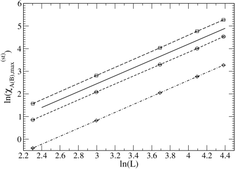
Figure 8: Log–log plot for maxima of (staggered) sublattice susceptibilities $\chi_{max}$ versus lattice size $L$ for the AF, 0I, and B–AF cases, with the same parameters and notation as in figure 7. In case of AF and 0I structures, $\chi_{A,max}$, in case of the B–AF structure, $\chi_{B,max}^{st}$ is recorded. For comparison, the solid line shows $\chi_{max}\propto L^{7/4}$.

The analysis of the susceptibilies confirms the findings on the specific heat. Typical examples, for the same model parameters as in figure 7, are shown in figure 8. The size dependent maxima in the susceptibilities are observed to follow the form $\chi_{max}\propto L^{7/4}$, with rather small corrections, for all three cases, AF, 0I, and B–AF. This behaviour may be quantified by calculating the slope between successive points in the doubly logarithmic plot of the MC data. The resulting effective local critical exponent of the susceptibility is near 7/4, even for moderate lattice sizes. Thence, in all three cases, criticality seems to belong to the two–dimensional Ising universality class.

Care is needed when attempting to determine the universality class from the value of the critical Binder cumulant $U^{*}$= $U(T_{c},L\longrightarrow\infty)$, because that value is known to depend on boundary conditions, shape, and anisotropy of the correlations [16, 20, 21]. Note that in the cases we studied, its value seems to be close to that of the standard two–dimensional Ising model with periodic boundary conditions for lattices of square shape, $U^{*}\approx 0.6107$ [22]. However, the dependence, especially on anisotropy, may be very weak [20, 21], and a reliable analysis may require an exact or, at least, extremely accurate determination of the critical point. We therefore refrained from such an analysis here.

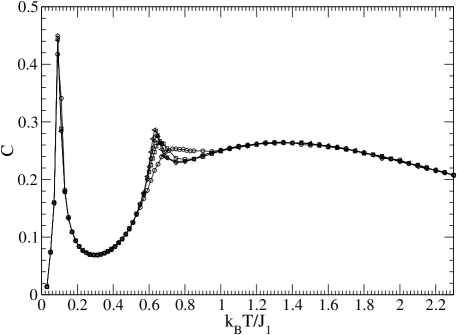
Figure 9: Specific heat $C$ as a function of temperature, $k_{B}T/J_{1}$, at $J_{2}/J_{1}=-0.2$ and $D/J=3.4$, simulating lattices of sizes $L$= 20 (circles), 40 (squares), 60 (diamonds), and 80 (triangles left).

Let us now turn to discussing anomalies, exhibiting intriguing non–monotonic temperature dependences, which are not related to phase transitions. Especially, we monitor the magnetizations of sublattice B, $|m_{B}|$, the specific heat $C$, and the thermally averaged occupancy of B sites with spins in the state 0, $p_{B}(0)$.

An example for such anomalies is the overshooting of $|m_{B}|(T)$ at low temperatures in the vicinity of the 0I ground state, illustrated in figures 2 and 3. As discussed above, the overshooting is related to decreasing the number of spins in state 0, by flipping such spins to, say, $-1$, costing minimal energy. Indeed, the anomaly in $|m_{B}|$ is monitored to be accompanied by a pronounced decrease in $p_{B}(0)$.

Anomalies may also occur in the specific heat, being caused either by a rapid increase or decrease in the number of S=1 spins in state 0. For instance, such an anomaly in $C$ has been observed before [10] in the AF phase at $J_{2}/J_{1}=0$, close to the 0II structure. There, monitoring $C(T)$, a three–peak–structure of the specific heat has been found, with a non-critical maximum at low temperatures, due to easy flips of spins in the state 0, followed, at higher temperature, by a strongly size dependent critical peak, and, at even larger temperature, another non–critical maximum, due to flipping of single spins for sublattices with rather large clusters of ’+’ or ’$-$’ spins.

We observe a similar thermal behaviour of the specific heat in the 0I phase, when turning on the nnn coupling, $J_{2}<0$. An example is depicted in figure 9, at $J_{2}/J_{1}=-0.2$ and $D/J_{1}$= 3.4. However, here the peak at lowest temperature, $T_{l}$, is due to a rather drastic decrease of B spins in state 0, which has been discussed above. Actually, by enhancing the strength of the single–site anisotropy term, $D/J_{1}=3.6$, the position of that peak, at $T_{l}$, shifts first to somewhat higher temperatures. It still corresponds to a lowering, with temperature, of the average number of 0’s for the sublattice B, $p_{B}(0)(T)$. When moving even closer to the 0II structure, $D/J_{1}$ = 3.8 and 3.9, $T_{l}$ tends to be shifted towards lower temperatures with increasing $D$. The peak position seems to follow the same dependence as for vanishing $J_{2}$ [10], namely $k_{B}T_{l}/J_{1}\propto 4-D/J_{1}$. As may be seen from monitoring $p_{B}(0)$, the peak is then, as in the limit $J_{2}=0$, due to an increase in the number of B spins in state 0 at low temperatures.

5 Summary

We have studied a mixed spin Ising model with antiferromagnetic couplings, $J_{1}$, between spins S= 1/2 and S= 1 on neighbouring sites of a square lattice, augmented by couplings, $J_{2}$, between spins S= 1 on next–nearest neighbouring sites of the lattice. An additional quadratic single–site anisotropy term, $D$, acts upon the S=1 spins. Based mainly on ground state considerations and on extensive standard Monte Carlo simulations, we have determined the ground state phase diagram in the ($D/J_{1},J_{2}/J_{1}$) plane and identified compensation points, types of phase transitions corresponding to different ground state structures as well as anomalies for various physical quantities.

In particular, compensation points are found to exist, in contrast to previous belief. They exist for antiferromagnetic nnn couplings, $J_{2}>-1.0$, in the 0I phase, springing, at zero temperature, from the line $J_{2}/J_{1}=-2+D/(2J_{1})$. Across that line, different types of one–spin flips on the S=1 sublattice cost lowest energy, accompanied by a change in the sign of the slope of the magnetization of that sublattice at low temperatures. At fixed value of $J_{2}/J_{1}$, the range, in $D/J_{1}$, of compensation points is quite narrow, becoming extremely small for decreasing nnn couplings, as we have shown by decreasing $J_{2}/J_{1}$ from $-0.2$ to $-0.8$.

The transition to the paramagnetic phase appears to be always in the universality class of the two–dimensional Ising model, with the critical maxima of the specific heat growing with lattice size, $L$, in a logarithmic fashion, and with the maxima of the appropriate (staggered) sublattice susceptibilities growing with lattice size proportionally to $L^{7/4}$. These results hold in case of AF, 0I, and B–AF ground states of the model. In case of the 0II ground state, there is no phase transition.

The model is observed to exhibit interesting anomalies by showing non–monotonic temperature dependences for various quantities, including sublattice magnetization and specific heat. The anomalies are typically caused by energetically favoured flips of S= 1 spins between the state 0 and a non–zero state.

In conclusion, our study provides clear evidence for non–expected compensation points in a rather simple mixed Ising model with antiferromagnetic next–nearest neighbour couplings between S=1 spins on a square lattice. Extensions to three dimensional lattices are well beyond the present study, and may be investigated in the future.

6 Acknowledgements

C E thanks the Department of Physics at the RWTH Aachen for the kind hospitality during his stay there. We thank Prof. Mark Novotny for a very useful discusssion as well as Dr. Mukul Laad for interesting conversations.

References

References

- [1] Néel L 1948 Ann. Phys. (Paris) 3 137
- [2] Kaneyoshi T and Chen J C 1991 J. Magn. Magn. Mater. 98 201
- [3] Zhang G-M and Yang C-Z 1993 Phys. Rev. B 48 9452
- [4] Bobák A and Jascur M 1995 Phys. Rev. B 51 11533
- [5] Buendia G M and Novotny M 1997 J. Phys.: Condens. Matter 9 5951
- [6] Oitmaa J and Zheng W-H 2003 Physica A 328 185
- [7] Godoy M, Leite V S, and Figueiredo W 2004 Phys. Rev. B 69 054428
- [8] Jascur M and Strecka J 2005 Condens. Matter Phys. 8 869
- [9] Oitmaa J and Enting I G 2006 J. Phys.: Condens. Matter 18 10931
- [10] Selke W and Oitmaa J 2010 J. Phys.: Condens. Matter 22 076004
- [11] Zukovic M and Bobák A 2010 Physica A 389 5402
- [12] Buendia G M and Novotny M A 1997 J. Phys. IV (C1) France 7 175
- [13] Buendia G M and Liendo J A 1997 J. Phys.: Condens. Matter 9 5439
- [14] Oura K, Lifshits V G, Saranin A A, Zotov A V and Katayama M 2003 Surface Science: An Introduction (Berlin: Springer)
- [15] Landau D P and Binder K 2005 A Guide to Monte Carlo Simulations in Statistical Physics (Cambridge: Cambridge University Press)
- [16] Binder K 1981 Z. Physik B 43 119
- [17] Blume M 1966 Phys. Rev. 141 517; Capel H W 1966 Physica (Utr.) 32 966
- [18] Fisher M E 1974 Rev. Mod. Phys. 46 597
- [19] Pelissetto A and Vicari E 2002 Phys. Rep. 368 549
- [20] Chen X S and Dohm V 2004 Phys. Rev. E 70 056136; Dohm V 2008 Phys. Rev. E 77 061128
- [21] Selke W and Shchur L N 2005 J. Phys. A: Math. Gen. 38 L739; Selke W 2006 Eur. Phys. J. B 51 223
- [22] Kamieniarz G and Blöte H W J 1993 J. Phys. A: Math. Gen 26 201