A relativistic model of the topological acceleration effect

Abstract

It has previously been shown heuristically that the topology of the Universe affects gravity, in the sense that a test particle near a massive object in a multiply connected universe is subject to a topologically induced acceleration that opposes the local attraction to the massive object. It is necessary to check if this effect occurs in a fully relativistic solution of the Einstein equations that has a multiply connected spatial section. A Schwarzschild-like exact solution that is multiply connected in one spatial direction is checked for analytical and numerical consistency with the heuristic result. The T¹ (slab space) heuristic result is found to be relativistically correct. For a fundamental domain size of $L$, a slow-moving, negligible-mass test particle lying at distance $x$ along the axis from the object of mass $M$ to its nearest multiple image, where $GM/c^{2}\ll x\ll L/2$, has a residual acceleration away from the massive object of $4\zeta(3)G(M/L^{3})\,x$, where $\zeta(3)$ is Apéry’s constant. For $M\sim 10^{14}M_{\odot}$ and $L\sim 10$ to $20{\mbox{$h^{-1}$ Gpc}}$, this linear expression is accurate to $\pm 10\%$ over $3{\mbox{$h^{-1}$ Mpc}}\,\lower 2.58334pt\hbox{$\buildrel<\over{\sim}$}\,x\,\lower 2.58334pt\hbox{$\buildrel<\over{\sim}$}\,2{\mbox{$h^{-1}$ Gpc}}$. Thus, at least in a simple example of a multiply connected universe, the topological acceleration effect is not an artefact of Newtonian-like reasoning, and its linear derivation is accurate over about three orders of magnitude in $x$.

1 Introduction

The topology of spatial sections of the Universe has been of interest since the foundations of relativistic cosmology (e.g., de Sitter, 1917; Friedmann, 1923, 1924; Lemaître, 1927; Robertson, 1935). However, astronomical measurements aimed at determining spatial topology have long suffered a theoretical disadvantage compared to curvature measurements. The latter are tightly related to another type of astronomical measurement (matter-energy density) via a well-established physical theory: general relativity. Some elementary work that might lead to a physical theory of cosmic topology has been carried out, by comparing certain characteristics of different manifolds (Seriu, 1996; Anderson et al., 2004) and by explorations of some elements of topology change in quantum gravity (e.g., Dowker and Surya, 1998), but these remain very distant from astronomical observations. Thus, most of the empirical work of the past few decades has been carried out with no theoretical constraints, apart from assuming Friedmann-Lemaître-Robertson-Walker (FLRW) cosmological models. For recent empirical analyses of the case for and against a multiply connected positively curved spatial section, in particular the Poincaré dodecahedral space S${}^{3}/I^{*}$, see Roukema and Kazimierczak (2011) and references therein. Theoretical developments could offer the possibility of new astronomical tests for cosmic topology.

For perfectly homogeneous solutions of the Einstein equations, i.e. FLRW models, if the sign of the curvature is determined empirically, only the covering space H³, $\mathbb{R}^{3}$, or S³, i.e. an apparent space containing many copies of the fundamental domain, can be inferred. The 3-manifold of comoving space itself, i.e. H${}^{3}/\Gamma$, $\mathbb{R}^{3}/\Gamma$, or S${}^{3}/\Gamma$, respectively, for a fundamental group (holonomy group) $\Gamma$, is not implied by the curvature. However, heuristic, Newtonian-like calculations have recently shown that the presence of a single inhomogeneity is enough to, in principle, distinguish different possible spaces of the same fixed curvature (Roukema et al., 2007; Roukema and Różański, 2009). The effect is a long-distance, globally induced acceleration term that opposes the local attraction to a massive object. Curiously, the effect, (hereafter, “topological acceleration”) is much weaker in the Poincaré dodecahedral space than in other spaces, hinting at a theoretical reason for selecting this space independent of the observational reasons published six years earlier. Other calculations of globally induced effects of the spatial topology of a fixed FLRW background include Infeld and Schild (1946) and Bernui et al. (1998).

Astronomical tests for cosmic topology are almost always based on the fact that photons from a point in comoving space can arrive at the observer by multiple paths (e.g. Roukema, 2002). In contrast, topological acceleration has the potential to provide tests of galaxy kinematics that could provide experimental constraints on cosmic topology independent of tests based on multiple imaging (of extragalactic objects or of cosmic microwave background temperature fluctuations). However, the calculations of the effect (Roukema et al., 2007; Roukema and Różański, 2009) did not use full solutions of the Einstein equations. The FLRW metric is an exact solution of the Einstein equations, but it can only by applied to the real Universe as a heuristic guide, since galaxies (inhomogeneities) exist. When this heuristic guide is used to interpret recent observational constraints, an accelerating scale factor and dark energy are inferred. That is, the latter appear to be artefacts of a heuristic approach (e.g. Célérier et al., 2010; Buchert and Carfora, 2003; Wiegand and Buchert, 2010). Similarly, since a heuristic, Newtonian-like approach was used to calculate the topological acceleration effect, the latter could, in principle, also be an artefact. Thus, it is important to check whether the effect really exists in the relativistic case of a $(3+1)$-dimensional spacetime with multiply connected spatial sections. Indeed, in reviews of cosmic topology (e.g., Ellis, 1971; Lachièze-Rey and Luminet, 1995; Luminet and Roukema, 1999; Levin, 2002; Rebouças and Gomero, 2004), the use of the exact (locally homogeneous) FLRW models has generally led to the inference that in a classical general relativistic model, spatially global topology should only constrain the curvature-related parameters of the metric (for methods, see e.g., Uzan et al., 1999; Roukema and Luminet, 1999; Bento et al., 2006; Rebouças and Alcaniz, 2006; Bento et al., 2006; Rebouças et al., 2006). This inference only becomes incorrect when the universe model contains at least one inhomogeneity.

Strictly speaking, from the point of view of differential geometry alone, astronomical tests for cosmic topology based on multiple imaging are degenerate. They do not distinguish a multiply connected space from a simply connected universal cover that happens to be populated by physically distinct objects located at appropriate positions in a perfectly regular tiling. Similarly, what we refer to here as “topological acceleration” could be interpreted as an effect of a perfectly regular tiling in a simply connected covering space. In this paper, we adopt the Schwarzschildian approach to lifting the degeneracy, “We would be much happier with the view that these repetitions are illusory, that in reality space has peculiar connection properties so that if we leave any one cube through a side, then we immediately reenter it through the opposite side,” (transl., Schwarzschild, 1900; Stewart et al., 1998) This is similar to the interpretation of what are normally claimed to be multiple, “gravitationally lensed” images of a single physical object as representing a single object rather than multiple objects that happen to mimic what is expected from a gravitational lensing hypothesis (e.g., Adam et al., 1989).

Here, we compare the heuristic calculation of Roukema et al. (2007) for T¹ (slab space, i.e. S${}^{1}\times\mathbb{R}^{2}$) to a limiting case of an exact, Schwarzschild-like solution which has a T¹ spatial section outside of the event horizon. This is a simpler 3-manifold than those that seem to be favoured by observations (as stated above, see Roukema and Kazimierczak, 2011, and references therein), with only one short dimension, and it only contains one massive object. Checking the existence of topological acceleration in this relativistic case does not guarantee corresponding results in more complicated cases, but it does open the prospect of generalisations. In Sect. 2.1 we list the simplifying assumptions for considering a test particle distant from the event horizon but much closer to the “first” copy of a massive object than to an “adjacent” copy. The metric in Weyl coordinates and related functions (Korotkin and Nicolai, 1994) are given in Sect. 2.2 for an analytical derivation and the numerical method is stated in Sect. 3.2 The analytical and numerical calculations are presented in Sect. 3.1 and Sect. 3.2, respectively, and a conclusion is given in Sect. 4.

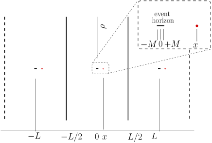
Figure 1: Event horizon of massive object of mass $M$ (dark line segment) and test particle (dot) in slab space T¹ of fundamental domain length $L$. In a 3-section of constant coordinate time $t$, the event horizon of the massive object is spherically symmetric in terms of the metric, but in the Weyl coordinates used here, it is a line segment extending from $-M$ to $+M$ in the $x$ direction, where $G=c=1$, and is of zero size in the radial coordinate $\rho$. The test particle is displaced a small distance from the massive object, i.e. $x\ll L/2$, but well outside the event horizon, i.e. $0<M\ll x$ (zoom) [Eq.(2)].

2 Method

For the Newtonian-like calculation, Fig. 3 of Roukema et al. (2007) illustrates the situation of a test particle at distance $x$ from a point object of mass $M$ in T¹, lying along the spatial geodesic of length $L$ from the massive object to itself. Defining $\epsilon:=x/L$ gives the topologically induced acceleration (Eq. (7), Roukema et al., 2007)

$$\ddot{x} = M\sum_{j=1}^{\infty}\left[\frac{1}{(jL-x)^{2}}-\frac{1}{(jL+x)^{2}}\right]\approx 4.8\frac{M\epsilon}{L^{2}}$$ (1)

when $\epsilon\ll 1$, adopting $G=1$.

2.1 Assumptions

A Schwarzschild-like solution of the Einstein equations has an event horizon, but behaviour close to the event horizon (or inside it) is not of interest here. Also, if the topological acceleration effect were to be analysed for its effects on galaxy dynamics, peculiar velocities would typically be of the order of $10^{-3}$c and very rarely exceed $10^{-2}$c. As in the earlier derivation of Eq. (1), we consider a test particle lying along the closed spatial geodesic joining the massive object to itself, i.e. having Weyl radial coordinate $\rho=0$.

Thus, in addition to adopting the conventions $G=c=1$, a $(-,+,+,+)$ metric, Greek spacetime indices $0,1,2,3$ and Roman space indices $1,2,3$, our assumptions become:

$$0<M\ll x\ll L/2,$$ (2)

$$\frac{\mathrm{d}x^{i}}{\mathrm{d}t}\ll 1\;\;\Rightarrow\;\;\frac{\mathrm{d}x^{i}}{\mathrm{d}\tau}\ll 1\,\lower 2.58334pt\hbox{$\buildrel<\over{\sim}$}\,\frac{\mathrm{d}t}{\mathrm{d}\tau},$$ (3)

$$\rho=0,$$ (4)

where $\tau$ is the proper time along the test particle’s world line $x^{\alpha}(\tau)$, and $t\equiv x^{0}$. The assumption of a low coordinate velocity implies a low 4-velocity spatial component [Eq. (3)].

2.2 Analytical approach

Korotkin and Nicolai (1994) presented a family of multiply connected exact solutions of the Einstein equations that includes a Schwarzschild-like solution with T¹ spatial sections outside of the event horizon. Figure 1 shows this solution in Weyl coordinates $x$ and $\rho$. Using Weyl coordinates and the Ernst potential, the metric is

$$\mathrm{d}s^{2}=-\mathrm{e}^{\omega}\mathrm{d}t^{2}+\mathrm{e}^{-\omega}\left[\mathrm{e}^{2k}(\mathrm{d}x^{2}+\mathrm{d}\rho^{2})+\rho^{2}\mathrm{d}\phi^{2}\right]$$ (5)

from Eq. (9) of Korotkin and Nicolai (1994), where $k$ and $\omega$ relate to an Ernst potential $\varepsilon$ defined on $\xi:=x+\mathrm{i}\rho$, with

$$\varepsilon_{0}(x,\rho):=\frac{\sqrt{(x-M)^{2}+\rho^{2}}+\sqrt{(x+M)^{2}+\rho^{2}}-2M}{\sqrt{(x-M)^{2}+\rho^{2}}+\sqrt{(x+M)^{2}+\rho^{2}}+2M}$$ (6)

$$\omega_{0}:=\ln\varepsilon_{0},\;a_{0}:=0,\;{{{a_{j\not=0}:=\frac{2M}{L\,|j|}}}}$$ (7)

$$\omega(x,\rho):=\sum_{j=-\infty}^{\infty}\left[\omega_{0}(x+jL,\rho)+a_{j}\right],\;\;\;\varepsilon:=\mathrm{e}^{\omega}$$ (8)

$$\partial_{\xi}k=2\mathrm{i}\rho\frac{\partial_{\xi}\varepsilon\partial_{\xi}\bar{\varepsilon}}{(\varepsilon+\bar{\varepsilon})^{2}},$$ (9)

from Eqs (13), (12), (5) and (7) of Korotkin and Nicolai (1994). The Ernst potential is real for this solution, so Eq. (9) gives

$$\partial_{\xi}k=\frac{1}{2}\mathrm{i}\rho\frac{(\partial_{\xi}\varepsilon)^{2}}{\varepsilon^{2}}=\frac{1}{2}\mathrm{i}\rho\left[\partial_{\xi}(\ln\varepsilon)\right]^{2}=\frac{1}{2}\mathrm{i}\rho(\partial_{\xi}\omega)^{2}.$$ (10)

Thus, at $\rho=0$, we have $\partial_{\xi}k=0$, i.e. $k$ is a constant along $\rho=0$. We choose $k(\rho=0)=0$, since any other value just implies a rescaling of units. Thus, the metric on $\rho=0$ is

$$\mathrm{d}s^{2}=-\mathrm{e}^{\omega}\mathrm{d}t^{2}+\mathrm{e}^{-\omega}\left(\mathrm{d}x^{2}+\mathrm{d}\rho^{2}+\rho^{2}\mathrm{d}\phi^{2}\right).$$ (11)

Defining the tangent vector $\vec{V}$ by components $V^{\alpha}:=\mathrm{d}x^{\alpha}/\mathrm{d}\tau$, the geodesic equation for the test particle is $\nabla_{V}\vec{V}=\vec{0}$, i.e.

$$\frac{\mathrm{d}^{2}x^{\alpha}}{\mathrm{d}\tau^{2}}+\Gamma^{\alpha}_{\;\;\beta\gamma}\frac{\mathrm{d}x^{\beta}}{\mathrm{d}\tau}\frac{\mathrm{d}x^{\gamma}}{\mathrm{d}\tau}=0,$$ (12)

where $\Gamma^{\alpha}_{\;\;\beta\gamma}$ are the Christoffel symbols of the second kind. Since a $(-,+,+,+)$ convention is used and low velocities are assumed [Eq. (3)], coordinate and proper time are related by

$$\mathrm{d}\tau^{2}=|g_{00}|\,(\mathrm{d}x^{0})^{2}=e^{\omega}\,\mathrm{d}t^{2},$$ (13)

giving the $x^{1}$ coordinate acceleration

$$\frac{\mathrm{d}^{2}x^{1}}{\mathrm{d}t^{2}}=\frac{\mathrm{d}^{2}x}{\mathrm{d}t^{2}}=e^{-\omega}\frac{\mathrm{d}^{2}x}{\mathrm{d}\tau^{2}}.$$ (14)

Given the conditions in Eqs. (2), (3), and (4) and the Ernst potential expressions in Eqs. (11), (6), (7), and (8), conversion to metric units of $x$ and $t$ would only modify this to second order. In Sect. 3.1, ${\mathrm{d}^{2}x}/{\mathrm{d}t^{2}}$ is evaluated.

2.3 Numerical approach

The Ernst potential expressions [Eqs (6), (7), and (8)] are used for numerical evaluation of Eq. (20) (below) by finite differencing over small intervals. A typical cluster of galaxies has a mass of $\sim 10^{14}M_{\odot}$, i.e. $M=4.78$ pc in length units, and the most massive clusters have masses up to about $10^{15}M_{\odot}$. Observational estimates of $L$ are in the range 10 to 20$h^{-1}$ Gpc (e.g. Roukema and Kazimierczak, 2011, and references therein). Thus, typical scales of $M/L$ of interest should be $M/L\sim 10^{-10}$ to $10^{-8}$. Since $M/x,M/L,$ and $x/L$ are small, the use of 53-bit–significand double-precision floating-point numbers is replaced by arbitrary precision arithmetic, for $10^{-10}<M/L<10^{-8}$. These calculations are presented in Sect. 3.2.

3 Results

3.1 Coordinate acceleration

Given that the test particle is far from the “close” copy of the event horizon and from “distant” copies [Eq. (2)], we have $|\Gamma^{\alpha}_{\;\;\beta\gamma}|\ll 1$. Together with Eq. (3), this implies that most of the terms in the sum in Eq. (12) are small terms of second order or higher, leaving

$$\frac{\mathrm{d}^{2}x^{\alpha}}{\mathrm{d}\tau^{2}}+\Gamma^{\alpha}_{\;\;00}\left(\frac{\mathrm{d}x^{0}}{\mathrm{d}\tau}\right)^{2}\approx 0.$$ (15)

Since the metric is static (and diagonal), we have

$$\Gamma^{\alpha}_{\;\;00}=\frac{1}{2}g^{\alpha\lambda}(\partial_{0}g_{\lambda 0}+\partial_{0}g_{0\lambda}-\partial_{\lambda}g_{00})=-\frac{1}{2}g^{\alpha\lambda}\partial_{\lambda}g_{00}.$$ (16)

Using Eq. (13), Eq. (15) becomes

$$\frac{\mathrm{d}^{2}x^{\alpha}}{\mathrm{d}\tau^{2}}=\frac{1}{2}\frac{g^{\alpha\lambda}}{|g_{00}|}\partial_{\lambda}g_{00}.$$ (17)

Since the metric is diagonal, we have $g^{xx}=(g_{xx})^{-1}=e^{+\omega}$ and

$$\frac{\mathrm{d}^{2}x^{1}}{\mathrm{d}\tau^{2}}=\frac{1}{2}\frac{g^{11}}{|g_{00}|}\partial_{1}g_{00},$$ (18)

i.e.,

$$\frac{\mathrm{d}^{2}x}{\mathrm{d}\tau^{2}}=\frac{1}{2}\frac{g^{xx}}{|g_{tt}|}\partial_{x}g_{tt}=\frac{1}{2}\frac{e^{\omega}}{e^{\omega}}(-\partial_{x}e^{\omega})=-\frac{1}{2}e^{\omega}\partial_{x}\omega.$$ (19)

Thus, from Eq. (14),

$$\frac{\mathrm{d}^{2}x}{\mathrm{d}t^{2}}=-\frac{1}{2}\partial_{x}\omega.$$ (20)

Substituting Eq (7) in Eq. (8a) [corresponding to (12) and (5) of Korotkin and Nicolai (1994), respectively]

$$\omega(x,\rho) = w_{0}(x,\rho)+\sum_{j=-\infty,j\not=0}^{\infty}\left[\omega_{0}(x+jL,\rho)+\frac{2M}{L\,|j|}\right].$$ (21)

This is the convergent solution found by Korotkin and Nicolai (1994). Dropping the $\rho$ dependence since we are interested in the $\rho=0$ axis, the derivative can be written using Eq. (7)

$$\partial_{x}\omega(x) = \partial_{x}\left[\ln\varepsilon_{0}(x)+\sum_{j=-\infty,j\not=0}^{\infty}\ln\varepsilon_{0}(x+jL)\right]$$

$$= \frac{\partial_{x}\varepsilon_{0}(x)}{\varepsilon_{0}(x)}+\sum_{j=1}^{\infty}\frac{\partial_{x}\varepsilon_{0}(x+jL)}{\varepsilon_{0}(x+jL)}+\sum_{j=1}^{\infty}\frac{\partial_{x}\varepsilon_{0}(x-jL)}{\varepsilon_{0}(x-jL)}$$

$$= \frac{\partial_{x}\varepsilon_{0}(x)}{\varepsilon_{0}(x)}+\sum_{j=1}^{\infty}\frac{\partial_{x}\varepsilon_{0}(x+jL)}{\varepsilon_{0}(x+jL)}-\sum_{j=1}^{\infty}\frac{\partial_{x}\varepsilon_{0}(jL-x)}{\varepsilon_{0}(jL-x)}$$

$$\approx {\partial_{x}\varepsilon_{0}(x)}+\sum_{j=1}^{\infty}{\partial_{x}\varepsilon_{0}(jL+x)}-\sum_{j=1}^{\infty}{\partial_{x}\varepsilon_{0}(jL-x)},$$

where the third equality follows from using $\partial_{x^{\prime}}\varepsilon_{0}(-x^{\prime})=-\partial_{x^{\prime}}\varepsilon_{0}(x^{\prime})$ [cf. Eq. (6)], and the approximation follows from using Eqs (2), (4), and $j\geq 1$ in Eq. (6).

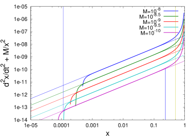
Figure 2: Topological acceleration $\mathrm{d}^{2}x/\mathrm{d}t^{2}+M/x^{2}$ as a function of coordinate distance $x$ from the “first” copy of the massive object of mass $M$, along the spatial geodesic joining the massive object to itself, using Eqs (6), (7), and (8) in Eq. (20), for $L=1$. The curves show masses from $M=10^{-10}$ to $10^{-8}$, from bottom to top, respectively, as labelled. The sloping lines show $4\zeta(3)(M/L^{3})x$. The vertical line at $x=0.5$ shows the halfway point to the “next” copy of the massive object. The vertical lines down to and up to the $M=10^{-10}$ curve show the range over which the linear approximation is valid to within $\pm 10\%$.

Table 1: Minimum and maximum distance $x$ for which the $4\zeta(3)(M/L^{3})\,x$ approximation is accurate to within 10% (cf. Fig. 2).^a

$$\begin{array}[]{l rrrrr}\hline\cr\hline\cr\rule{0.0pt}{10.76385pt}M&10^{-10}&3\times 10^{-10}&10^{-9}&3\times 10^{-9}&10^{-8}\\ \hline\cr\rule{0.0pt}{10.76385pt}\log_{10}x_{\min}&-3.94&-3.77&-3.54&-3.37&-3.14\\ \log_{10}x_{\max}&-0.63&-0.63&-0.63&-0.63&-0.63\\ \Delta\log_{10}x{{}^{\mathrm{b}}}&3.32&3.14&2.91&2.74&2.51\\ \hline\cr\end{array}$$

^aFor convenience, $L=1$.
^bRange in $\log_{10}x$.

For $0<M<x^{\prime}$, Eq. (6) simplifies to

$$\varepsilon_{0}(x^{\prime},0)=\frac{x^{\prime}-M}{x^{\prime}+M}.$$ (23)

Again defining $\epsilon:=x/L$, we then have

$$\rule{-12.91663pt}{0.0pt}\partial_{x}\omega(x)$$ (24)

$$\approx \frac{2M}{(x+M)^{2}}+\sum_{j=1}^{\infty}\frac{2M}{(jL+x+M)^{2}}-\sum_{j=1}^{\infty}\frac{2M}{(jL-x+M)^{2}}$$

$$\approx \frac{2M}{x^{2}}+\frac{2M}{L^{2}}\left(\sum_{j=1}^{\infty}\frac{1}{(j+\epsilon)^{2}}-\sum_{j=1}^{\infty}\frac{1}{(j-\epsilon)^{2}}\right)$$

$$\approx \frac{2M}{x^{2}}+\frac{2M}{L^{2}}\left[\sum_{j=1}^{\infty}\frac{1}{j^{2}}\left(1-\frac{2\epsilon}{j}\right)-\sum_{j=1}^{\infty}\frac{1}{j^{2}}\left(1+\frac{2\epsilon}{j}\right)\right]\rule{-12.91663pt}{0.0pt}$$

$$= \frac{2M}{x^{2}}-\frac{8M}{L^{2}}\epsilon\sum_{j=1}^{\infty}\frac{1}{j^{3}}$$

$$= \frac{2M}{x^{2}}-\frac{8\zeta(3)M}{L^{2}}\epsilon$$

where Eq. (2) is applied in the second and third lines, and $\zeta(3)$ is the Riemann zeta function evaluated at an argument of 3, i.e. Apéry’s constant.

Hence, using Eq. (20),

$$\frac{\mathrm{d}^{2}x}{\mathrm{d}t^{2}}\approx-\frac{M}{x^{2}}+\frac{4\zeta(3)M}{L^{2}}\,{\frac{x}{L}}\approx-\frac{M}{x^{2}}+\frac{4.8M}{L^{2}}\,{\frac{x}{L}}\;$$ (25)

i.e. the coordinate acceleration is the Newtonian acceleration towards the local copy of the massive object plus an opposing topological acceleration term matching Eq. (1), i.e. the expression derived earlier in Roukema et al. (2007).

3.2 Numerical check

For $10^{-10}<M<10^{-8}$, $L=1$, $|j|\leq 14$, and linear offsets of $\delta x=\pm 10^{-13}$ around each $x$ value, numerically convergent results were found using 100 bits in the significand. Figure 2 and Table 1 show that in this case, the linear approximation for the residual acceleration, $4\zeta(3)(M/L^{3})\,x$, is accurate to within 10% over about three orders of magnitude. Near the halfway point and at $x>0.5$, i.e. closer to the “next” image of the massive object than the “local” copy, the residual term defined in relation to the acceleration towards the “local” copy is clearly no longer small—it diverges as the test particle approaches the “next” copy. Thus, for $L\sim 10$ to $20$$h^{-1}$ Gpc, the linear expression should be accurate on scales of $3{\mbox{$h^{-1}$ Mpc}}\,\lower 2.58334pt\hbox{$\buildrel<\over{\sim}$}\,x\,\lower 2.58334pt\hbox{$\buildrel<\over{\sim}$}\,2{\mbox{$h^{-1}$ Gpc}}$ in a slab-space universe containing just one cluster of about $10^{14}M_{\odot}$.

4 Conclusion

The T¹ (slab space) heuristic result is found to exist in the limit of the Schwarzschild-like, exact, slab-space solution of the Einstein equations found by Korotkin and Nicolai (1994), with the same linear topological acceleration term as for the simpler calculation. For a fundamental domain size of $L$, a slow-moving [Eq. (3)], low-mass test particle lying at distance $x\ll L/2$ along the axis [$\rho=0$, Eq. (4)] from the object of positive mass $GM/c^{2}\ll x$ [Eq. (2)] to its nearest multiple image, the additional acceleration away from the massive object is $4\zeta(3)G(M/L^{3})\,x$ [Eq. (25)]. For a topological acceleration term away from a cluster of $\sim 10^{14}M_{\odot}$ and a Universe of size $L\sim 10$ to $20$$h^{-1}$ Gpc, the linear expression should be accurate over $3{\mbox{$h^{-1}$ Mpc}}\,\lower 2.58334pt\hbox{$\buildrel<\over{\sim}$}\,x\,\lower 2.58334pt\hbox{$\buildrel<\over{\sim}$}\,2{\mbox{$h^{-1}$ Gpc}}$ (Fig. 2, column with $M=3\times 10^{-10}$ in Table 1). Thus, at least in a simple example of a multiply connected universe, the topological acceleration effect is not an artefact of Newtonian-like reasoning. The linear term exists as an analytical limit of the relativistic model and as a good numerical approximation to it over several orders of magnitude of $x$.

This qualitatively suggests that the Newtonian-like derivations of the topological acceleration effect for well-proportioned FLRW models (Roukema and Różański, 2009), in which the Poincaré dodecahedral space is found to be uniquely well-balanced, might also be valid limits of fully relativistic Schwarzschild-like solutions with these spatial sections. Other extensions of the present work within the slab-space solution could include consideration of test particles with high coordinate velocities [violating Eq. (3)], or expanding (FLRW-like) solutions.

Although we have shown that topological acceleration exists theoretically, the effect is clearly weak over the range for which the linear expression is accurate. It is not clear how easy it might be to test the effect observationally. A possible method might follow from considering the effect as a feedback effect from global anisotropy to local anisotropy. Multiply connected FLRW models have usually been thought to be locally isotropic (the metric on a spatial section is isotropic) and globally anisotropic (some global tests differ depending on the chosen spatial direction). Here, we have confirmed that global anisotropy can imply a local acceleration effect. The effect is clearly anisotropic. The integration of this weak effect over a long period of time for individual particle trajectories or collapsing density perturbations might, in principle, give anisotropic long-term statistical behaviour that is strong enough to be detectable. Thus, the global anisotropy of a multiply connected space implies (at least in the case considered here) a weak, locally anisotropic dynamical effect. Whether or not the time-integrated effect could be strong enough to detect in observations of galaxy kinematics or cosmic web structure is a question worth exploring in future work.

References

- de Sitter (1917) de Sitter W 1917 MNRAS 78, 3–28.
- Friedmann (1923) Friedmann A 1923 Mir kak prostranstvo i vremya (The Universe as Space and Time) Leningrad: Academia.
- Friedmann (1924) Friedmann A 1924 Zeitschr. für Phys. 21, 326.
- Lemaître (1927) Lemaître G 1927 Annales de la Société Scientifique de Bruxelles 47, 49–59.
- Robertson (1935) Robertson H P 1935 ApJ 82, 284.
- Lemaître (1931) Lemaître G 1931 MNRAS 91, 483–490.
- Seriu (1996) Seriu M 1996 Phys. Rev. D 53, 6902, [arXiv:gr-qc/9603002v1].
- Anderson et al. (2004) Anderson M, Carlip S, Ratcliffe J G, Surya S and Tschantz S T 2004 CQG 21, 729, [arXiv:gr-qc/0310002].
- Dowker and Surya (1998) Dowker F and Surya S 1998 Phys. Rev. D 58, 124019, [arXiv:gr-qc/9711070].
- Roukema and Kazimierczak (2011) Roukema B F and Kazimierczak T A 2011 A&A 533, A11, [arXiv:1106.0727].
- Roukema et al. (2007) Roukema B F, Bajtlik S, Biesiada M, Szaniewska A and Jurkiewicz H 2007 A&A 463, 861–871, [arXiv:astro-ph/0602159].
- Roukema and Różański (2009) Roukema B F and Różański P T 2009 A&A 502, 27, [arXiv:0902.3402].
- Infeld and Schild (1946) Infeld L and Schild A E 1946 Physical Review 70, 410–425.
- Bernui et al. (1998) Bernui A, Gomero G I, Rebouças M J and Teixeira A F F 1998 Phys. Rev. D 57, 4699–4706, [arXiv:gr-qc/9802031].
- Roukema (2002) Roukema B F 2002 in V G Gurzadyan, R T Jantzen, & R Ruffini, ed., ‘The Ninth Marcel Grossmann Meeting’ Singapore: World Scientific pp. 1937–1938, [arXiv:astro-ph/0010189].
- Célérier et al. (2010) Célérier M, Bolejko K and Krasiński A 2010 A&A 518, A21+, [arXiv:0906.0905].
- Buchert and Carfora (2003) Buchert T and Carfora M 2003 Phys. Rev. Lett. 90(3), 031101, [arXiv:gr-qc/0210045].
- Wiegand and Buchert (2010) Wiegand A and Buchert T 2010 Phys. Rev. D 82(2), 023523, [arXiv:1002.3912].
- Ellis (1971) Ellis G F R 1971 General Relativity and Gravitation 2, 7–21.
- Lachièze-Rey and Luminet (1995) Lachièze-Rey M and Luminet J 1995 Phys. Rep. 254, 135, [arXiv:gr-qc/9605010].
- Luminet and Roukema (1999) Luminet J and Roukema B F 1999 in M Lachièze-Rey, ed., ‘NATO ASIC Proc. 541: Theoretical and Observational Cosmology. Publisher: Dordrecht: Kluwer,’ p. 117, [arXiv:astro-ph/9901364].
- Levin (2002) Levin J 2002 Phys. Rep. 365, 251–333, [arXiv:gr-qc/0108043].
- Rebouças and Gomero (2004) Rebouças M J and Gomero G I 2004 Braz. J Phys. 34, 1358, [arXiv:astro-ph/0402324].
- Uzan et al. (1999) Uzan J P, Lehoucq R and Luminet J P 1999 A&A 351, 766, [arXiv:astro-ph/9903155].
- Roukema and Luminet (1999) Roukema B F and Luminet J P 1999 A&A 348, 8–16, [arXiv:astro-ph/9903453].
- Bento et al. (2006) Bento M C, Bertolami O, Rebouças M J and Santos N M C 2006 Phys. Rev. D 73(10), 103521, [arXiv:astro-ph/0603848].
- Rebouças and Alcaniz (2006) Rebouças M J and Alcaniz J S 2006 MNRAS 369, 1693–1697, [arXiv:astro-ph/0603206].
- Bento et al. (2006) Bento M C, Bertolami O, Rebouças M J and Silva P T 2006 Phys. Rev. D 73(4), 043504, [arXiv:gr-qc/0512158].
- Rebouças et al. (2006) Rebouças M J, Alcaniz J S, Mota B and Makler M 2006 A&A 452, 803–806, [arXiv:astro-ph/0511007].
- Schwarzschild (1900) Schwarzschild K 1900 Vier.d.Astr.Gess 35, 337.
- Stewart et al. (1998) Stewart J M, Stewart M E and Schwarzschild K 1998 CQG 15, 2539.
- Adam et al. (1989) Adam G, Bacon R, Courtes G, Georgelin Y, Monnet G and Pecontal E 1989 A&A 208, L15–L18.