Dynamics of Boltzmann Q-Learning in
Two-Player Two-Action Games

Abstract

We consider the dynamics of $Q$–learning in two–player two–action games with a Boltzmann exploration mechanism. For any non–zero exploration rate the dynamics is dissipative, which guarantees that agent strategies converge to rest points that are generally different from the game’s Nash Equlibria (NE). We provide a comprehensive characterization of the rest point structure for different games, and examine the sensitivity of this structure with respect to the noise due to exploration. Our results indicate that for a class of games with multiple NE the asymptotic behavior of learning dynamics can undergo drastic changes at critical exploration rates. Furthermore, we demonstrate that for certain games with a single NE, it is possible to have additional rest points (not corresponding to any NE) that persist for a finite range of the exploration rates and disappear when the exploration rates of both players tend to zero.

I Introduction

Reinforcement Learning (RL) Sutton2000 is a powerful framework that allows an agent to behave near–optimally through a trial and error exploration of the environment. Although originally developed for single agent settings, RL approaches have been extended to scenarios where multiple agents learn concurrently by interacting with each other. The main difficulty in multi–agent learning is that, due to mutual adaptation of agents, the stationarity condition of single–agent learning environment is violated. Instead, each agent learns in a time–varying environment induced by the learning dynamics of other agents. Although in general multi–agent RL does not have any formal convergence guarantees (except in certain settings), it is known to often work well in practice.

Recently, a number of authors have addressed the issue of multi–agent learning from the perspective of dynamical systems Claus1998 ; Singh2000 ; Bowling2001 . For instance, it has been noted that for stateless $Q$–learning with Boltzmann action selection, the dynamics of agent strategies can be described by (bi-matrix) replicator equations from population biology Hofbauer1998 , with an additional term that accounts for the exploration Sato2003 ; Sato2005 ; Tuyls2003 . A similar approach for analyzing learning dynamics with $\varepsilon$-greedy exploration mechanism  was developed in Gomes2009 ; Wunder2010 .

Most existing approaches so far have focused on numerical integration or simulation methods for understanding dynamical behavior of learning systems. Recently,  Wunder2010 provided a full categorization of $\varepsilon$-greedy $Q$-learning dynamics in two–player two–action games using analytical insights from hybrid dynamical systems. A similar classification for Boltzmann $Q$-learning, however, is lacking. On the other hand, a growing body of recent neurophysiological studies indicate that Boltzmann-type softmax action selection might be a plausible mechanism for understanding decision making in primates. For instance, experiments with monkeys playing a competitive game indicate that their decision making is consistent with softmax value-based reinforcement learning Lee2004 ; Kim2009 . It has also been observed that in certain observational learning tasks humans seem to follow a softmax reinforcement leaning scheme Burke2010 . Thus, understanding softmax learning dynamics and its possible spectrum of behaviors is important both conceptually and for making concrete prediction about different learning outcomes.

Here we use analytical techniques to provide a complete characterization of Boltzmann $Q$–Learning in two–player two–action games, in terms of their convergence properties and rest point structure. In particular, it is shown that for any finite (non–zero) exploration rate, the learning dynamics necessarily converges to an interior rest point. This seems to be in contrast with previous observation  Tuyls2006 , where we believe the authors have confused slow convergence with limit cycles. Furthermore, none of the studies so far have systematically examined the impact of exploration, i.e., noise, on the learning dynamics and its asymptotic behavior. On the other hand, noise is believed to be an inherent aspect of learning in humans and animals, either due to softmax selection mechanisms Hopkins2002 , or random perturbations in agent utilities Hofbauer2005 . Here we provide such an analysis, and show that depending on the game, there can be one, two, or three rest points, with a bifurcation between different rest–point structures as one varies the exploration rate. In particular, there is a critical exploration rate above which there remains only one rest point, which is globally stable.

The rest of this paper is organized as follows: We next describe the connection between Boltzmann $Q$-learning and replicator dynamics, and elaborate on the non–conservative nature of dynamics for any finite exploration rate. In Section III we analyze the asymptotic behavior of the learning dynamics as a function of exploration rates for different game types. In Section IV we illustrate our findings on several examples. We provide some concluding remarks in Section V.

II Dynamics of Q–Learning

Here we provide a brief review of $Q$-learning algorithm and its connection with the replicator dynamics.

II.1 Single Agent Learning

In Reinforcement Learning (RL) Sutton2000 agents learn to behave near–optimally through repeated interactions with the environment. At each step of interaction with the environment, the agent chooses an action based on the current state of the environment, and receives a scalar reinforcement signal, or a reward, for that action. The agent’s overall goal is to learn to act in a way that will increase the long–term cumulative reward.

Among many different implementation of the above adaptation mechanisms, here we consider the so called $Q$–learning Watkins1992 , where the agents’ strategies are parameterized through $Q$–functions that characterize relative utility of a particular action. Those $Q$–functions are updated during the course of the agent’s interaction with the environments, so that actions that yield high rewards are reinforced. To be more specific, assume that the agent has a finite number of available actions, $i=1,2,...,n$, and let $Q_{i}(t)$ denote the $Q$-value of the corresponding action at time $t$. Then, after selecting action $i$ at time $t$, the corresponding $Q$-value is updated according to

$$Q_{i}(t+1)=Q_{i}(t)+\alpha[r_{i}(t)-Q_{i}(t)]$$ (1)

where $r_{i}(t)$ is the observed reward for action $i$ at time $t$, and $\alpha$ is the learning rate.

Next, we need to specify how the agent selects actions. Greedy selection, when the action with the highest $Q$ value is selected, might generally lead to globally suboptimal solution. Thus, one needs to incorporate some way of exploring less–optimal strategies. Here we focus on Boltzmann action selection mechanism, where the probability $x_{i}$ of selecting the action $i$ is given by

$$x_{i}(t)=\frac{e^{Q_{i}(t)/T}}{\sum_{k}e^{Q_{k}(t)/T}}\ ,\ i=1,2,\cdots,n.$$ (2)

where the temperature $T>0$ controls exploration/exploitation tradeoff: for $T\rightarrow 0$ the agent always acts greedily and chooses the strategy corresponding to the maximum $Q$–value (pure exploitation), whereas for $T\rightarrow\infty$ the agent’s strategy is completely random (pure exploration).

We are interested in the continuous time limit of the above learning scheme. Toward this end, we divide the time into intervals $\delta t$, replace $t+1$ with $t+\delta t$ and $\alpha$ with $\alpha\delta t$. Next, we assume that within each interval $\delta t$, the agent samples his actions, calculates the average reward $r_{i}$ for action $i$, and applies Eq. 1 at the end of each interval to update the $Q$-values.

In the continuous time limit $\delta t\rightarrow 0$, one obtains the following differential equation describing the evolution of the $Q$ values:

$$\dot{Q}_{i}(t)=\alpha[r_{i}(t)-Q_{i}(t)]$$ (3)

Next, we would like to express the dynamics in terms of strategies rather than the $Q$ values. Toward this end, we differentiate Eq. 2 with respect to time and use Eq. 3. After rescaling the time, $t\rightarrow\alpha t/T$ , we arrive at the following set of equations:

$$\frac{\dot{x_{i}}}{x_{i}}=[r_{i}-{\sum}_{k=1}^{n}x_{k}r_{k}]-T{\sum}_{k=1}^{n}x_{k}\ln\frac{x_{i}}{x_{k}}.$$ (4)

The first term in Eq. 4 asserts that the probability of taking action $i$ increases with a rate proportional to the overall efficiency of that strategy, while the second term describes the agent’s tendency to randomize over possible actions. The steady state strategy profile, $x_{i}^{s}$, if it exists, can be found from equating the right hand side to zero, which can be shown to yield

$$x_{i}^{s}=\frac{e^{r_{i}/T}}{{\sum}_{k}e^{r_{k}/T}}.$$ (5)

We would like to emphasize that $x_{i}^{s}$ corresponds to the so called Gibbs distribution for a statistical–mechanical system with energy $-r_{i}$ at temperature $T$. Indeed, it can be shown that the above replicator dynamics minimizes the following function resembling free energy:

$$\Phi[{\bf x}]=-{\sum}_{k}r_{k}x_{k}+T{\sum}_{k}x_{k}\ln x_{k}$$ (6)

where we have denoted ${\bf{x}}=(x_{1},\cdots,x_{n})$, ${\sum}_{i=1}^{n}x_{i}=1$. Note that the minimizing the first term is equivalent to maximizing the expected reward, whereas minimizing the second term means maximizing the entropy of the agent strategy. The relative importance of those terms is regulated by the choice of the temperature $T$. We note that recently a free energy minimization principle has been suggested as a framework for modeling perception and learning (see Friston2010 for a review of the approach and its relation to several other neurobiological theories).

II.2 Two-agent learning

Let us now assume there are two agents that are learning concurrently, so that the rewards received by the agents depend on their joint action. The generalization to this case is introduced via game-theoretical ideas Hofbauer2003 . More specifically, let $A$ and $B$ be the two payoff matrices: $a_{ij}$ ($b_{ij}$) is the reward of the first (second) agent when he selects $i$ and the second (first) agent selects $j$. Furthermore, let ${\bf y}=(y_{1},\cdots,y_{n})$, ${\sum}_{i=1}^{n}y_{i}=1$, be the strategy of the second agent. The expected rewards of the agents for selecting action $i$ are as follows:

$$r_{i}^{x}={\sum}_{j=1}^{n}a_{ij}y_{j}\ ,\ r_{i}^{y}={\sum}_{j=1}^{n}b_{ij}x_{j}$$ (7)

The learning dynamics in two-agent scenario case is obtained from Eq. 4 by replacing $r_{i}$ with $r_{i}^{x}$ and $r_{i}^{y}$ for the first and second agents, respectively, which yields

$$\dot{x}_{i}={x}_{i}[(A{\bf y})_{i}-{{\bf x}\cdot A{\bf y}}+T_{X}\sum_{j}x_{j}\ln(x_{j}/x_{i})]$$ (8)

$$\dot{y}_{i}={y}_{i}[(B{\bf x})_{i}-{{\bf y}\cdot B{\bf x}}+T_{Y}\sum_{j}y_{j}\ln(y_{j}/y_{i})]$$ (9)

where $(A{\bf y})_{i}$ is the $i$ element of the vector $A\bf{y}$, and we assume that the exploration rates $T_{X}$ and $T_{Y}$ of the agents can generally be different. This system (without the exploration term) is known as bi–matrix replicator equation Hofbauer1996 ; Hofbauer2003 . Its relation to multi–agent learning has been examined in Borgers1997 ; Sato2002 ; Sato2003 ; Tuyls2003 ; Galla2009 .

Before proceeding further, we elaborate on the connection between the rest-points of the replicator system Eqs. 8, 9, and the game-theoretic notion of Nash Equilibrium (NE), which is a central concept in game theory. Recall that a joint strategy profile $({\bf x}^{*},{\bf y}^{*})$ is called NE if no agent can increase his expected reward by unilaterally deviating from the equilibrium. It is known that for $T_{X}=T_{Y}=0$, all the NE of a game are also rest-points of the dynamics Hofbauer2003 . The opposite is not true – not all the rest points correspond to NE. Furthermore, some NE might correspond to unstable rest points of the dynamics, which means that they cannot be achieved by the learning process. For any finite $T_{X},T_{Y}>0$, the rest points will be generally different from the NE of the game. In the limit $T_{X},T_{Y}\rightarrow\infty$, agents are insensitive to the rewards and mix uniformly over the actions. In this work we study the behavior of the learning dynamics in the intermediate range of exploration rates.

II.3 Exploration causes dissipation

It is known that for $T_{X}=T_{Y}=0$ the system of Eqs. 8, 9 are conservative  Hofbauer1996 ; Hofbauer2003 , so that the total phase space volume is preserved. It can be shown, however, that any finite exploration rate $T_{X},T_{Y}>0$ makes the system dissipative or volume contracting Sato2003 . While this fact might not be crucial in high–dimensional dynamical system, its implications for low–dimensional system, and specifically for two–dimensional dynamical system considered here are crucial. Namely, the finite dissipation rate means that the system cannot have any limit cycles, and the only possible asymptotic behavior is a convergence to a rest point. Furthermore, in situation when there is only one interior rest point, it is guaranteed to be globally stable.

To demonstrate the dissipative nature of the system for $T_{X},T_{Y}>0$, it is useful to make the following transformation of variables

$$u_{k}=\ln\frac{x_{k+1}}{x_{1}}\ ,\ v_{k}=\ln\frac{y_{k+1}}{y_{1}}\ ,\ k=1,2,\cdots,n-1.$$ (10)

The replicator system in the modified variables reads Hofbauer1996 ; Sato2003

$$\dot{u}_{k}=\frac{{\sum}_{j}{\tilde{a}}_{kj}e^{v_{j}}}{1+{\sum}_{j}e^{v_{j}}}-T_{X}u_{k}\ ,\ \dot{v}_{k}=\frac{{\sum}_{j}{\tilde{b}}_{kj}e^{u_{j}}}{1+{\sum}_{j}e^{u_{j}}}-T_{Y}v_{k}$$ (11)

where

$${\tilde{a}}_{kj}=a_{k+1,j+1}-a_{1,j+1}\ ,\ {\tilde{b}}_{kj}=b_{k+1,j+1}-a_{1,j+1}$$ (12)

Let us recall the Liouville formula: If $\dot{\bf z}={\bf F}({\bf z})$ is defined on the open set U in $\mathbb{R}^{n}$ and if $G\subset U$ has volume $V(t)$ of $G(t)=\left\{{x(t):{\bf{x}}\in G}\right\}$, then the rate of change of a volume V, which contain of set of points G in the phase space is proportional to the divergence of F Hofbauer1998 . Consulting with Eqs. 11, we observe that the dissipation rate is given by Sato2003

$${\sum}_{k}\biggl{[}\frac{\partial{{\dot{u}}_{k}}}{\partial u_{k}}+\frac{\partial{{\dot{v}}_{k}}}{\partial v_{k}}\biggr{]}\equiv-(T_{X}+T_{Y})(n-1)<0$$ (13)

As we mentioned above, the dissipative nature of the dynamics has important implications for two-action games that we consider next.

II.4 Two–action games

Let us consider two action games, and let $x$ and $y$ denote the probability of selecting the first action by the first and second agents, respectively. Then the learning dynamics Eqs. 8, 9 attain the following form:

$$\frac{\dot{x}}{x(1-x)}=\left(ay+b\right)-\ln\frac{x}{1-x},$$ (14)

$$\frac{\dot{y}}{y(1-y)}=\left(cx+d\right)-\ln\frac{y}{1-y}$$ (15)

where we have introduced

$$a=-\frac{a_{21}+a_{12}-a_{11}-a_{22}}{T_{X}}\ ,\ b=\frac{a_{12}-a_{22}}{T_{X}}$$ (16)

$$c=-\frac{b_{21}+b_{12}-b_{11}-b_{22}}{T_{Y}}\ ,\ d=\frac{b_{12}-b_{22}}{T_{Y}}$$ (17)

The vertices of the simplex $\{x,y\}=\{0,1\}$ are rest points of the dynamics. For any $T_{X},T_{Y}>0$, those rest points can be shown to be unstable. This means that any trajectory that starts in the interior of the simplex, $0<x,y<1$, will asymptotically converge to an interior rest point. The position of those rest points is found by nullifying the RHS of Eqs. 14, 15. For the remaining of this paper, we will examine the interior rest point equations in details.

III Analysis of Interior Rest Points

III.1 Symmetric Equlibria

First, we consider the case of symmetric equilibria, $x=y$ and $T_{X}=T_{Y}=T$, in which case the interior rest point equation is

$$ax+b=\ln\frac{x}{1-x}$$ (18)

Graphical representation of Eq. 18 is illustrated in Fig. 1 where we plot both sides of the equation as a function of $x$. First of all, note that the RHS of Eq. 18 is a monotonically increasing function, assuming values in $(-\infty,\infty)$ as $x$ changes between $(0,1)$. Thus, it is always guaranteed to have at least one solution. Further inspection shows that the number of possible rest points depends on the type of the game as well as the temperature $T$.

Figure 1: The graphical illustration of the rest point equation for the symmetric case, Eq. 18. The solid curve corresponds to the RHS, and the three lines correspond to the LHS for subcritical, critical and supercritical temperature values, respectively.

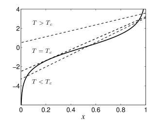
For instance, there is a single solution whenever $a\leq 0$, for which the LHS is a non–increasing function of $x$.

Next, we examine the condition for having more than one rest point, which is possible when $a>0$. Consult with Fig. 1: For sufficiently large temperature, there is only a single solution. When decreasing $T$, however, a second solution appears exactly at the point where the LHS becomes tangential to the RHS. Thus, in addition to Eq. 18, at the critical temperature we should have

$$a=\frac{1}{x(1-x)}\ ,$$ (19)

or, alternatively,

$$x=\frac{1}{2}\biggl{[}1\pm\sqrt{1-\frac{4}{a}}\biggr{]}$$ (20)

Note that the above solution exists only when $a\geq 4$. Plugging 20 into 18, we find

$$b=\ln\frac{a\pm\alpha}{a\mp\alpha}-\frac{1}{2}(a\pm\alpha)\ ,\ \alpha=\sqrt{a^{2}-4a}$$ (21)

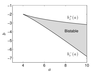
Thus, for any given $a\geq 4$, the rest point equation has three solutions whenever $b_{c}^{-}<b<b_{c}^{+}$, where

$$b_{c}^{+}=\ln\frac{a-\alpha}{a+\alpha}-\frac{a-\alpha}{2}\ ,b_{c}^{-}=\ln\frac{a+\alpha}{a-\alpha}-\frac{a+\alpha}{2}$$ (22)

For small values of $T$ when $a$ is sufficiently large (and positive), the two branches $b_{c}^{-}$ and $b_{c}^{+}$ are well separated. When one increases $T$, however, at some critical value those two branches meet and a cusp bifurcation occurs Strogatz2001 . The point where the two bifurcation curves meet can be shown to be $(a,b)=(4,-2)$, and is called a cusp point. A saddle-node bifurcation occurs all along the boundary of the region, except at the cusp point, where one has a codimension-2 bifurcation - i.e., two parameters have to be tuned for this type of bifurcation to take place Strogatz2001 . This boundary in the parameter space is shown in Fig. 2.

Figure 2: Demonstration of the cusp bifurcation in the space of parameters $a$ and $b$ for symmetric equilibria.

III.2 General Case

We now examine the most general case. We find it useful to introduce variables $u=\ln\frac{x}{1-x}$, $v=\ln\frac{y}{1-y}$. Then the interior rest point equations can be rewritten as

$$u=b+a\frac{1}{1+e^{-v}}\ ,\ v=d+c\frac{1}{1+e^{-u}}$$ (23)

where $a$, $b$ , $c$, and $d$ have been already defined in Eqs. 16, 17. Eliminating $v$ we obtain

$$\frac{1}{a}u-\frac{b}{a}=\biggl{[}1+e^{-d-\frac{c}{1+e^{-u}}}\biggr{]}^{-1}\equiv g(u)\ .$$ (24)

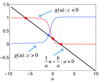
The solution of Eq. 24 are the rest point(s) of the dynamic. Its graphical representation is shown in Fig. 3.

It is easy to see that $0<g(u)<1$. Furthermore, we have from Eq. 24

$$g^{\prime}(u)=cg(1-g)\frac{1}{4\cosh^{2}\frac{u}{2}}$$ (25)

Thus, $g(u)$ is a monotonically increasing (decreasing) function whenever $c>0$ ($c<0$).

Figure 3: (Color online) Graphical representation of the general rest point equation for two different values of $c$ : Intersections represent rest points.

Next, we classify the games according to the number of rest points they allow. Let us consider two cases:

$\imath)$ $ac<0$: Note that in Eq. 24 the LHS is a monotonically increasing (decreasing) function for $a>0$ ($a<0$). As stated above, RHS is also a monotonically increasing (decreasing) function whenever $c>0$ ($c<0$). Consequently, whenever $a$ and $c$ have different signs, i.e. $ac<0$, one of the sides is a monotonically increasing function while the other is a monotonically decreasing; thus, there can be only one interior rest point, which, due to the dissipative nature of the dynamics, is globally stable. An example of this class of game is Matching Pennies that will be discussed in Section IV.

$\imath\imath)$ $ac>0$: In this case it is possible to have one, two or three interior rest points. For the sake of concreteness, we focus on $a>0$, $c>0$, so that both the LHS and RHS of Eq. 24 are monotonically increasing functions.

Recall, that at the critical point when the second solution appears, the LHS of Eq. 24 should be tangential to $g(u)$. Consider now the set of all tangential lines to $g(u)$ in Eq. 24, and let $\delta_{min}$ and $\delta_{max}$ be the minimum and maximum value of the intercepts among those tangential lines for any $u$ and $T_{Y}$. The intercept of the line given by the LHS of Eq. 24, on the other hand, equals $-\frac{b}{a}$, and is independent of the temperature. It is straightforward to check that multiple rest points are possible only when $\delta_{min}<-\frac{b}{a}<\delta_{max}$.

A full analysis along those lines (see Appendix A) reveals that the number of possible rest points depend on the ratios $\frac{b}{a}$ and $\frac{d}{c}$, as depicted in Fig. 4. First, consider the parameter range $0<-\frac{b}{a},-\frac{d}{c}<1$ (shaded light-grey region in Fig. 4), which correspond to so called coordination games that have three NE. The learning dynamics in these games can have three rest points, that intuitively correspond to the perturbed NE. In particular, those rest points will converge to the NE as the exploration rates vanish. When $a,c<0$, the parameter range $0<-\frac{b}{a},-\frac{d}{c}<1$ corresponds to so called anti-coordination games. Those games also have three NE, so the learning dynamics can have three rest points.

Let us now focus on light grey (not-shaded) regions in Fig. 4. The games in this parameter range have a single NE. At the same time, the learning dynamics might still have multiple rest points. Those additional rest-points exist only for a range of exploration rates, and disappear when both exploration rates $T_{X},T_{Y}$ are sufficiently low or sufficiently high; see Appendix B for details. An example of this type game will be presented in Section IV.

Figure 4: (Color online) Characterization of different games in the parameter space with $a,c>0$. Dark blue region corresponds to games that can have only a single rest point, whereas the games in the light grey regions can have three rest-points. The shaded grey square corresponds to games that have three Nash equilibria.

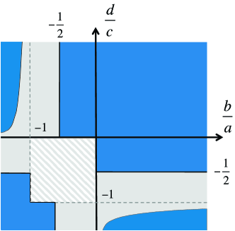
Note that the Fig. 4 was obtained by assuming that $T_{X}$ and $T_{Y}$ are independent parameters. Assuming some type of functional dependence between those two parameters alters the above characterization. For instance, consider the case $T_{X}=T_{Y}=T$. At the critical point we have (in addition to Eq. 24) $ag^{\prime}(u)=1$, which yields

$$ac=\frac{4\cosh^{2}\frac{u}{2}}{g(1-g)}$$ (26)

It can be shown that when $T_{X}=T_{Y}=T$ the above conditions can be met only when $0<-\frac{b}{a}<1$, $0<-\frac{d}{c}<1$ (shaded region in Fig. 4), which correspond to the domain of multiple NE: coordination ($a,c>0$) and anti–coordination ($a,c<0$) games.

It is illustrative to write Eq. 26 in terms of the original variables $x$ and $y$:

$$ac=\frac{1}{x(1-x)y(1-y)}$$ (27)

It can be seen that Eq. 19 is recovered when $a=c$ and $x=y$. Furthermore, since $0<x,y<1$, the above condition can be satisfied only when $ac\geq 16$.

Linear Stability Analysis

We conclude this section by briefly elaborating on the dynamic stability of the interior rest points. Note that, whenever there is a single rest point it will be globally stable due to the dissipative nature of the dynamics. Thus, we focus on the case when there are multiple rest points.

For the interior rest points, the eigenvalues of the Jacobian of the dynamical system Eqs. 14,15 are as follows:

Figure 5: (Color online) Illustration of dynamical flow for a system with three (a) and single (b) rest points. Note that the middle rest point in (a) is unstable.

$$\lambda_{1,2}=-1\pm\sqrt{acy(1-y)x(1-x)}$$ (28)

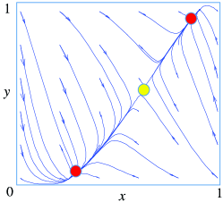
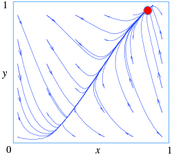
Let us focus on symmetric games and symmetric equilibria (i.e. $x=y$). From Eq. 28 we find the eigenvalues $\lambda_{1,2}=-1\pm{ax_{0}(1-x_{0})}$, so that the stability condition is $ax_{0}(1-x_{0})<1$. Recalling that at the critical point we have $a=\frac{1}{x_{0}(1-x_{0})}$, it is straightforward to demonstrate that for the middle rest–point the above condition is always violated, meaning that it is always unstable. Similar reasoning shows that two other rest points are locally stable, and depending on the starting point of the learning trajectory, the system will converge to one of the two points. An example of the flows generated by the dynamics for below–critical and above–critical exploration rates is depicted in Fig. 5 and 5.

IV Examples

We now illustrate the above findings on several games shown in Fig. 6. The row (column) number corresponds to the actions of the first (second) agent. Each cell contains a reward pair $(a_{ij},b_{ji})$, where $a_{ij}$ and $b_{ji}$ are the corresponding elements of the reward matrices $A$ and $B$.

Figure 6: Examples of reward matrices for typical two-action games.

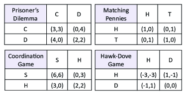
Our first example is the Prisoner’s Dilemma (PD) where each player should decide whether to Cooperate (C) or Defect (D). An example of a PD payoff matrix is shown in Fig. 6. In PD the defection is a dominant strategy – it always yields a better reward regardless of the other player choice. Thus, even though it is beneficial for the players to cooperate, the only Nash equilibrium of the game is when both players defect. For $T_{X}=T_{Y}=0$, the dynamics always converges to the NE.

In our PD example we have $\frac{b}{a}=\frac{d}{c}=-2$, so according to Fig. 4 there is a single interior rest point for any $T_{X},T_{Y}>0$. Furthermore, due to the dissipative nature of the dynamics, the system is guaranteed to converge to this rest point for any finite exploration rates. Note that this is in stark contrast from the behavior of $\epsilon$-greedy learning reported in Wunder2010 , where the authors observed that, starting from some initial conditions, the dynamics might never converge, instead alternating between different strategy regimes. The lack of convergence and chaotic behavior in their case can be attributed to the hybrid nature of the dynamics.

Next, we consider Matching Pennies (MP), which is a zero sum game where the first (second) player wins if both players select the same (different) actions; see Fig. 6. This game does not have any pure NE, but it has a mixed NE at $x^{*}=y^{*}=\frac{1}{2}$. This mixed NE is a rest point of the learning dynamics at $T_{X}=T_{Y}=0$ which is a $center$ point surrounded by periodic orbits Hofbauer1996 . For this game we have ${a}{c}<0$. Thus, there can be only one interior rest point, which can be globally stable for any $T_{X},T_{Y}>0$. Furthermore, a particular feature of this game is that finite $T_{X},T_{Y}$ does not perturb the position of the rest-point (since the entropic term is zero for $x=y=\frac{1}{2}$).

We now consider a coordination game (shaded area in Fig. 4) where players have an incentive to select the same action. In the example shown in Fig. 6, the players should decide whether to hunt a stag (S) or a hare (H). This game has two pure NE, (S,S) and (H,H), as well as a mixed NE at $(x^{*},y^{*})=(-\frac{b}{a},-\frac{d}{c})$, which, for the particular coordination game shown in Fig. 6, yields $x^{*}=y^{*}=2/5$. For sufficiently small exploration rates, the learning dynamics has three rest points that intuitively correspond to the three NE of the game. Furthermore, the rest points corresponding to the pure equilibria are stable, while the one corresponding to the mixed equilibrium is unstable.

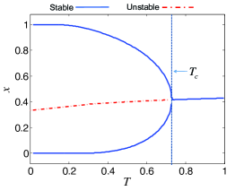
When increasing the exploration rates, there is a critical line $(T_{X}^{c},T_{Y}^{c})$ so that for any $T_{X}>T_{X}^{c},T_{Y}>T_{Y}^{c}$ only one of the rest points survives. In Fig. 7 we show the bifurcation diagram on the plane $T_{X}=T_{Y}$. We find that most coordination games are characterized by a discontinuous pitch-fork bifurcation (see Fig. 7), where above the critical line the surviving rest point correspond to the risk-dominant NE . There is an exception, however, for games with $\frac{b}{a}+\frac{d}{c}=-1$. This condition describes games where none of the pure NE are strictly risk dominant, and where the mixed NE satisfies $x^{*}+y^{*}=1$. The rest point structure undergoes a continuous pitchfork bifurcation as shown Fig. 7 whenever $a=c$ and $\frac{b}{a}+\frac{d}{c}=-1$. One can show that when the above condition is met, the critical point $u_{0}$ that satisfies $g^{\prime}(u_{0})=\frac{1}{a}$ , $\frac{1}{a}u_{0}-\frac{b}{a}=g(u_{0})$, is also the inflection point of $g(u)$, $g^{\prime\prime}(u_{0})=0$.

Figure 7: (Color online) Bifurcation diagram of the rest points for $T_{X}=T_{Y}=T$ : (a) Disconnected pitchfork, with mixed NE: $(x^{*},y^{*})=(2/5,2/5)$ (b) Continuous pitchfork, with mixed NE: $(x^{*},y^{*})=(1/3,2/3)$.

The other class of two-action games with multiple NE are so-called anti–coordination games where it is mutually beneficial for the players to select different actions. In anti–coordination games, one has $a,c<0$ whereas $0<-\frac{b}{a}<1$, $0<-\frac{d}{c}<1$. A popular example is the so called Hawk-Dove game where players should choose between an aggressive (H) or peaceful (D) behavior. This game has two pure NE, (H,D), (D,H), and a mixed NE at $(x^{*},y^{*})=(-\frac{b}{a},-\frac{d}{c})$. An example is shown in Fig. 6 with a mixed NE at $x^{*}=y^{*}=1/3$.

Anti-coordination games have similar bifurcation structure compared to the coordination games. Namely, there is a critical line $(T_{X}^{c},T_{Y}^{c})$ so that for any $T_{X}>T_{X}^{c},T_{Y}>T_{Y}^{c}$ only a single rest point survives. As in the coordination games, the bifurcation is discontinuous for most parameter values. The condition for continuous pitch-fork bifurcation in the anti-coordination games is given by $a=c$ and $\frac{b}{a}=\frac{d}{c}$. Thus, those games have a symmetric NE $x^{*}=y^{*}$. Furthrmore, the critical point where the second solution appears is also the inflection point of $g(u)$, $g^{\prime\prime}(u_{0})=0$.

Figure 8: (Color online) Bifurcation in the domain of the games with $a,c>0$, $\frac{b}{a}>0$, $-\frac{1}{2}>\frac{d}{c}>-1$. In this example we have: $\frac{d}{c}=-0.8,\frac{b}{a}=0.1$: a) Rest point structure plotted against $T_{X}$ for $T_{Y}<T_{Y}^{c}$ and $T_{Y}>T_{Y}^{c}$. b) The rest point structure plotted against $T_{Y}$ for $T_{X}^{c_{-}}<T_{X}<T_{X}^{c_{+}}(T_{Y})$. In both graphs, the red dot-dashed lines correspond to the unstable rest points.

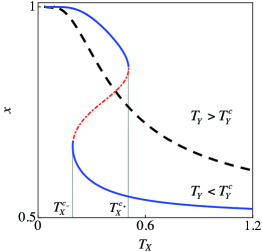
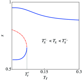
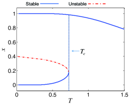
Finally, let us consider the games with a single NE, for which the learning dynamics can still have multiple rest points. To be specific, we focus on the case $a,c>0$, for which the possible regimes are outlined in Fig. 4. In Fig. 8 , we show the dependence of the rest point structure on the parameter $T_{X}$, for two different values of $T_{Y}$, for $\frac{b}{a}=0.1$, $\frac{d}{c}=-0.8$. It can be seen that for sufficiently small $T_{X}$, the learning dynamics allows a single rest point (that corresponds to the NE of the game). Similarly, there is single rest points whenever $T_{Y}$ is sufficiently hight. However, there is a critical exploration rate for agent $Y$, $T_{Y}^{c}$, so that for any $0<T_{Y}<T_{Y}^{c}$, there is a range $T_{X}^{c_{-}}(T_{Y})<T_{X}<T_{X}^{c_{+}}(T_{Y})$, for which the dynamics allows three rest points. In contrast to coordination and anti–coordination games considered above, those additional rest points do not correspond to any NE of the game. In particular, they disappear when $T_{X},T_{Y}$ are sufficiently small. We elaborate more on the appearance of those rest points in Appendix B.

Fig. 8 shows the bifurcation diagram for the same game but plotted against $T_{Y}$. Note that the two diagrams are asymmetric. In particular, in contrast to Fig. 8, here multiple solutions are possible even when $T_{Y}$ is arbitrarily small (provided that $T_{X}^{c_{-}}(T_{Y})<T_{X}<T_{X}^{c_{+}}(T_{Y})$). This asymmetry is due to the fact that the agents’ payoff matrices represent different games. In this particular case, the first player’s payoff matrix corresponds to a dominant action game, whereas the second player’s payoff matrix corresponds to a coordination game. Clearly, when $T_{X}$ is very small, the first player will mostly select the dominant action, so there can be only a single rest point at small $T_{X}$. Increasing $T_{X}$ will make the entropic term more important, until at a certain point, multiple rest points will emerge.

The same picture is preserved for the parameter range $\frac{b}{a}<-1,-\frac{1}{2}<\frac{d}{c}<0$ (the other light grey horizontal stripe). On the other hand, the players effectively exchange roles in the parameter ranges corresponding to the vertical stripes: $\frac{d}{c}>0,-1<\frac{b}{a}<-\frac{1}{2}$ and $\frac{d}{c}<-1,-\frac{1}{2}<\frac{b}{a}<0$. In this case, there is a critical exploration rate $T_{X}^{c}$, so that for any $0<T_{X}<T_{X}^{c}$, there is a range $T_{Y}^{c_{-}}(T_{X})<T_{Y}<T_{Y}^{c_{+}}(T_{X})$, for which the dynamics allows three rest points.

Finally, we note that the rest point behavior is different in the light grey regions where the parameters are also confined to $\frac{b}{a}>0,\frac{d}{c}<-1$ and $\frac{b}{a}<-1,\frac{d}{c}>0$. In those regions, multiple rest points are available only when both $T_{X}$ and $T_{Y}$ are strictly positive, i.e., $T_{X}^{c_{-}}>0$, $T_{Y}^{c_{-}}>0$.

V Discussion

We have presented a comprehensive analysis of two agent $Q$–learning dynamics with Boltzmann action selection mechanism, where the agents exploration rates are governed by temperatures $T_{X},T_{Y}$. For any two action game at finite exploration rate the dynamics is dissipative and thus guaranteed to reach a rest point asymptotically. We demonstrated that, depending on the game and the exploration rates, the rest point structure of the learning dynamics is different. When $T_{X}=T_{Y}$, for games with a single NE (either pure or mixed) there is a single globally stable rest point for any positive exploration rate. Furthermore, we analytically examined the impact of exploration/noise on the asymptotic behavior, and showed that in games with multiple NE the rest–point structure undergoes a bifurcation so that above a critical exploration rate only one globally stable solution persists. Previously, a similar observation for certain games was observed numerically in Ref. Wolpert2010 , where the authors studied Quantal Response Equilibrium (QRE) among agents with bounded rationality. In fact, it can be shown that QRE corresponds to the rest–point of the Boltzmann $Q$-learning dynamics. A similar bifurcation pictures was also demonstrated for certain continuous action games Galstyan2011JAAMAS .

In general, we observed that for $T_{X}\neq T_{Y}$, the learning dynamics is qualitatively similar for games with multiple NE. Namely, there is a bifurcation at critical exploration rates $T_{X}^{c}$ and $T_{Y}^{c}$, so that the learning dynamics allows three (single) rest points below (above) those critical values. In particular, the rest points converge to the NE of the game when $T_{X},T_{Y}\rightarrow 0$. What is perhaps more interesting is that for certain games with a single NE, it is possible to have multiple rest points in the learning dynamics when $T_{X}\neq T_{Y}$. Those additional rest points persist only for a finite range of exploration rates, and disappear when the exploration rates $T_{X}$ and $T_{Y}$ tend to zero.

We suggest that the sensitivity of the learning dynamics on exploration rate can be useful for validating various hypotheses about possible learning mechanisms in experiments. Indeed, most empirical studies so far have been limited to games with a single equilibrium, such as matching pennies, where the dynamics is rather insensitive to the exploration rate. We believe that for different games (such as coordination or anti-coordination game), the fine–grained nature of the rest point structure, and specifically, its sensitivity to the exploration rate, can provide much richer information about learning mechanisms employed by the agents.

Note Added: After completing the manuscript, we became aware of a very recent work reporting similar results Kaiser2011 , which studies convergence properties and bifurcation in the solution structure using local stability analysis. For games with a single rest point such a Prisoner’s Dilemma, local stability is subsumed by the global stability demonstrated here. The bifurcation results are similar, even though Kaiser2011 studies only coordination games and does not differentiate between continuous and discontinuous pitchfork bifurcation. Finally, the analytical form of the phase diagram Eq. 22 for the symmetric case, as well as the possibility of multiple rest points for games with a single NE demonstrated here, are complementary to the results presented in Kaiser2011 .

VI Acknowledgments

We thank Greg Ver Steeg for useful discussions. This research was supported in part by the National Science Foundation under grant No. 0916534 and the US AFOSR MURI grant No. FA9550-10-1-0569.

Appendix A Classification of games according to the number of allowable rest-points

Here we derive the conditions for multiple rest-points. We assume $a,c>0$ for the sake of concreteness.

Consider the set of all the tangential lines to $g(u)$ (see Eq. 24), and let $\delta_{T_{Y}}(u)$ be the intercept of the tangential line that passes through point $u$, $\delta_{T_{Y}}(u)=g(u)-g^{\prime}(u)u$: Here the subscript indicates that the intercept depends on the exploration rate $T_{Y}$ via coefficients $c$ and $d$. The extremum of function $\delta_{T_{Y}}(u)$ happens at $\frac{d\delta_{T_{Y}}}{du}=-g^{\prime\prime}u=0$ where:

$$g^{\prime\prime}(u)=-\frac{cg(1-g)}{16\cosh^{4}\frac{u}{2}}\biggl{(}c\tanh\biggl{[}\frac{d}{2}+\frac{c/2}{1+e^{-u}}\biggr{]}+2\sinh u\biggr{)}$$ (29)

Let $u_{0}$ be the point where $g^{\prime\prime}(u_{0})=0$. A simple analysis yields that $u_{0}>0$ whenever $d<-c/2$, and $u_{0}<0$ otherwise. Next, let $\delta_{min}=\min_{u,T_{Y}}\delta_{T_{Y}}(u)$ and $\delta_{max}=\max_{u,T_{Y}}\delta_{T_{Y}}(u)$, where minimization and maximization is over both $u$ and $T_{Y}$. It can be shown that there can be multiple solutions only when $\delta_{min}<-\frac{b}{a}<\delta_{max}$.

We now consider different possibilities depending on the ratio $\frac{d}{c}$. Due to symmetry, it is sufficient to consider $\frac{d}{c}<-\frac{1}{2}$. We differentiate the following cases:

$\imath)-1<\frac{d}{c}<-\frac{1}{2}$: In this case one has $\delta_{min}=-\infty$, $\delta_{max}=1$. Thus, there will be one rest point whenever $\frac{b}{a}<-1$.

$\imath\imath)\frac{d}{c}<-1$: In this case one has $\delta_{max}=\frac{1}{2}$, thus, there will be single rest point whenever $\frac{b}{a}<-\frac{1}{2}$. Furthermore, although an analytical expression for $\delta_{min}$ is not available, the corresponding boundary can be found by numerically solving a transcendental equation $-\frac{b}{a}=\delta_{min}$ for different $\frac{d}{c}$.

Repeating the same reasoning for $\frac{d}{c}>-\frac{1}{2}$ yields the different regions depicted in Fig. 4.

Appendix B Appearance of multiple rest points in games with single NE

We now elaborate on games with single NE for which the learning dynamics still can have multiple rest points. For the sake of concreteness, let us consider one of the regions in Fig. 4 that corresponds to $\frac{b}{a}>0$, $-1<\frac{d}{c}<-1/2$. The graphical representation of the rest point equation is shown in Fig. 9. For a given $T_{Y}$, the two lines correspond to the critical values of $T_{X}^{c_{-}}(T_{y})$ and $T_{X}^{c_{+}}(T_{Y})$. Let us consider the case $T_{Y}=0$. It is easy to see that in this limit $g(u)$ becomes a step function, $g(u)=\theta(u-{\tilde{u}})$, where ${\tilde{u}}$ is found by requiring $\frac{d}{c}+\frac{1}{1+e^{-u}}=0$, which yields $\tilde{u}=\ln\frac{-d}{d+c}$. Simple calculations yield $T_{X}^{c_{-}}(T_{Y}=0)=\frac{\tilde{a}}{\tilde{u}}\frac{b}{a}$ and $T_{X}^{c_{-}}(T_{Y}=0)=\frac{\tilde{a}}{\tilde{u}}(\frac{b}{a}+1)$, where $\tilde{a}=a_{21}+a_{12}-a_{11}-a_{22}\equiv aT_{X}$. For general $T_{Y}>0$, the corresponding values $T_{X}^{c_{-}}(T_{Y})$ and $T_{X}^{c_{+}}(T_{Y})$ can be found numerically.

Figure 9: Graphical illustration of the multi-rest point equation for a game with a single NE. Here $a,c>0$, $\frac{b}{a}=\frac{1}{2}$, $\frac{d}{c}=-\frac{3}{4}$.

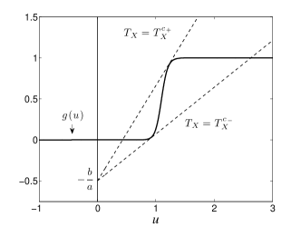
Finally, note that when increasing $T_{Y}$, there is a critical exploration rate $T_{Y}=T_{Y}^{c}$ so that for $T_{Y}>T_{Y}^{c}$ the multiple solutions will disappear. It is easy to see that $T_{Y}^{c}$ corresponds to the point when the maximum value of the intercept to $g(u)$ for a given $T_{Y}$ equals $-\frac{b}{a}$.

References

- (1) R.S. Sutton and A.G. Barto. Reinforcement learning: An introduction. The MIT press, 2000.
- (2) C. Claus and C. Boutilier. The dynamics of reinforcement learning in cooperative multiagent systems. In Proc. of AAAI-1998/IAAI -1998, 1998.
- (3) S. Singh, M. Kearns, and Y. Mansour. Nash convergence of gradient dynamics in general-sum games. In Proc. of Uncertainty in AI-2000, 2000.
- (4) M. Bowling and M. Veloso. Rational and convergent learning in stochastic games. In Proc. of IJCAI, 2001.
- (5) J. Hofbauer and K. Sigmund. Evolutionary games and Population dynamics. Cambridge University Press, 1998.
- (6) Y. Sato and J.P. Crutchfield. Coupled replicator equations for the dynamics of learning in multiagent systems. Physical Review E, 67(1), 2003.
- (7) Y. Sato, E. Akiyama, and J.P. Crutchfield. Stability and diversity in collective adaptation. Physica D: Nonlinear Phenomena, 210(1-2):21 – 57, 2005.
- (8) K. Tuyls, K. Verbeeck, and T. Lenaerts. A selection-mutation model for -learning in multi-agent systems. In proc. of AAMAS-2003, pages 693–700, 2003.
- (9) E. Gomes and R. Kowalczyk. Dynamic analysis of multiagent -learning with -greedy exploration. In Proc. of ICML-2009, 2009.
- (10) M. Wunder, M. Littman, and M. Babes. Classes of multiagent -learning dynamics with -greedy exploration. In Proc. of ICML-2010, 2010.
- (11) D. Lee, M.L. Conroy, B.P. McGreevy, and D.J. Barraclough. Reinforcement learning and decision making in monkeys during a competitive game. Cognitive Brain Research, 22(1):45–58, 2004.
- (12) S. Kim, J. Hwang, H. Seo, and D. Lee. Valuation of uncertain and delayed rewards in primate prefrontal cortex. Neural Networks, 22(3):294–304, 2009.
- (13) C.J. Burke, P.N. Tobler, M. Baddeley, and W. Schultz. Neural mechanisms of observational learning. PNAS, 107(32):14431, 2010.
- (14) K. Tuyls, P.J.T. Hoen, and B. Vanschoenwinkel. An evolutionary dynamical analysis of multi-agent learning. JAAMAS, 12(1):115–153, 2006.
- (15) E. Hopkins. Two Competing Models of How People Learn in Games. Econometrica, 70(6):2141–2166, 2002.
- (16) J. Hofbauer and E. Hopkins. Learning in perturbed asymmetric games. Games and Economic Behavior, 52(1):133–152, 2005.
- (17) C.J.C.H. Watkins and P. Dayan. Technical note: -learning. Machine learning, 8(3):279–292, 1992.
- (18) D.S. Leslie and E.J. Collins. Individual -learning in normal form games. SIAM Journal on Control and Optimization, 44(2):495–514, 2006.
- (19) K. Friston. The free-energy principle: a unified brain theory? Nature Reviews Neuroscience, 11(2):127–138, 2010.
- (20) J. Hofbauer and K. Sigmund. Evolutionary game dynamics. Bulletin of the American Mathematical Society, 40(4):479, 2003.
- (21) J. Hofbauer. Evolutionary dynamics for bimatrix games: A hamiltonian system? Journal of Mathematical Biology, 34:675–688, 1996.
- (22) T. Borgers and R. Sarin. Learning through reinforcement and replicator dynamics,. Journal of Economic Theory, 77(1):1 – 14, 1997.
- (23) Y. Sato, E. Akiyama, and J. D. Farmer. Chaos in learning a simple two-person game. PNAS, 99(7):4748–4751, 2002.
- (24) Tobias Galla. Intrinsic noise in game dynamical learning. Phys. Rev. Lett., 103:198702, Nov 2009.
- (25) S. H. Strogatz. Nonlinear Dynamics And Chaos. Westview Press, 2001.
- (26) Wolpert D.H., M. Harre, Olbrich E., Bertschinger N., and Jost J. Hysteresis effects of changing the parameters of noncooperative games. to be published in Phys. Rev. E, also Arxiv preprint arXiv:1010.5749, 2010.
- (27) Aram Galstyan. Continuous strategy replicator dynamics for multi–agent learning. to be published in JAAMAS, 2011.
- (28) M. Kaiser and K. Tuyls. Faq-learning in matrix games: Demonstrating convergence near nash equilibria, and bifurcation of attractors in the battle of sexes. AAAI IDGT’11 workshop, August 2011.