Non-existence of invariant EPR correlation for two qu$\boldsymbol{d}$its, $\boldsymbol{d}>2$

Abstract

The two qubit (spin $1/2$) singlet state has invariant perfect EPR correlations: if two observers measure any identical observables the results are always perfectly (anti-)correlated. We show that no such correlations exists in $d\otimes d$ pure or mixed bipartite quantum states if $d\geq 3$. This points that two qubit singlets are high-quality quantum information carriers in long distance transmission: their correlations are unaffected by identical random unitary transformations of both qubits. Pairs of entangled qu$d$its, $d>2$, do not have this property. Thus, qu$d$it properties should be rather exploited only in protocols in which transmission is not a long distance one.

The power of entanglement comes from the correlations. Properties of correlations of a maximally entangled state are purely quantum, without any classical analog. Recent research dedicated to the nature of entanglement and quantum correlations is in diverse directions: e.g., the relation between quantum correlation and classical correlation correlation0 ; correlation1 ; correlation2 ; correlation3 ; correlation4 ; correlation-1 , quantification of quantum correlations discord1 ; correlation4 ; discord2 ; discord3 ; discord4 ; discord5 ; discord6 , quantum communication complexity complexity ; quantsim4 .

We shall analyze invariance properties of quantum correlations. A two qubit singlet has the following property. Imagine two observes, Alice and Bob, who make measurements on their qubits. Irrespective of the actual measurement setting they both use, provided they measure two identical observables, the results are always perfectly (anti-)correlated. We shall call such a property invariant perfect correlation. It has been used in the Ekert 1991 entanglement based quantum cryptography protocol EKERT , and is important in many quantum communication schemes. The Bloch Sphere representation of qubit observables allows one to put them as $\vec{\gamma}^{X}\cdot\vec{\sigma}^{X}$, where $\vec{\gamma}^{X}$ is a unit real three dimensional vector, and $\vec{\sigma}^{X}$ is a vector composed of Pauli spin operators, and $X=A,B$ denotes the observers. If Alice and Bob use identical measurement settings for their devices we have $\vec{\gamma}^{A}=\vec{\gamma}^{B}$, and their results fulfill $r_{A}=-r_{B}$, where $r_{X}=\pm 1$.

Do we have a similar property for higher dimensional systems, including higher dimensional singlets? The general answer, which we give here, is no. One might be surprised that this negative result holds also for singlets, as results of measurements on higher dimensional singlets are invariantly correlated in the case of spin observables. However, such observables form only a subset of all possible ones. Correlations for other observables, e.g. ZZH , behave differently .

This has important ramifications. There is a tendency to investigate properties of entangled qu$d$its in the hope of getting better realizations of quantum communication protocols GISIN . Such protocols usually comprise of transfer of the (entangled) objects, manipulations and finally measurements. Upon a long distance transfer entangled systems face disturbances. One of them is decoherence, which we shall not discuss here. However, even if decoherence is avoided, systems may suffer from random unitary transformations, due to imperfections of the transmission. The most known are random polarization transformations of polarization qubits in optical fibers. One of the remedies is to pass both entangled qubits in a singlet state (almost) simultaneously via the same transmission line charlie , as it was suggested and experimentally tested by Banaszek et al. BANASZEK . The singlet is invariant with respect to of $U\otimes U$ transformations. This is equivalent to the property of possessing an invariant perfect correlation discussed above. Thus its correlations are intact to such a disturbance of the transmission lines. Is there a similar solution possible for qu$d$its ($d>2$)? Our results point to a negative answer. There is no two qu$d$it entangled state, pure or mixed which, has EPR-type correlations invariant with respect to random, but identical, unitary transformations applied to both subsystems. This suggests that the qu$d$it properties should be rather exploited only in quantum information protocols in which transmission is not a long distance one. The invariant correlations of two qubit singlets, single them out to be best for applications requiring long distance transfer of quantum information.

In order to substantiate the above claims, let us start with an analysis of invariant perfect correlations in two qubit states. If the measurement basis is arbitrary but identical for both subsystems, the measurement results on the two subsystems are deterministically EPR correlated and the correlation type is invariant with respect to identical changes of the measurement basis on both sides of the experiment. With respect to spin measurements, represented by Pauli operators, intuitively, there may exist two types of invariant correlations in two-qubit states: type I: $\pm 1\leftrightarrow\pm 1$, and type II: $\pm 1\leftrightarrow\mp 1$ where $\leftrightarrow$ denotes the correspondence between the measurement outputs of the two subsystems. The following theorem is known to hold for pure states, we present a version for arbitrary states.

Theorem 1. In a $2\otimes 2$ composite Hilbert space, the correlation of type I exists only in the singlet state $|\psi^{-}\rangle=\frac{1}{\sqrt{2}}(|0^{A}\rangle|1^{B}\rangle-|1^{A}\rangle_{A}|0^{B}\rangle),$ and the correlation of type II does not exist in any pure or mixed state.

Proof. The density operator of an arbitrary $2\otimes 2$ bipartite state can be generally written as

$$\rho^{AB}= \frac{1}{4}[I^{A}\otimes I^{B}+(\boldsymbol{\alpha}\cdot\boldsymbol{\sigma}^{A})\otimes I^{B}+I^{A}\otimes(\boldsymbol{\beta}\cdot\boldsymbol{\sigma}^{B})$$ (1)

$$+\sum_{i,j=1}^{3}T_{ij}\sigma_{i}^{A}\otimes\sigma_{j}^{B}].$$

The vectors $\boldsymbol{\alpha}$, $\boldsymbol{\beta}$ and components $T_{ij}$, $i=1,\,2,\,3$, which form the correlation tensor $T$, are real. One has $||\boldsymbol{\alpha}||\leq 1,\,||\boldsymbol{\beta}||\leq 1,$ $|T_{ij}|\leq 1$, and $||\boldsymbol{\alpha}||^{2}+||\boldsymbol{\beta}||^{2}+||T||^{2}\leq 3$

If for all $\vec{n}$ the state $\rho_{AB}$ satisfies $\langle\boldsymbol{n}\cdot\boldsymbol{\sigma}^{A}\otimes\boldsymbol{n}\cdot\boldsymbol{\sigma}^{B}\rangle=-1,$ then the correlation of type I, and if the right hand side is $1$, the type is II.

By straightforward calculation, we can get the following property of the correlation function $\langle\boldsymbol{n}\cdot\boldsymbol{\sigma}^{A}\otimes\boldsymbol{n}\cdot\boldsymbol{\sigma}^{B}\rangle=\boldsymbol{n}{T}\boldsymbol{n}^{\mathrm{T}},$ where ${T}$ is a $3\times 3$ matrix with the components of the correlation tensor $T_{ij}$ as its $ij$-th elements. The symbol $(\cdot)^{\mathrm{T}}$ denotes the transposition of a column vector.

If $\langle\boldsymbol{n}\cdot\boldsymbol{\sigma}^{A}\otimes\boldsymbol{n}\cdot\boldsymbol{\sigma}^{B}\rangle=\pm 1$ and the same sign applies to all $\boldsymbol{n}$, one can easily show that that ${T}=\pm{I}_{3}+{X},$ where ${I}_{3}$ is the identity matrix of order $3$ and $X$ is a real anti-symmetric matrix. Thus

$$\rho^{AB}= \frac{1}{4}[I^{A}\otimes I^{B}\pm\sum_{i=1}^{3}\sigma_{i}^{A}\otimes\sigma_{i}^{B}$$ (2)

$$+\sum_{1\leq i<j\leq 3}X_{ij}(\sigma_{i}^{A}\otimes\sigma_{j}^{B}-\sigma_{j}^{A}\otimes\sigma_{i}^{B})$$

$$+(\boldsymbol{\alpha}\cdot\boldsymbol{\sigma}^{A})\otimes I^{B}+I^{A}\otimes(\boldsymbol{\beta}\cdot\boldsymbol{\sigma}^{B})].$$

Suppose the eigenvalues of $\rho_{AB}$ in Eq. (2) are $\lambda_{1}$, $\lambda_{2}$, $\lambda_{3}$, $\lambda_{4}$, then these four eigenvalues are the roots of the equation $\mathrm{Det}(\lambda I^{A}\otimes I^{B}-\rho^{AB})=0.\$ By Vieta’s Theorem Vieta , we have

$$\sum_{1\leq i<j\leq 4}\lambda_{i}\lambda_{j}=-\frac{1}{8}(||\boldsymbol{\alpha}||^{2}+||\boldsymbol{\beta}||^{2}+||X||^{2})\leq 0.$$ (3)

for both “$\pm$” in Eq. (2), where $||X||^{2}=\mathrm{Tr}(X^{\dagger}X)$.

According to $\rho^{AB}\geq 0$, i.e., $0\leq\lambda_{1},\,\lambda_{2},\,\lambda_{3},\,\lambda_{4}\leq 1$, it can be inferred from (3) that $\boldsymbol{\alpha}=\boldsymbol{\beta}=\boldsymbol{0}$, $X=0$, so $\rho^{AB}$ is simplified to

$$\rho^{AB}=\frac{1}{4}(I^{A}\otimes I^{B}\pm\sum_{i=1}^{3}\sigma_{i}^{A}\otimes\sigma_{i}^{B}).$$ (4)

When $\langle\boldsymbol{n}\cdot\boldsymbol{\sigma}^{A}\otimes\boldsymbol{n}\cdot\boldsymbol{\sigma}^{B}\rangle=+1$ for all $\boldsymbol{n}\in\mathbb{R}^{3}$, Eq. (4) should take “$+$”, but it can be shown that in this case the eigenvalues of $\rho^{AB}$ are $\pm\frac{1}{2}$, each with multiplicity $2$, so $\rho^{AB}$ is not positive, and thus no bipartite quantum state satisfies $\langle\boldsymbol{n}\cdot\boldsymbol{\sigma}^{A}\otimes\boldsymbol{n}\cdot\boldsymbol{\sigma}^{B}\rangle=+1$ for all $\boldsymbol{n}\in\mathbb{R}^{3}$.

When $\langle\boldsymbol{n}\cdot\boldsymbol{\sigma}^{A}\otimes\boldsymbol{n}\cdot\boldsymbol{\sigma}^{B}\rangle=-1$ for all $\boldsymbol{n}\in\mathbb{R}^{3}$, Eq. (4) should take “$-$”, and it can be shown that in this case the eigenvalues of $\rho^{AB}$ are $1$ and $0$ (with multiplicity $3$), satisfying $\rho^{AB}\geq 0$, and it is a pure quantum state. By simple calculation, it can be verified that $\rho^{AB}=|\psi^{-}\rangle\langle\psi^{-}|$, exactly the singlet state. $\blacksquare$

Theorem 1 is independent of the assumed definition of operators used in the reasoning. One could claim that type II correlations are possible, as in a way Bob could interpret his observables as $-\vec{\gamma}_{B}\cdot\vec{\sigma}_{B}$. But this would lead to inconsistency between operator algebras of A and B, as $(-\vec{x}\cdot\vec{\sigma})(-\vec{y}\cdot\vec{\sigma})\neq-i\vec{z}\cdot\vec{\sigma}$. Thus the reached result is objective. This is why a state with permuted basis states of one of the observers, $\frac{1}{\sqrt{2}}(|0^{A}\rangle|0^{B}\rangle-|1^{A}\rangle_{A}|1^{B}\rangle)$, does not have invariant perfect correlations.

Do similar correlations like type I or II exists in bipartite quantum systems of higher dimensions?

We define a general invariant perfect correlation for two qu$d$it states as follows: if two measurements along the same arbitrary orthogonal basis $\{|m_{1}\rangle,\cdots,|m_{d}\rangle\}$ are performed on both subsystems, the outputs of the two measurements are deterministically correlated as a one-to-one map, and the map is invariant with respect to changes of the measurement basis. Different one-to-one maps between the outputs at the two sides provide a classification of different types of perfect correlations. Note that, this definition requires that invariant perfect correlation must be independent of the labeling (or, ordering) of the measurement basis states.

Directed graphs, e.g. Fig. 1 and 2, classify the different types of perfect correlations that may exist in two qu$d$it states. The states of the measurement basis are represented by vertices. If two measurement results are correlated, the corresponding vertices are connected by a directed edge. All directed edges start from the same subsystem (e.g., $A$) and end at the other one. In other words, each vertex has double “identity”: if it is the starting vertex of an edge, it denotes a measurement result of subsystem $A$ and otherwise it denotes a measurement result of subsystem $B$. Such graphical representation will not cause any confusion or ambiguity because the edges are directed and the projective measurements on the two subsystems are along the same basis. The advantage of such a graphical way to characterize different types of perfect correlations is that a directed graph defined above stays essentially invariant under different labeling of the vertices,that is, a perfect correlation is unchanged under a re-ordering of the states of a measurement basis, so one possible perfect correlation corresponds to one such directed graph.

Fig. 1 shows all possible types of perfect correlations that may exist in $2\otimes 2$ bipartite quantum states, and Fig. 2 shows all possible types of perfect correlations that may exist in $3\otimes 3$ bipartite quantum states. It is evident that there can be only two structures in a directed graph representing perfect correlation: loops (i.e. a directed edge starts from and ends at the same vertex) or circles.

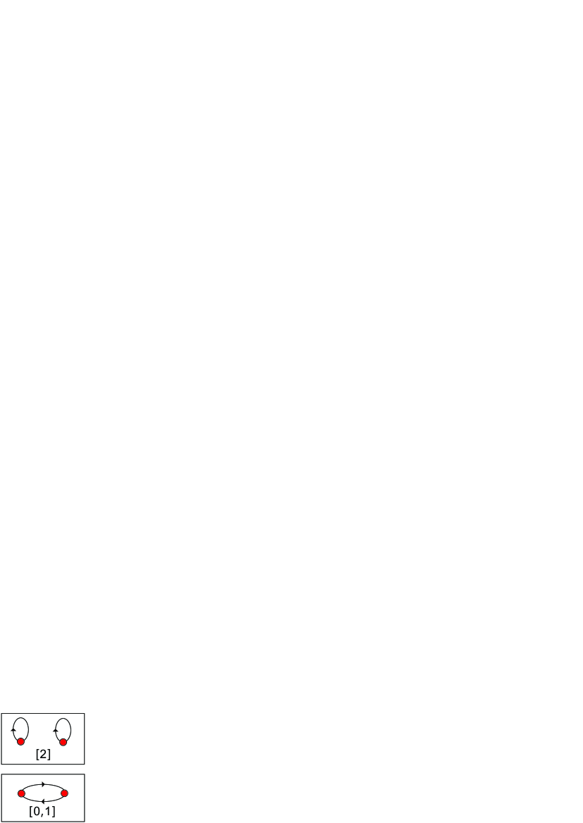
Figure 1: Possible types of perfect correlations that may exist in $2\otimes 2$ bipartite quantum states.

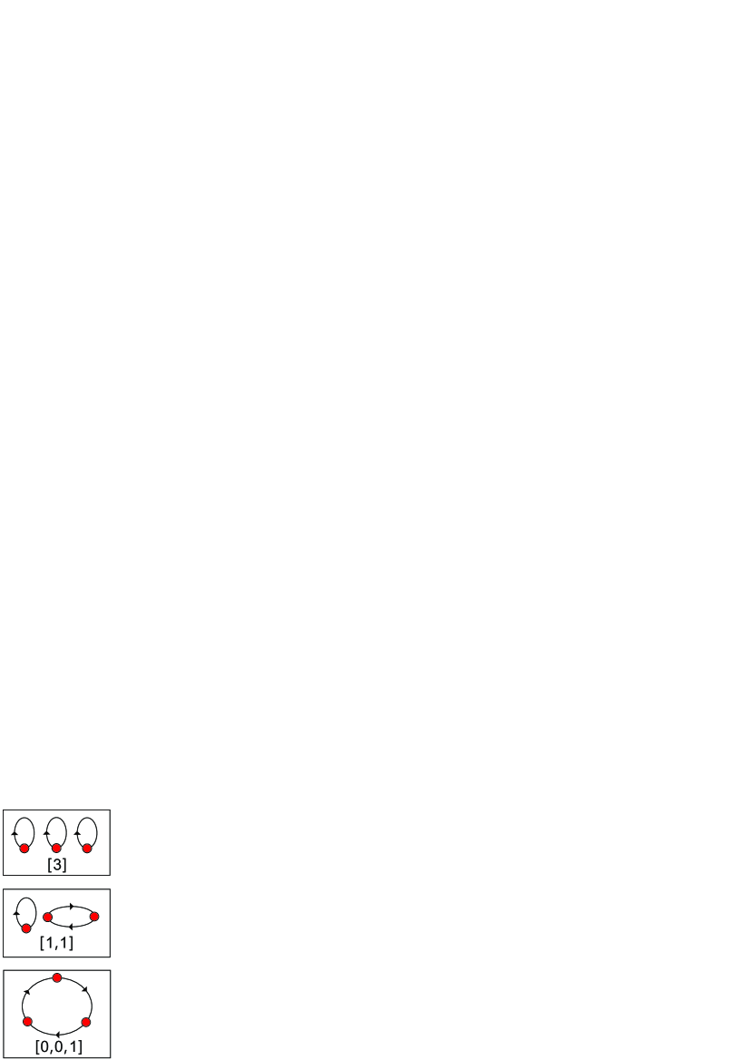
Figure 2: Possible types of perfect correlations that may exist in $3\otimes 3$ bipartite quantum states

We use a short-hand notation $[n_{1},n_{2},\cdots,n_{w}]$ to denote the graph with $n_{1}$ loops, $n_{2}$ circles of two vertices, $\cdots$, $n_{w}$ circles of $w$ vertices, and $w$ is the number of vertices in the largest circle of the graph. For instance, $[0,1]$ and $[2]$ denote the correlations in type I and type II respectively; and $[d]$ denotes the perfect correlation that measurements on both subsystems along the same basis always yield the same outcome.

Basing on the above definition of perfect correlation, we set out to study whether perfect correlation exists in higher dimensional pure or mixed bipartite quantum states. We find that when $d\geq 3$ no $d\otimes d$ bipartite quantum state, whether pure or mixed, has any type of invariant perfect correlations at all, thus the two-qubit singlet $|\psi^{-}\rangle$ is the unique state possessing an invariant perfect correlation.

We first present a lemma.

Lemma 1. If $d\geq 3$, perfect correlations other than $[d]$ cannot exist for any two qu$d$it quantum states.

Proof. Suppose there exists a $d\otimes d$ bipartite state $\rho^{AB}$ which has perfect correlation other than $[d]$. For projective measurements, on the two subsystems , along the same orthogonal basis $\{|e_{1}\rangle,|e_{2}\rangle,\cdots,|e_{d}\rangle\}$ one has

$$\langle e_{1}^{A}|\rho^{AB}|e_{1}^{A}\rangle=c|e_{p}^{B}\rangle\langle e_{p}^{B}|,\,p\neq 1\,c>0.$$ (5)

However, we can change the basis with respect to which the state is defined, to another orthogonal basis $\{|e_{1}\rangle,|e_{2}^{\prime}\rangle,\cdots,|e_{d}^{\prime}\rangle\}$ which has only one state $|e_{1}\rangle$ in common with the first basis $\{|e_{1}\rangle,|e_{2}\rangle,\cdots,|e_{d}\rangle\}$, i.e., $|e_{i}\rangle\langle e_{i}|\neq|e_{j}^{\prime}\rangle\langle e_{j}^{\prime}|$, $\forall i,j=2,\cdots,d$. Then, according to the definition of perfect correlation,

$$\langle e_{1}^{A}|\rho^{AB}|e_{1}^{A}\rangle=c^{\prime}|e_{q}^{\prime B}\rangle\langle e_{q}^{\prime B}|,\,q\neq 1\,c^{\prime}>0,$$ (6)

but $|e_{p}^{B}\rangle\neq|e_{q}^{\prime B}\rangle$, so Eq. (6) contradicts Eq. (5). Thus, perfect correlations other than $[d]$ cannot exist in $d\otimes d$ ($d\geq 3$) systems. $\blacksquare$

Note that the type of basis change used in the proof is possible only for $d>2$. This is why the perfect correlation $[0,1]$ exists for the $2\otimes 2$ state $|\psi^{-}\rangle$.

Note that, Lemma 1 does not guarantee that perfect correlation of identity maps does exist in some $d\otimes d$ ($d\geq 3$) quantum states. Actually we have the following.

Theorem 2. When $d\geq 3$, no $d\otimes d$ pure or mixed bipartite states has any type of perfect correlations.

Proof for the pure states. According to Lemma 1, we only need to consider the perfect correlation $[d]$. Assume that a $d\otimes d$ state $|\Phi\rangle$ has such a correlation. Thus, for an arbitrary basis $\{|e_{1}\rangle,\cdots,|e_{d}\rangle\},$ $|\Phi\rangle$ should have the following form:

$$|\Phi\rangle=\alpha_{1}|e_{1}\rangle|e_{1}\rangle+\cdots+\alpha_{d}|e_{d}\rangle|e_{d}\rangle,\;\alpha_{1},\cdots,\alpha_{d}\in\mathbb{C}.$$ (7)

Let us change the measurement basis to $\{|f_{1}\rangle,|f_{2}\rangle,\cdots,|f_{d}\rangle\}$ such that $\{|f_{1}\rangle,\,|f_{2}\rangle\}$ spans the same subspace spanned by $\{|e_{1}\rangle,|e_{2}\rangle\}$. The invariant perfect correlation $[d]$ for $|\Phi\rangle$, implies that if the measurement in the new basis on one of the subsystems produces an output linked with$|f_{1}\rangle$ or $|f_{2}\rangle$, the second measurement will produce an identical output. Thus, the two-dimensional (unnormalized) state

$$|\phi\rangle=\alpha_{1}|e_{1}\rangle|e_{1}\rangle+\alpha_{2}|e_{2}\rangle|e_{2}\rangle$$ (8)

has perfect correlation $[2]$, i.e. type II, which is a contradiction with the property of $|\psi^{-}\rangle$. $\blacksquare$

Proof for mixed states. Again, Lemma 1 tells that a mixed bipartite quantum state $\rho_{AB}$ can have an invariant perfect correlation only of type $[d]$. For measurements on the two subsystems of $\rho_{AB}$ are along the same basis, e.g. $\{|e_{1}\rangle,\cdots,|e_{d}\rangle\}$, we have

$$\mathrm{Prob}(i,j)=\langle e_{i}^{A}|\langle e_{j}^{B}|\rho^{AB}|e_{i}^{A}\rangle|e_{j}^{B}\rangle=0,\quad\forall i\neq j.$$ (9)

Thus, the eigenstates of $\rho^{AB}$ lie in the subspace spanned by $\{|e_{i}^{A}\rangle|e_{i}^{B}\rangle$, $i=1,\cdots,d\}$. Suppose the rank of $\rho_{AB}$ is $r$, and let

$$|g_{k}^{AB}\rangle=\sum_{i}\gamma_{k,i}|e_{i}^{A}\rangle|e_{i}^{B}\rangle,\;k=1,\cdots,r,$$ (10)

be the eigenstates of $\rho_{AB}$, then

$$\rho^{AB}=\sum_{k=1}^{r}\lambda_{k}|g_{k}^{AB}\rangle\langle g_{k}^{AB}|.$$ (11)

Thus, $\rho_{AB}$ must have the form

$$\rho_{AB}=\sum_{i,j=1}^{d}\alpha_{i,j}|e_{i}^{A}\rangle|e_{i}^{B}\rangle\langle e_{j}^{A}|\langle e_{j}^{B}|,$$ (12)

where $\alpha_{i,j}=\sum_{k}\lambda_{k}\gamma_{k,i}\gamma_{k,j}^{*}$.

Let us take an arbitrary orthogonal basis as the measurement basis on both subsystems. We choose a state of the basis $|m\rangle=\sum_{k=1}^{d}m_{i}|e_{k}\rangle.$ The invariant perfect correlation $[d]$ implies that if the measurement on the subsystem $A$ produces the output linked with $|m^{A}\rangle$, the state of the subsystem $B$ collapses to $|m^{B}\rangle$. Therefore,

$$\langle m^{A}|\rho^{AB}|m^{A}\rangle =\sum_{i,j,k,l=1}^{d}m_{k}^{*}m_{l}\alpha_{i,j}\delta_{i,k}\delta_{j,l}|e_{i}^{B}\rangle\langle e_{j}^{B}|$$ (13)

$$=\sum_{i,j=1}^{d}m_{i}^{*}m_{j}\alpha_{i,j}|e_{i}^{B}\rangle\langle e_{j}^{B}|=c_{|m\rangle}|m^{B}\rangle\langle m^{B}|$$

$$=c_{|m\rangle}\sum_{i,j=1}^{d}m_{i}^{*}m_{j}|e_{i}^{B}\rangle\langle e_{j}^{B}|,$$

where $c_{|m\rangle}$ is the probability that the measurement produces the output $|m\rangle$. Since Eq. (13) should hold true for arbitrary $|m\rangle$, we have $\alpha_{i,j}=c_{|m\rangle}.$ Therefore,

$$\rho_{AB} =c_{|m\rangle}\sum_{i,j=1}^{d}|e_{i}^{A}\rangle|e_{i}^{B}\rangle\langle e_{j}^{A}|\langle e_{j}^{B}|$$ (14)

$$=c_{|m\rangle}(\sum_{i=1}^{d}|e_{i}^{A}\rangle|e_{i}^{B}\rangle)(\sum_{j=1}^{d}\langle e_{j}^{A}|\langle e_{j}^{B}|).$$

Thus, $\rho_{AB}$ is a pure bipartite quantum state, contradicting the assumption that $\rho_{AB}$ is a mixed state. $\blacksquare$

Combining Theorem 1 and 2, we finally reach:

Theorem 3. Among all $d\otimes d$ ($d\geq 2$) bipartite quantum states, pure or mixed, only the two-qubit singlet state has an invariant perfect correlation (it is of type $[0,1]$).

Thus our claim is substantiated. Note that, Theorem 3 does not state that there are no EPR correlations in bipartite states other than $|\psi^{-}\rangle$. Our results consider only the invariance property of the correlations. Such studies could be extended to multi-qu$d$it systems. We conjecture that this would single out various types of multiqubit singlets CABELLO as possessing invariant correlations. It is worth noting that such singlets are already within experimental reach, see MOHAMED .

Supported by the NNSF of China (Grant 11075148), the Fundamental Research Funds for the Central Universities, the CAS and the National Fundamental Research Program. SP also acknowledges the Innovation Foundation of USTC. MZ acknowledges VII UE FP project Q-ESSENCE, and a MNiSW grant N202 208538.

References

- (1) R. Horodecki et al. Rev. Mod. Phys.81 , 865 (2009)
- (2) B. Groisman, S. Popescu and A. Winter, Phys. Rev. A 72, 032317 (2005).
- (3) D. Kaszlikowski et al. Phys. Rev. Lett. 101, 070502 (2008).
- (4) K. Modi et al. Phys. Rev. Lett. 104, 080501 (2010).
- (5) G. Adesso and A. Datta, Phys. Rev. Lett. 105, 030501 (2010).
- (6) L. Henderson and V. Vedral, J. Phys. A: Math. Gen. 34 6899 (2001).
- (7) H. Ollivier and W. H. Zurek, Phys. Rev. Lett. 88, 017901 (2001).
- (8) J. Oppenheim et al. Phys. Rev. Lett. 89, 180402 (2002).
- (9) S. Luo, Phys. Rev. A 77, 022301 (2008).
- (10) S. Luo and S. Fu, Phys. Rev. A 82, 034302 (2010).
- (11) P. Giorda and M. G. A. Paris, Phys. Rev. Lett. 105, 020503 (2010).
- (12) Z. -Y. Sun et al. Phys. Rev. A 82, 032310 (2010).
- (13) D. Bacon and B. F. Toner, Phys. Rev. Lett. 90, 157904 (2003).
- (14) H. Buhrman et al. Rev. Mod. Phys. 82, 665 (2010).
- (15) A. Ekert, Phys. Rev. Lett. 67, 661 (1991).
- (16) Żukowski, M., A. Zeilinger, and M.A. Horne, Phys. Rev. A 55, 2464 (1997).
- (17) C. Brukner, M. Żukowski , and A. Zeilinger, Phys. Rev. Lett. 89, 197901 (2002) T. Durt et al. Phys. Rev. A 67, 012311(2003);
- (18) For other direct benefits of such a scheme see the following. Suppose Charlie is a quantum resource provider who sells correlated pairs to other people. If the correlation is not invariant, then Charlie has to tell the buyers the directions along which they can get the perfect EPR correlations. But information on the directions requires an infinite number bits to be encoded precisely, and this has to be passed to the buyers. If the correlation is invariant, such a problem can be avoided.
- (19) K. Banaszek et al. Phys. Rev. Lett. 92, 257901 (2004)
- (20) Vieta’s theorem characterizes the relation between the coefficients and the roots of a polynomial equation as follows: suppose is a polynomial equation defined on the complex field and it has roots denoted by , then there must be .
- (21) A. Cabello, Phys. Rev. A 75, 020301(R) (2007).
- (22) M. Eibl et al. Phys. Rev. Lett. 90, 200403 (2003); M. Radmark, M. Żukowski, and M. Bourennane, Phys. Rev. Lett. 103, 150501 (2009)