Entanglement study of the 1D Ising model with Added Dzyaloshinsky-Moriya interaction

Abstract

We have studied occurrence of quantum phase transition in the one-dimensional spin-1/2 Ising model with added Dzyaloshinsky-Moriya (DM) interaction from bi-partite and multi-partite entanglement point of view. Using exact numerical solutions, we are able to study such systems up to $24$ qubits. The minimum of the entanglement ratio $R\equiv\tau_{2}/\tau_{1}<1$, as a novel estimator of QPT, has been used to detect QPT and our calculations have shown that its minimum took place at the critical point. We have also shown both the global-entanglement (GE) and multipartite entanglement (ME) are maximal at the critical point for the Ising chain with added DM interaction. Using matrix product state approach, we have calculated the tangle and concurrence of the model and it is able to capture and confirm our numerical experiment result. Lack of inversion symmetry in the presence of DM interaction stimulated us to study entanglement of three qubits in symmetric and antisymmetric way which brings some surprising results.

1 INTRODUCTION

In the last few years it has become apparent that quantum information may lead to further insight into other areas of physics such as condensed matter and statistical mechanics [1, 2, 3, 4, 5, 6, 7, 8, 9, 10, 11, 12]. The attention of the quantum information community to study in condensed matter has stimulated an exciting cross fertilization between the two areas. It has been found that entanglement plays a crucial role in the low-temperature physics of many of these systems, particularly in their ground state[4, 5, 6, 7, 10]. Quantum phase transition (QPT) happens at zero temperature and shown non analyticity in the physical properties of the ground state by the change of a parameter $\lambda$ of the Hamiltonian $H(\lambda)$. This change is driven only by quantum fluctuations[13]. Since QPT occurs at $T=0$, the emerging correlations have a purely quantum origin. Therefore, it is reasonable to conjecture that entanglement is a crucial ingredient for the occurrence of the QPT [4, 6, 7, 14, 15, 16]. Wu et al. [7] have shown that a discontinuity in a bipartite entanglement measure (concurrence[15] and negativity [16]) is a necessary and sufficient indicator of a first-order quantum phase transition, negativity being characterized by a discontinuity in the first derivative of the ground state energy. They have also shown that a discontinuity or a divergence in the first derivative of the same measure (assuming it is continuous) is a necessary and sufficient indicator of a second-order QPT, that is characterized by a discontinuity or a divergence of the second derivative of the ground state energy.

Dzyaloshinsky has shwon[17] that, in crystal with no inversion center, the usual isotropic exchange $J\vec{S}_{i}.\vec{S}_{j}$ is not the only magnetic interaction and antisymmetric exchange $\vec{D}_{ij}.(\vec{S}_{i}\times\vec{S}_{j})$ is allowed. Later, Moriya has shown[18]that inclusion of spin orbit coupling on magnetic ions in 1st and 2nd order leads to antisymmetric and anisotropic exchange respectively. This interaction is, however, rather difficult to handle analytically, but it is one of the agents responsible for magnetic frustration. Since this interaction may induce spiral spin arrangements in the ground state[19], it is closely involved with ferroelectricity in multiferroic spin chains[20, 21]. Besides, the DM interaction plays an important role in explaining the electron spin resonance experiments in some one-dimensional antiferromagnets[22]. Moreover, the DM interaction modifies the dynamic properties[23] and quantum entanglement[24] of spin chains[25]. In the present paper, we are interested to study the one-dimensional spin-1/2 Ising model with added DM interaction from quantum entanglement point of view using variational matrix product state and numerical exact diagonalization methods. The Hamiltonian is given by

$$\emph{H}=J\sum_{j=1}^{N}S_{j}^{z}S_{j+1}^{z}+\sum_{j=1}^{N}\vec{D}.\left(\vec{S}_{j}\times\vec{S}_{j+1}\right),$$ (1)

where $\overrightarrow{S}_{j}$ is spin-$1/2$ operator on the $j$-th site, and $J>0$ $(J<0)$ denotes antiferromagnetic (ferromagnetic) coupling constant. In very recent works[26, 27] respectively studied the ground state phase diagram of the ferromagnetic and antiferromagnetic Ising chain in the presence of the uniform DM interaction. It is found that the ground state phase diagram of both systems consists of spiral-ferromagnetic and spiral-antiferromagnetic phases respectively and a commensurate-incommensurate (C-IC) quantum phase transition occurs at $D_{c}=|J|$. However at the critical value $D_{c}$, a metamagnetic phase transition occurs into the chiral gapless phase in the ground state phase diagram of the ferromagnetic chain.

This paper is structured as follows. In section II, we will discuss about bipartite and multipartite entanglement measures as QPT indicators of our model and we will present our numerical study. In section III, the variational matrix product states will be outlined and bipartite entanglement will be obtained. In section IV, we willstudy entanglement of three qubits in symmetric and antisymmetric way. Finally we conclude and summarize our results in section V.

2 QUANTUM PHASE TRANSITION

2.1 Bipartite Entanglement

The occurrence of collective behavior in many-body quantum systems is associated with classical and quantum correlation. The quantum correlation, which known as entanglement, cannot be measured in terms of classical physics and represents the impossibility of giving a local description of many-body quantum state. The issue of finding entanglement measures has recently attracted an increasing interest[5, 6, 28, 29]. Concurrence and tangle are the most widely used measures in QPT related entanglement studies. Both of these measures are for bipartite states and because of monogamous nature of entanglement they are expected to decrease at the quantum critical point, if entanglement is shared by the whole system. Therefore, in order to manifest the presence of (QPT) in the model described by Eq.(1), we focus on the entanglement of formation [30] in the quantum spin system and make use of the one-tangle and of the concurrence. The one-tangle [31, 32] quantifies the zero temperature entanglement of a single spin with the rest of the system and defines as

$$\tau_{1}=4\det\rho^{(1)},\quad\rho^{(1)}=\frac{1}{2}(I+\sum_{\alpha}M^{\alpha}S^{\alpha}),$$ (2)

where $\rho^{(1)}$ is the one-site reduced density matrix, $M^{\alpha}=\langle S^{\alpha}\rangle$, and $\alpha=x,y,z$. In terms of the spin expectation values $M^{\alpha}$, one has:

$$\tau_{1}=1-4\sum_{\alpha}(M^{\alpha})^{2}.$$ (3)

On other hand, the concurrence[15] quantifies instead the pairwise entanglement between two spins and defines as

$$C_{lm} = 2~{}max\{0,C_{lm}^{(1)},C_{lm}^{(2)}\},$$ (4)

where

$$C_{lm}^{(1)} = \sqrt{(g_{lm}^{xx}-g_{lm}^{yy})^{2}+(g_{lm}^{xy}+g_{lm}^{yx})^{2}}$$

$$- \sqrt{(\frac{1}{4}-g_{lm}^{zz})^{2}-(\frac{M_{l}^{z}-M_{m}^{z}}{2})^{2}}$$

$$C_{lm}^{(2)} = \sqrt{(g_{lm}^{xx}+g_{lm}^{yy})^{2}+(g_{lm}^{xy}-g_{lm}^{yx})^{2}}$$ (5)

$$- \sqrt{(\frac{1}{4}+g_{lm}^{zz})^{2}-(\frac{M_{l}^{z}+M_{m}^{z}}{2})^{2}}$$

and $g_{lm}^{\alpha\beta}=\langle S_{l}^{\alpha}S_{m}^{\beta}\rangle$ is the correlation function between spins on sites $l$ and $m$ and $M_{l}^{z}=\langle S_{l}^{z}\rangle$. The notation $\langle...\rangle$ represents the ground state expectation value.

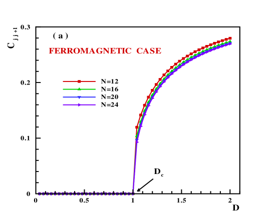
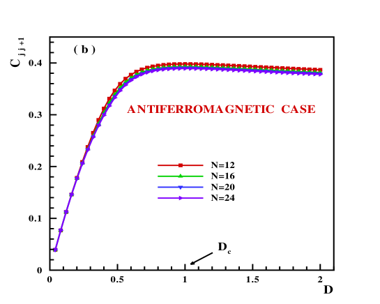
Figure 1: (Color online.) The concurrence is plotted as a function of DM vector $D$, (a) ferromagnetic and (b) antiferromagnetic cases for different lengths N=12, 16, 20, 24.

One-tangle and concurrence are related by Coffman-Kundu-Wootters (CKW) conjecture [32], which had been proved by Osborne and Verstraete [33], stating that

$$\tau_{1}\geq\tau_{2}\equiv\sum_{l\neq m}C_{lm}^{2}.$$ (6)

Which expresses the crucial fact that pairwise entanglement does not exhaust the global entanglement of the system, as entanglement can also be stored in 3-spin correlations, 4-spin correlations, and so on. Authors in Ref.([28, 29]), have proposed that, due to CKW conjecture, the minimum of the entanglement ratio $R\equiv\tau_{2}/\tau_{1}<1$, as a novel estimator of QPT, fully based on entanglement quantifiers.

By doing an experiment, one can find a clear picture of the entanglement phenomenon in the ground state magnetic phases of the model. Since a real experiment cannot be done at zero temperature, the best way is doing a virtual numerical experiment. A very famous and accurate method in the field of the numerical experiments is known as the Lanczos method. However, the strong role of a numerical experiment to examine quantum phase transitions is not negligible. To explore the nature of the entanglement in different magnetic phases, we used Lanczos method to diagonalize numerically chains with length up to $N=24$ and coupling constant $|J|=1$. The ground state eigenvector, $|Gs\rangle$, was obtained for chains with periodic boundary conditions. The numerical Lanczos results on the concurrence for the Ising chain with DM interaction, are shown in Fig. 1. As is clearly seen from Fig. 1(a), in the case of ferromagnetic chain and for $D<D_{c}=|J|=1$, the concurrence is equal to zero which shows that the ground state of the system is in the fully non-entangled polarized ferromagnetic phase. At the critical value $D_{c}=|J|=1$, the concurrence jumps to a non-zero value which confirms the metamagnetic phase transition. By more increasing the DM vector, $D>D_{c}$, the ground state is in the chiral phase and nearest neighbors are entangled. On the other hand, in the case of the antiferromagnetic Ising model, as can be clearly seen from Fig. 1(b), in the absence of the DM interaction, the ground state is non-entangled which is related to the saturated N$\acute{e}$el phase. As soon as the DM vector applies, nearest neighbors will be entangled and concurrence between them increases from zero. Thus in the case of antiferromagnetic Ising chains, the DM interaction induces the quantum correlations of the two spins and nearest neighbor spins will be entangled as soon as the DM interaction applies. In contrast, in the case of the ferromagnetic Ising chains the DM interaction only induces the quantum correlations after the critical value $D_{c}$ and nearest neighbor spins will not be entangled up to the critical value $D_{c}$.

An additional insight into the nature of different phases can be obtained by studying the entanglement ratio. Therefore, we have calculated the entanglement ratio by using Lanczos method in both ferromagnetic and antiferromagnetic cases. We have plotted our numerical results in Fig. 2. For ferromagnetic case, as it can be seen from Fig. 2(a), the entanglement ratio remains zero up to the critical DM interaction $D_{c}$ which is expected from the saturated ferromagnetic phase. As soon as the DM interaction increases from the critical $D_{c}$, the entanglement ratio starts to increase from zero. In the inset of Fig. 2(a), the first derivative entanglement ratio is plotted. As it is seen in the ferromagnetic phase, $D<D_{c}$, the derivative is equal to zero and an abrupt change took place exactly at $D_{c}=|J|=1$ which is an indication of the quantum phase transition. In the antiferromagnetic case, Fig. 2(b), as soon as the DM interaction applies the entanglement ratio creates and decreases by increasing the DM vector up to $D_{c}=1.0$ which a change took place and in the $D>D_{c}$ region the ratio becames monotonous. In the inset of Fig. 2(b), the first derivative entanglement ratio is plotted. It is clear that in the $D>D_{c}$ region derivative of ratio is equal to zero and an abrupt change took place exactly at $D_{c}=|J|=1.0$ which is an indication of the quantum phase transition.

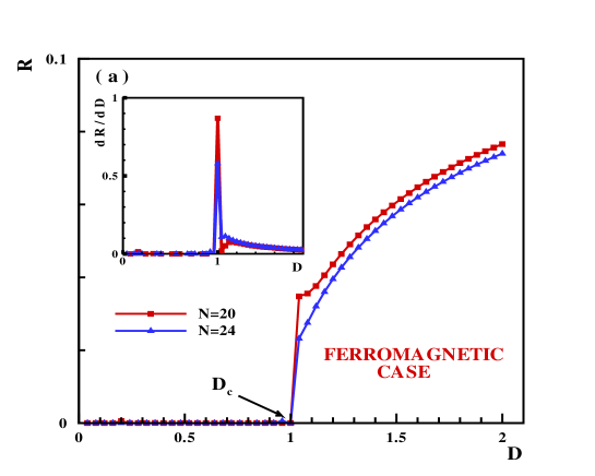
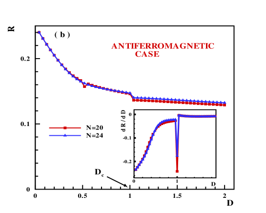
Figure 2: (Color online.) The entanglement ratio $\tau_{1}/\tau_{2}=R$ is plotted as a function of DM vector $D$, (a) ferromagnetic and (b) antiferromagnetic cases for different lengths N=20, 24. Inset: the first derivative of entanglement ratio.

2.2 Global Entanglement

Because of many different kinds of entanglement, quantifying of multipartite entanglement states (MES) is more difficult. Global-entanglement ($E_{gl}$) measure defined by Meyer and Wallach [34] which can measure the total nonlocal information per particle in a general multipartite system[35]

$$E_{gl}=\frac{1}{N}\left[2\sum_{i_{1}<i_{2}}\tau_{i_{1}i_{2}}+\cdot\cdot\cdot+N\sum_{i_{1}<\cdot\cdot\cdot<i_{N}}\tau_{i_{1}\cdot\cdot\cdot i_{N}}\right].$$ (7)

$E_{gl}$ is the average of tangles per particles ($\frac{<\tau>}{N}$ ), without giving detailed knowledge of tangle distribution among the individual particles. Therefore, $E_{gl}$ is an average quantity and cannot distinguish between entangled states which have equal $<\tau>$ yet different distributions of tangles, like $GHZ_{N}$ (Greenberger-Horne-Zeilinger) and $EPR^{\otimes N/2}$ state. $E_{gl}$ has ability to discriminate between $GHZ$ from $W$ states because of their different values of tangle. De Oliveira et al. [36] also introduced a slight extension of global entanglement as generalized global entanglement (GGE) which, in contrast to global entanglement, the proposed GGE measure can distinguish three paradigmatic entangled $GHZ_{N}$ (Greenberger-Horne-Zeilinger), $EPR^{\otimes N/2}$ and W states.

$$G(2,n) = \frac{4}{3}\frac{1}{N-1}\sum^{N-1}_{n=1}\left[1-\frac{1}{N-1}\sum^{N}_{j}Tr\rho^{2}_{j,j+n}\right]$$ (8)

$$= \frac{4}{3}\left[1-\frac{1}{4}\sum_{\alpha,\beta=0}^{3}\big{<}\sigma_{j}^{\alpha}\sigma_{j+1}^{\beta}\big{>}^{2}\right].$$

As such the generalized measure can detect a genuine multipartite entanglement and is maximal at the critical point[36]. Here, we have calculated multipartite entanglement Eq.(8) by using Lanczos numerical method with periodic boundary conditions in antiferromagnetic case. We have plotted our numerical results in Fig.3 for antiferromagnetic case. As it can be seen from Fig.3(a) the multipartite entanglement starts to increase by increasing DM up to the critical DM interaction $D_{c}$ which a change took place exactly at $D_{c}=|J|=1$ and then after that the multipartite entanglement reaches the saturation value. Our calculation shows that multipartite entanglement is maximal around the critical point $D_{c}$. In order to get better insight into the ability of multipartite entanglement as a quantum phase transition toolkit we have plotted the first derivative entanglement multipartite entanglement in the inset of Fig. 3(a). It shows divergent behavior at the critical point $D_{c}$. We have also plotted $lim_{n\rightarrow\infty}G(2,n)$ in Fig. 3(b). Our calculation shows $G(2,n)$ increases as $n\rightarrow\infty$ at the critical point. Here, we have finally calculated global entanglement $E_{gl}$ of model Eq.(1) and compar it with multipartite entanglement. It can be seen from Fig. 4 that both $G(2,n)$ and $E_{gl}$ are maximal at the critical point $D_{c}$ and their behavior is qualitatively the same.

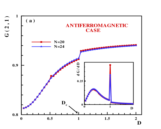
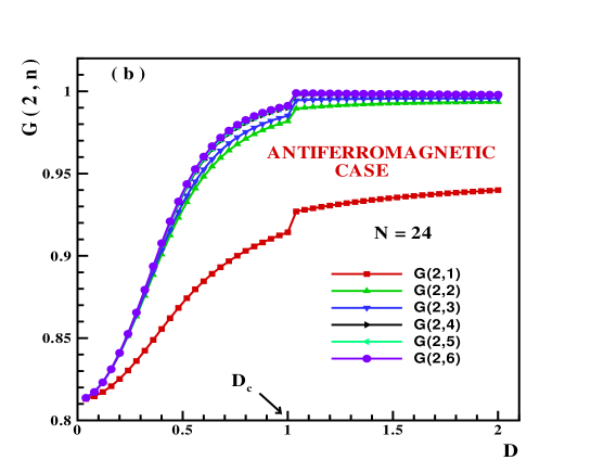
Figure 3: (Color online.) (a) Multipartite entanglement estimator $G(2,n)$ is plotted as a function of DM vector $D$ for antiferromagnetic Ising chain with length N=20, 24. Inset: the first derivative of multipartite entanglement$\frac{dG(2,n)}{dD}$. (b) $G(2,n)$ for the chain size N=24, is plotted in the limite of $n\rightarrow\infty$.

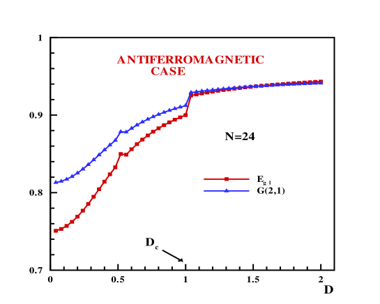
Figure 4: (Color online.) Multipartite entanglement $G(2,n)$ and global entanglement $E_{gl}$ are plotted as a function of DM vector $D$, for antiferromagnetic Ising chain with length N=24.

3 VARIATIONAL MATRIX PRODUCT STATE APPROACH

The matrix product state is defined as[37, 38]

$$|\psi\rangle=Tr(g_{1},g_{2},...,g_{N}),$$ (9)

where $g_{j}=a_{j}|\uparrow\rangle_{j}+b_{j}|\downarrow\rangle_{j}$, and $a_{j}$ and $b_{j}$ are probability amplitudes for two spin configurations at site $j$. In what follow, we intend to determine the ground state energy of ferromagnetic Ising spin system with DM interaction. In this respect, by using the above formalism, the variational energy is obtained by

$$E_{var}=\langle H\rangle=\frac{\langle\psi|H|\psi\rangle}{\langle\psi|\psi\rangle}=\sum_{j}\frac{\hat{H}_{j,j+1}}{[G_{j},G_{j+1}]},$$ (10)

where $\langle\psi|\psi\rangle=g_{1}\otimes g_{1}...g_{N}\otimes g_{N}=\Pi_{j}G_{j}$ and $G_{j}=g_{j}\otimes g_{j}=|a_{j}|^{2}+|b_{j}|^{2}$ here $\hat{H}_{jk}=J\hat{S}_{j}^{z}\hat{S}_{k}^{z}+\vec{D}.(\vec{S}_{j}\times\vec{S}_{k})$ and $\hat{S}_{j}^{\alpha}=g_{j}\otimes\vec{S}_{j}^{\alpha}g_{j}$. The minimum of the variational energy function corresponds to the ground state energy of the system. Using the normalization condition $\langle\psi|\psi\rangle=1$ , we can mapped variational parameter to $a_{j}=\cos(\theta_{j})e^{i\phi_{j}}$, $b_{j}=\sin(\theta_{j})e^{\acute{\phi_{j}}}$. Therefor one can obtain $\hat{S}_{j}^{z}=\frac{1}{2}\cos(2\theta_{j})$, $\hat{S}_{j}^{+}=(\hat{S}_{j}^{-})^{\dagger}=\frac{1}{2}\sin(2\theta_{j})e^{i\phi_{j}}$ where $\phi_{j}=\varphi_{j}-\acute{\varphi_{j}}$ and by choosing $\vec{D}=D\hat{z}$, it is found that:

$$E_{var} = \frac{1}{4}\sum_{j}\{J\cos(2\theta_{j})\cos(2\theta_{j+1})$$ (11)

$$+ D\sin(2\theta_{j})\sin(2\theta_{j})\sin(\phi_{j}-\phi_{j+1})\}.$$

By minimizing above equation, the ground state energy $(E_{GS})$ in the ferromagnetic case $J<0$ shall be obtained. It was shown that the ground state energy has the constant value, $E_{GS}=-\frac{N|J|}{4}$ for $D<|J|$ and decreasing linearly with DM interaction for $D>|J|$ as $E_{GS}=-\frac{ND}{4}$. Now, buy using the minimized variational parameters of $E_{var}$ we are able to calculate tangle Eq.(3) and concurrence Eq.(5). For $J>D$ one can obtain

$$g^{xx}_{j,j+1} = g^{zz}_{j,j+1}=g^{yx}_{j,j+1}=g^{xy}_{j,j+1}=0$$

$$g^{yy}_{j,j+1} = -1/4,$$ (12)

and $M^{z}=0$ so we have $\tau_{1}=1$ and $C_{j,j+1}=1/2$. For $J<D$ again using the above conditions, one can obtain

$$g^{xx}_{j,j+1} = g^{yy}_{j,j+1}=g^{yx}_{j,j+1}=g^{xy}_{j,j+1}=0$$

$$g^{zz}_{j,j+1} = 1/4,$$ (13)

and $M^{z}=1/2$ which give $\tau_{1}=0$ and $C_{j,j+1}=0$.

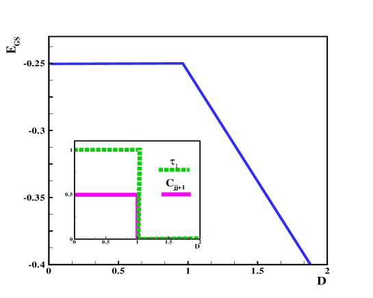
Figure 5: (Color online.) The ground state energy (normalized by N) of ferromagnetic Ising chain with DM interaction using variational matrix product state. Inset shows one-tangle and concurrence aas function of the DM interaction using variational matrix product state.

4 THREE-QUBIT ENTANGLEMENT

In this section we focus on the entanglement of formation of three-qubit in two inequivalent, symmetric and non-symmetric pairwise entanglement ways. By labeling the 3-qubits as $1,2,3$ sequentially. The symmetric reduced density matrix $\rho_{13}$ is defined as $\rho_{13}=tr_{2}(\rho)$, where $\rho$ is the density matrix of 3-qubits. The non-symmetric reduced matrix is $\rho_{12}=tr_{3}(\rho)$. Before present our results, we briefly review the definition of concurrence[15, 32]. Let $\rho_{ij}$ be density matrix of a pair of qubit $i$ and $j$. The concurrence corresponding to density matrix is defined as

$$C_{ij}=max\{\lambda_{1}-\lambda_{2}-\lambda_{3}-\lambda_{4},0\},$$ (14)

where the quantities $\lambda_{1}\geq\lambda_{2}\geq\lambda_{3}\geq\lambda_{4}$ are square roots of the eigenvalue of the operator

$$\varrho_{ij}=\rho_{ij}(\sigma_{y}\otimes\sigma_{y})\rho^{\ast}_{ij}(\sigma_{y}\otimes\sigma_{y}).$$ (15)

The concurrence $C_{ij}=0$ corresponds to an non-entangled state and $C_{ij}=1$ corresponds to a maximally entanglement sate. A straightforward calculation gives the eigenstates and the eigenvalues of 3-qubit of Eq.(1). The square roots of the operator $\varrho_{ij}$ for symmetric and nonsymmetric cases are presented in sequence. In the symmetric case $\varrho_{13}$

$$\lambda_{1}=0,\quad\lambda_{2}=\lambda_{3}=\left(\frac{\alpha^{2}}{\alpha^{2}+2}\right)^{2},\quad\lambda_{4}=4\left(\frac{2}{\alpha^{2}+2}\right)^{2}$$ (16)

and for the non-symmetric case $\varrho_{12}$

$$\lambda_{1}=\lambda_{2}=\left(\frac{1}{\alpha^{2}+2}\right)^{2},\quad\lambda_{3}=\left(\frac{(\alpha+1)^{2}}{\alpha^{2}+2}\right)^{2},\quad\lambda_{4}=\left(\frac{(\alpha-1)^{2}}{\alpha^{2}+2}\right)^{2}$$ (17)

where $\alpha=(J+\sqrt{8D^{2}+J^{2}})/2D$. In order to determine the existence of entanglement, we have considered ferromagnetic and antiferromagnetic cases. Fig.6 and Fig.7 show symmetric, $C_{13}$, and non-symmetric, $C_{12}$, concurrences. In the symmetric way, Fig. 6, it is clear that in the absence of DM interaction the antiferromagnetic case is entanglement, in contrast to ferromagnetic case which is fully unentangled. In antiferromagnetic case, the $C_{13}$ is zero up to $D_{c}=|J|$ and starts to increase by increasing DM and reaches a saturation value. Our calculation shows a competition between Ising exchange $J$ and the DM interaction which entanglement starts to decreasing by increasing Ising exchange. In the symmetric way, ferromagnetic Ising chain with added DM interaction does not show any entanglement and by increasing DM interaction nothing will not happen.

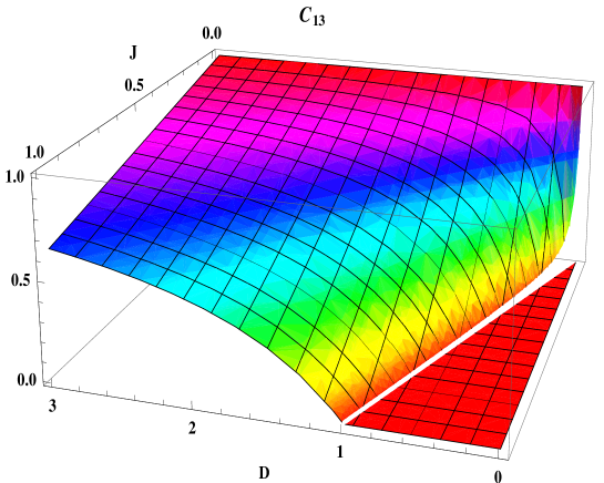
Figure 6: (Color online.) The ground state entanglement through symmetric way ,$C_{13}$, for antiferromagnetic case as function of DM and J exchange.

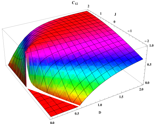
Figure 7: (Color online.) The ground state entanglement through non-symmetric way ,$C_{12}$, for both ferromagnetic an antiferromagnetic cases as function of DM and J exchange.

In the non-symmetric way, Fig. 7, ferromagnetic Ising chain with added DM interaction does not show any entanglement up to $D_{c}=|J|$. But for $D_{c}>|J|$ entanglement starts to increase by increasing DM interaction and shows a competitive behavior between DM and J exchange which entanglement shows decreasing by increasing $|J|$. In antiferromagnetic chain, through non-symmetric case, opposite to ferromagnetic case, is fully entangled. Entanglement starts to increasing from zero as soon as turn on DM and reaches its saturation value around $D_{c}=|J|$. It should be mentioned that in antiferromagnetic case, increasing $J$ exchange can enhance the amount of entanglement.

The concept of thermal entanglement was introduced and studied within one-dimensional isotropic Heisenberg model[39]. Here we study this kind of entanglement within three-qubit Ising chain with added DM interaction through symmetric and non-symmetric way. The state of the system at thermal equilibrium is $\rho(T)=\exp(-H/kT)/\Omega$, where $\Omega=Tr[\exp(-H/kT)]$ is the partition function and $k$ is the Boltezmann’s constant. As $\rho(T)$ represents thermal state, the entanglement in the state is called thermal entanglement[39]. The square roots of the operator $\varrho_{ij}(T)$ for symmetric and nonsymmetric cases are presented in sequence. For the non-symmetric case $\varrho_{13}(T)$

$$\lambda_{1}=\lambda_{2}=X_{12}^{2},\quad\lambda_{3}=\left(Y_{12}+Z_{12}\right)^{2},\quad\lambda_{4}=\left(Y_{12}-Z_{12}\right)^{2}$$ (18)

where

$$X_{12} = \frac{1}{\Omega}\left[\frac{1}{2}+\frac{e^{-\beta\varepsilon_{3}}}{a^{2}+2}+e^{-\beta\varepsilon_{5}}+\frac{e^{-\beta\varepsilon_{7}}}{b^{2}+2}\right],$$

$$Y_{12} = \frac{1}{\Omega}\left[\frac{1}{2}+\frac{(a^{2}+1)e^{-\beta\varepsilon_{3}}}{a^{2}+2}+\frac{(b^{2}+1)e^{-\beta\varepsilon_{7}}}{b^{2}+2}\right],$$

$$Z_{12} = \frac{1}{\Omega}\left[\frac{2ae^{-\beta\varepsilon_{3}}}{a^{2}+2}+\frac{2be^{-\beta\varepsilon_{7}}}{b^{2}+2}\right],$$ (19)

and for the non-symmetric case $\varrho_{12}(T)$

$$\lambda_{1}=\lambda_{2}=X_{13}^{2},\quad\lambda_{3}=\left(Y_{13}+Z_{13}\right)^{2},\quad\lambda_{4}=\left(Y_{13}-Z_{13}\right)^{2}$$ (20)

where

$$X_{13} = \frac{1}{\Omega}\left[\frac{a^{2}e^{-\beta\varepsilon_{3}}}{a^{2}+2}+e^{-\beta\varepsilon_{5}}+\frac{b^{2}e^{-\beta\varepsilon_{7}}}{b^{2}+2}\right],$$

$$Y_{13} = \frac{1}{\Omega}\left[1+\frac{(2e^{-\beta\varepsilon_{3}}}{a^{2}+2}+\frac{2e^{-\beta\varepsilon_{7}}}{b^{2}+2}\right],$$

$$Z_{13} = \frac{1}{\Omega}\left[1-\frac{(2e^{-\beta\varepsilon_{3}}}{a^{2}+2}-\frac{2e^{-\beta\varepsilon_{7}}}{b^{2}+2}\right],$$ (21)

and $\Omega=4e^{-\beta J}[\cosh\beta J+\cosh\beta\sqrt{8D^{2}+J^{2}}]$, $a=J-\sqrt{8D^{2}+J^{2}}/2D$, $b=J+\sqrt{8D^{2}+J^{2}}/2D$. In Fig.8 and Fig.9 we give two plots of the thermal concurrence of antiferromagnetic and ferromagnetic Ising chains as functions of temperature and DM interaction respectively. In antiferromagnetic case, Fig.8, model dose not shows any entanglement through symmetric way and model lives in fully unentangled phase. In contrast to symmetric way, non-symmetric way shows entanglement. As it can be seen from Fig.8, there is a region which surprisingly temperature can enhance entanglement and this region will become wide spread for higher DM. For higher temperature DM can not overcome temperature and entanglement gradually goes to zero by increasing temperature.

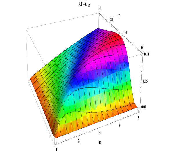
Figure 8: (Color online.) The thermal entanglement through non-symmetric way ,$C_{12}$, for antiferromagnetic case as function of DM and temperature.

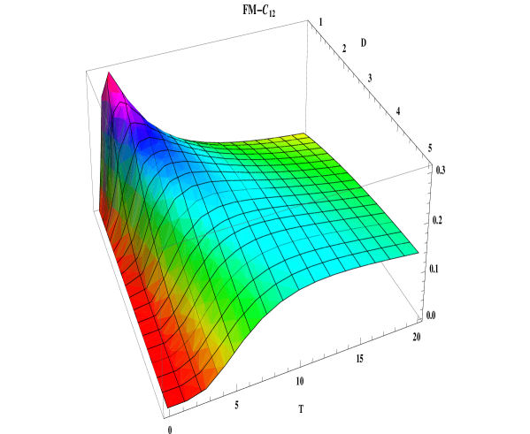
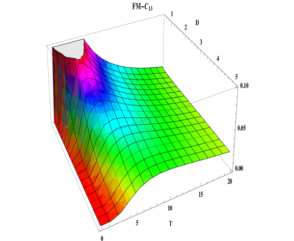
Figure 9: The thermal entanglement through non-symmetric way(top) ,$C_{12}$, and symmetric way(bottom) ,$C_{13}$,for ferromagnetic case as function of DM and temperature.

In ferromagnetic case, Fig.9, both symmetric and non-symmetric way have qualitatively the same behavior. Here, same as antiferromagnetic case, temperature can enhance entanglement. Thermal and quantum fluctuations have a tight competition to drive system in favorable regime, but in low temperature, both temperature and DM interaction has effective influence on the degree of entanglement of the system and both of them could be used to increase the entanglement of the spin system.
Either Fig.6 and Fig.7 are plotted for $D>D_{c}=1$, because we could not find any prominent behavior for $D<D_{c}=1$. Actually both symmetric and non-symmetric entanglement are zero in the $D<D_{c}=1$ region.

5 CONCLUSION

To summarize, we have investigated the effect of a Dzyaloshinskii-Moriya (DM) interaction on the ground state phase diagram of the one-dimensional (1D) Ising spin-1/2 model using the variational matrix product state and numerical Lanczos methods from entanglement point of view. Our results show that there is a critical point in either ferromagnetic and antiferromagnetic cases. In the ferromagnetic Ising chain this critical point was predicted by variational matrix approach exactly at $D_{c}=|J|$, which by using numerical study we have confirmed it. We have also used the minimum of the entanglement ratio $R\equiv\tau_{2}/\tau_{1}<1$,to check the presence of this quantum critical point. For both ferromagnetic and antiferromagnetic cases our numerical study gave the minimum of $R\equiv\tau_{2}/\tau_{1}$ at $D_{c}=|J|$,. We also used generalized multipartite entanglement tools to check how entanglement is share in our model and check their ability to detect critical point. For antiferromagnetic case we have calculated global $E_{gl}$ and generalized multipartite entanglement $G(2,n)$ and either of them show that a quantum phase transition took place at $D_{c}=|J|$ .

We have calculated ground state entanglement of symmetric, $C_{13}$, and non-symmetric, $C_{12}$, concurrences for ferromagnetic and antiferromagnetic cases. In the symmetric way, in the absence of DM interaction both antiferromagnetic and ferromagnetic cases are fully unentangled. By increasing DM, in antiferromagnetic case, the $C_{13}$ is zero up to critical points $D_{c}=|J|$. After the critical point entanglement starts to increase until its saturation. For ferromagnetic case, in symmetric way $C_{13}$ is always zero and does not show any entanglement.

In the non-symmetric way, in the absence of DM interaction, $C_{12}$ is equal zero for either antiferromagnetic and ferromagnetic cases. By turning DM nothing, in the ferromagnetic case, will not happen up to critical point $D_{c}$ and then after that $C_{12}$ starts to increase by increasing DM interaction. In contrast to ferromagnetic case, in the antiferromagnetic case $C_{12}$ starts to increasing immediately after turning DM and reaches its saturation value around $D_{c}=|J|$.

We have also studied thermal entanglement of symmetric, $C_{13}(T)$, and non-symmetric, $C_{12}(T)$ for both ferromagnetic and antiferromagnetic cases. Our calculations show that for either symmetric and non-symmetric cases thermal(unentanglement favorable) and quantum(entanglement favorable) fluctuations have competition to drive system to their favorable regime and surprisingly thermal decoherence can enhance entanglement in some part of low temperature region.

References

References

- [1] Nielsen M A and Chuang I L 2000 Quantum Computation and Quantum information, Cambridge University Press
- [2] Wang X 2001 Phys. Rev. A 64, 012313
- [3] Arnesen M C, Bose S and Vedral V 2001 Phys. Rev. Lett. 87 , 017901
- [4] Osborne T J, Nielsen M A 2002 Phys.Rev. A 66, 032110
- [5] Osterloh A, Amico L, Falci G and Fazio R 2002 Nature 416, 608
- [6] Vidal G, Latorre J I, Rico E and Kitaev A 2003 Phys. Rev. Lett. 90, 227902
- [7] Wu L A, Sarandy M S and Lidar D A 2004 Phys.Rev.Lett. 93, 250404
- [8] Dur W, Hartmann L, Hein M, Lewenstein M and Briegel H J 2005 Phys.Rev.Lett. 94, 097203
- [9] Guhne O, Toth G, Briegel H J 2005 New J. Phys. 7, 229
- [10] Lou P and Lee J Y 2006 Phys. Rev. B 74, 134402
- [11] Amico L, Fazio R, Osterloh A and Vedal V 2008 Rev. Mod. Pys. 80, 517
- [12] Horodecki R, Horodecki P, Horodecki M and Horodecki K 2009 Rev. Mod. Phys. 81, 865
- [13] Sachdev S 2000 Quantum Phase Transitions (Cambridge University Press, Cambridge, UK ).
- [14] Osterloh A et al. 2002 Nature (London) 416, 608
- [15] Wooters W K 1998 Phys. Rev. Lett. 80, 2245
- [16] Vidal G and Werner R F 2002 Phys. Rev. A 65, 032314
- [17] Dzyaloshinsky I 1958 J. Phys. Chem. Solids 4, 241
- [18] Moriya T 1960 Phys. Rev. Lett. 4, 228
- [19] Sudan J, Luscher A and Lauchli A M 2009 Phys. Rev. B 80, 140402(R)
- [20] Seki S, Yamasaki Y, Soda M, Matsuura M, Hirota K and Tokura Y 2008 Phys. Rev. Lett. 100, 127201
- [21] Huvonen D, Nagel U, Room T, Choi Y J, Zhang C L, Park S and Cheong S W 2009 Phys. Rev. B 80, 100402(R)
- [22] Oshikawa M and Affleck I 1999 Phys. Rev. Lett. 82, 5136; Affleck I and Oshikawa M 1999 Phys. Rev. B 60, 1038
- [23] Derzhko O, Verkholyak T, Krokhmalskii T and Buttner H 2006 Phys. Rev. B 73, 214407
- [24] Kargarian M, Jafari R and Langari A 2009 Phys. Rev. A 79, 042319
- [25] Garate I and Affleck I 2010 Phys. Rev. B 81, 144419
- [26] Soltani M R, Mahdavifar S, Akbari A, Masoudi A A 2010 J. Sup and Nov. Mag, 23, 1369
- [27] Jafari R, Kargarian M, Langari A and Siahatgar M 2008 Phys. Rev. B 81, 054413
- [28] Roscilde T, Verrucchi P, Fubini A, Haas S and Tognetti V 2004 Phys. Rev. Lett. 93, 167203
- [29] Roscilde T, Verrucchi P, Fubini A, Haas S and Tognetti V 2005 Phys. Rev. Lett. 94, 147208
- [30] Bennett C H, DiVincenzo D P, Smolin J A and Wootters W K 1996 Phys, Lett. A 54, 3824
- [31] Amico L, Osterloh A, Plastina F, Fazio R and Palma G M 2004 Phys, Lett. A 69, 022304
- [32] Coffman V, Kundu J and Wootters W K 2000 Phys. Rev. A 61 052306
- [33] Osborne T J and Verstraete F 2006 Phys, Rev, Lett 96, 220503
- [34] Meyer D A and Wallach N R 2002 J. Math. Phys. 43, 4273
- [35] Montakhab A and Asadian A 2010 Phys. Rev. A 82, 062313
- [36] de Oliveira T R, Rigolin G, de Oliveira M C 2006 Phys. Rev. A 73, 010305(R); Rigolin G, de Oliveira T R, de Oliveira M C 2006 Phys. Rev. A 74, 022314 ; de Oliveira T R, Rigolin G, de Oliveira M C and Miranda E 2006 Phys. Rev. Lett. 97, 170401
- [37] Klumper A, Schadschneider A and Zittartz 1991 J. Phys. A 24, L955 ; Klumper A, Schadschneider A and Zittartz 1992 Z. Phys. B 87, 281 ; Klumper A, Schadschneider A and Zittartz 1993 Europhys. Lett. 24, 293
- [38] Fannes M, Nachtergaele B and Werner R F 1989 Europhys. Lett. 10, 633
- [39] Arnesen M C, Bose S and Verdal V 2001 Phys. Rev. Lett. 87, 017901; Nielsen M A 1998 PhD Dissertation, The University of New Mexico