Single pulse analysis of PSR B1133+16 at 8.35 GHz and carousel circulation time

Abstract

A successful attempt was made to analyse about 6000 single pulses of PSR B1133+16 obtained with the 100-meter Effelsberg radio–telescope. The high resolution (60 micro-seconds) data were taken at a frequency of 8.35 GHz with a bandwidth of 1.1 GHz. In order to examine the pulse-to-pulse intensity modulations, we performed both the longitude– and the harmonic–resolved fluctuation spectral analysis. We identified the low frequency feature associated with an amplitude modulation at $f_{4}\simeq 0.033P_{1}^{-1}$, which can be interpreted as the circulation time $P_{4}\simeq 30P_{1}$ of the underlying subbeam carousel model. Despite an erratic nature of this pulsar, we also found an evidence of periodic pseudo-nulls with $P_{4}=28.44P_{1}$. This is exactly the value at which Herfindal & Rankin found periodic pseudo-nulls in their 327 MHz data. We thus believe that this is the actual carousel circulation time in PSR B1133+16, particularly during orderly circulation.

1 Introduction

Generally pulsars are weak radio sources, and even with the sensitivity of current radio telescopes single pulses are observable only from the strongest objects. Due to the steep spectrum of pulsar radio–emission, single pulse observations were readily made at low frequencies, where the sensitivity requirements for antenna and receiver systems were not an issue. PSR B1133+16 is one of the brightest pulsars in the northern hemisphere (32 mJy at 1.4 GHz, spectral index of $-1.5$ Maron et al., 2000). Individual pulses of PSR B1133+16 were recorded during numerous observing campaigns, and analyses of single pulse behaviour were performed at the observing frequencies from 110 MHz to 1.4 GHz (Backer, 1973; Taylor, Manchester & Huguenin, 1975; Nowakowski, 1996; Weltevrede et al., 2006, 2007; Herfindal & Rankin, 2007). With the recent development of high sensitivity receivers, and given the fact that PSR B1133+16 is a relatively strong source, measurements of its single pulses with high time resolution were possible at frequencies as high as 8.35 GHz.

The most common feature revealed by single-pulse sequences is related to the phenomenon of drifting subpulses (Drake & Craft, 1968; Sutton et al., 1970; Weltevrede et al., 2007). The parameters of the drift were first described by Backer (1973), later modified by Gil & Sendyk (2003) and Gupta et al. (2004). The first of the four main periodicities involved is the basic pulsar (spin) period $P_{1}$, i.e. the interval between our successive sampling of the pulsar beam. The overall pulsar beam is organized into a number of subbeams, only some of which cross our sightline during any given pulse, and thus directly correspond to the number and the locations of subpulses we observe. The second periodicity, $P_{2}$, is the angular distance between adjacent subpulses, or the corresponding subbeams, as viewed along rotational longitude. The magnetic azimuthal separation, say $\eta$, between adjacent subbeams implied by $P_{2}$ can be estimated (e.g., see Eq. 3 of Deshpande & Rankin, 2001). For $N$ subbeams, when evenly placed within the emission cone, $\eta$ would be $=360^{\circ}/N$. The next period $P_{3}$ (usually measured in units of $P_{1}$, and as per its initial definition) is the distance between adjacent drift bands, or in other words, the interval after which the subsequent subbeam reaches the same phase as the preceding one. In case of fast drifts, however, one has to take into account possible aliasing effect, which can cause a large degree of ambiguity. Fluctuation spectral analysis can help to resolve the aliasing issue, and is therefore commonly used. In such Fourier analysis, the periodic phase modulation associated with the subpulse drift manifests as a spectral feature at the corresponding fluctuation frequency, $f_{3}\equiv 1/P_{3}$. This feature is usually seen at relatively high fluctuation frequencies, and hence, often called the high frequency feature (HFF). Finally, we can introduce the total circulation time of the pattern, or the interval after which a given subbeam reaches the same phase, $P_{4}$ ($\hat{P}_{3}$ in Ruderman & Sutherland, 1975, RS75 henceforth, who introduced this feature theoretically). The circulation time becomes measurable if the subbeams vary in intensity, as they most often do, and such periodic amplitude modulation would be apparent as an accompanying spectral feature at frequency $f_{4}\equiv 1/P_{4}$. This spectral feature, when present, is invariably located in the lower band of the fluctuation spectrum, and is referred to as the low frequency feature (LFF). According to the carousel model, first introduced by RS75 and developed by Deshpande & Rankin (1999, 2001) and Gil & Sendyk (2000, 2003), the two periodicities $P_{3}$ and $P_{4}$ are connected to each other via a direct relationship $P_{4}=NP_{3}$.

PSR B1133+16 apparently shows the phenomenon of drifting subpulses, although it was shown that the organized character of the subplulses appears only for some finite timespans, outside of which the behaviour of the individual pulses is highly chaotic. Recently Weltevrede et al. (2007) detected the high-frequency (phase-modulation) spectral feature corresponding to period of $P_{3}=(3\pm 2)P_{1}$. Moreover, they also detected a low-frequency (amplitude-modulation) feature corresponding to period $P_{4}=(30\pm 8)P_{1}$. The very large uncertainty in the former estimate follows from a fact that the authors were not able to resolve the issue of aliasing in their analysis. Herfindal & Rankin (2007, HR07 henceforth) attempted to resolve the aliasing problem and demonstrated that the actual $P_{3}=(1.237\pm 0.011)P_{1}$. Their spectral and profile-folding analyses confirmed the existence of the low-frequency feature (LFF) in the spectrum, corresponding to a period of $P_{4}=28.44P_{1}$. The unprecedented accuracy of the latter estimate is a result of sophisticated analysis, including the cartography technique developed by Deshpande & Rankin (1999, 2001), as well as detection of periodic pseudo-nulls of very short duration. It is worth noting that the value of N=28.44/1.237 is exactly 23 in their analysis, as it supposed to be for a parameter describing the number of subbeams contributing to the observed drifting subpulse phenomenon. Thus, the value of $P_{4}=28.44P_{1}$ represents the carousel circulation time in PSR B1133+16 (HR07).

In this paper we attempt to find the pulse modulation features using spectral analysis of our high frequency (8.35 GHz), high time resolution (60 $\mu$s) single pulse data of PSR B1133+16.

2 Observations and Data Analysis

Our observations of single pulses of PSR B1133+16 were made with the 100-meter radio telescope of Max-Planck Institute for Radioastronomy in 2004. We used a cooled secondary-focus receiver equipped with HEMT amplifiers, with an observing frequency of 8.35 GHz and 1.1 GHz bandwidth. The pulsar signal was recorded by Effelsberg Pulsar Observations System (EPOS, Jessner, 1996), with a time resolution of 60 micro-seconds. To achieve the best pulse coverage, we used a gating system, in which 1024 bins were used to cover only about 5% of the pulse period around the main pulse. Data were gathered during two separate 60-minute sessions (c.a. 3000 pulses each).

Figure 1 shows a sample of the data we gathered; a set of 256 consecutive individual pulses, with its average pulse profile at the top. One can see that only some of the individual pulses were clearly detected. For a majority of the pulses, the radio emission was very weak or even missing. Naturally, the typical phenomena related to subpulse drifting, like the appearance of drift bands or high-frequency features in the modulation spectra, may not be readily apparent. However, contrary to our low expectations, we managed to detect all periodicities appearing in the pulse intensity modulations visible in better quality low-frequency data. The level of confidence of these detections varied between different segments of the data set. For example, a low-frequency amplitude-modulation feature was very prominent in the analysis of one set of pulses, while in some sets the feature can be recognized in the spectrum, but not at a level sufficient to claim a clear detection. However, the particular set (segment B; pulses 512-768) shown in Figure 1 is one of our best-quality intervals, where the periodic intensity modulation, with $P_{4}$ close to 28 $P_{1}$, is clearly visible.

Figure 1: A sequence of pulses from 512th to 768th pulse from observation B, showing clearly a periodic intensity modulation (conf. Tables 1 and 2). The thick line at the top represents the integrated profile for this sequence.

2.1 Longitude–Resolved Fluctuation Spectra

In order to analyse the gathered data, we used the method of Longitude-Resolved Fluctuation Spectra (LRFS hereafter, Backer, 1970), which detects the regularities in the intensity variations of individual pulses. To implement the method, we divided the pulse series into blocks of 256 pulses, and performed the one-dimensional fast Fourier transform (FFT) for each longitude bin, and computed the power spectrum. The spectra were then normalized for each individual longitude bin, resulting in 1024 independent power spectra. These were then summed to form an integrated power spectrum separately for each of the 256-pulse stacks.

A feature with periodicity around 2.85 $P_{1}$ was identified in the fluctuation spectra at all longitudes, as well as in the integrated spectrum. This feature was present in all our pulse sequences, and it’s origin was traced down to the AC power line. We confirmed that this feature was not associated with the pulsar signal by obtaining LRFS for the off-pulse region. The feature was extremely strong, potentially masking any real features present in the contaminated part of the spectrum. Therefore, we decided to remove it from the fluctuation spectra. To achieve this, we reconstructed a continuous time series from the available gated data and calculated its FFT. In this fluctuation spectrum, we replaced the values at the locations corresponding to the fundamental frequency of the contaminant, and its harmonics (separated by the pulsar frequency as a consequence of the gating), with zeros. An inverse Fourier transform of thus edited spectrum yielded a modified time series, free of this interference, which after the re-application of gating allowed us to repeat the LRFS analysis.

2.2 Harmonic resolved fluctuation spectra

The LRFS gives us a wealth of information about the fluctuations present in the sequence, but also has a serious drawback of aliasing due to poor sampling of fluctuations at a given longitude only once every pulse period. In order to deal with the issue of aliasing, we need to overcome the basic limitation of this sampling. Noting that the fluctuations are sampled more than once in the finite duration of the pulse, one can combine the fluctuation spectra of the different longitude bins with appropriate phases corresponding to the longitude separation to obtain the Harmonic-Resolved Fluctuation Spectra (HRFS hereafter). This approach was used and developed by Deshpande & Rankin (1999, 2001). In practice, this is achieved by Fourier transforming the entire continuous sequence, which can be reconstructed (from the gated version) by using the available on-pulse samples, and filling the rest of the longitude regions with zeros. In this process, the pulse sequence is effectively multiplied by a periodic window function which leads to convolution of the spectrum associated with the un-gated pulse sequence with the Fourier transform of the periodic window (gating) function used.

3 Results

We analysed several 256-pulse (c.a. 300 second) data blocks from both of our 60-minute observations (we call them $A$ and $B$ for the purposes of referencing here). For some of these blocks, we have identified a prominent low frequency feature (LFF) in the integrated spectra obtained with LFRS, as well as HRFS, analysis.

Figure 2 shows the result of our LRFS analysis for an interference-cleaned 256-pulse stack, and Table 1 lists the values of the measured frequency $f_{4}$ of the LFF and the corresponding periodicity $P_{4}=1/f_{4}$ for those data blocks in which these features were detected using the LRFS analysis. For the remaining data blocks the LFF was either not present at all (no identifiable peaks close to this frequency in the power spectrum), or its signal-to-noise ratio was too small to claim its presence beyond doubt (usually due to other features that appeared in the power spectrum). The $f_{4}$ values corresponding to the LFF vary between the blocks, but stay consistent within the estimated uncertainties.

For the observation $A$, it was possible to identify the LFF in the average spectrum, obtained as a sum of the spectra from all the data blocks. The value of the LFF frequency from the average spectrum (see Table 1) was close to the $28.44P_{1}$ obtained by HR07 as the putative circulation time of their carousel solution. The same was not possible for observation $B$, as the LFF frequency varies significantly from block to block, resulting in a smearing of the feature in the averaged spectrum. However, it is worth noting that in the best block B (512-768, see Fig. 1) with the lowest estimated errors, the $P_{4}=(28.4\pm 1.2)P_{1}$ was also very close to the HR07 value. Table 1 also contains the weighted average of the LFF period, obtained from all individual block measurements.

The result of our HRFS analysis of the same 256-pulse sequence (as used for the LFRS in Fig. 2) is shown in Fig. 3. The HRFS for these pulse sequences also show the LFF, usually with another feature (at the frequency equal to 1.0 minus the LFF frequency; conf. Figure 3), which would be expected to be present as the LFF’s symmetric counterpart (as in a pair of sidebands about each of the pulsar harmonics) in case of amplitude modulation. The results of the measurement of the LFF parameters (see Table 2) agree with those from the LRFS analysis. Similar to the case with LRFS, we were able to find the LFF in the average HRFS only for the observation $A$, and the estimated weighted-average frequency (and the corresponding period) associated with the LFF are also presented in Table 2.

Table 1: Parameters of the observed low-frequency feature (LFF) obtained from the LRFS analysis. Table includes also the value obtained from the average spectrum of the whole observation A, as well as the weighted average of the LFF frequency, and the value of $P_{4}$ based on it (in parentheses).

Observation	Pulse	LFF
	sequence	Period $[P_{1}]$	Freq. $[P_{1}^{-1}]$
A	1-256	28.4$\pm$3.3	$0.035\pm 0.004$
A	512-768	28.4$\pm$3.5	$0.035\pm 0.004$
A	2109-2365	32.0$\pm$2.2	$0.031\pm 0.002$
B	1-256	36.5$\pm$4.5	$0.027\pm 0.003$
B	512-768	28.4$\pm$1.2	$0.035\pm 0.002$
B	2304-2560	34.6$\pm$9.5	$0.029\pm 0.007$
Freq. weighted average		(30.9$\pm$1.1)	$0.0323\pm 0.0012$
Average spectrum of A⋆		28.3$\pm$7.2	$0.035\pm 0.009$
⋆ - see text in Section 3 for details.

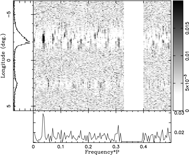
Figure 2: Longitude-resolved fluctuation spectrum for PSR B1133+16 computed for 8.35 GHz observations (using the sequence from 1st to 256th pulse from observation A). The main panel presents, in grey-scale, the full fluctuation spectrum for all longitude bins corresponding to the integrated pulse profile, which is shown in the left hand panel. The bottom panel presents the integrated fluctuation spectrum; note the prominent feature close to 0.03$P_{1}^{-1}$. This feature is clearly visible also in the LRFS corresponding to the leading bright pulse component. The white band visible in the LRFS greyplot is a result of removal of a whole range of frequencies that were distorted by AC power line interference.

Table 2: Parameters of the observed low-frequency feature (LFF) obtained from the HRFS analysis. Table includes also the value obtained from the average spectrum of the whole observation A, as well as the weighted average of the LFF frequency, and the value of $P_{4}$ based on it (in parentheses).

Observation	Pulse	LFF
	sequence	Period $[P_{1}]$	Freq. $[P_{1}^{-1}]$
A	1-256	28.4$\pm$3.1	0.035$\pm$0.004
A	512-768	32.0$\pm$4.6	0.031$\pm$0.004
A	2109-2365	32.0$\pm$2.3	0.031$\pm$0.002
B	1-256	36.5$\pm$6.3	0.027$\pm$0.005
B	512-768	28.4$\pm$3.0	0.035$\pm$0.004
B	2304-2560	32.0$\pm$8.8	0.031$\pm$0.010
Freq. weighted average		(31.5$\pm$1.4)	0.0317$\pm$0.0014
Average spectrum of A⋆		25.6$\pm$3.3	0.039$\pm$0.005
⋆ - see text in Section 3 for details.

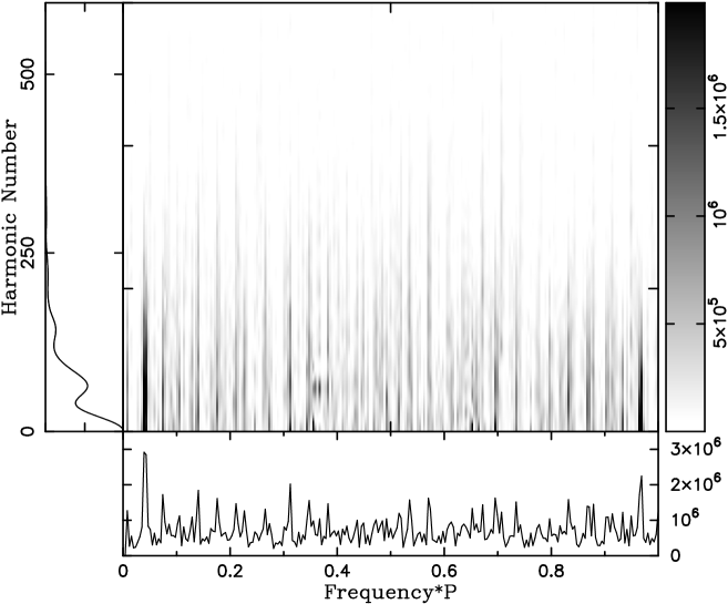
Figure 3: Harmonic-resolved fluctuation spectrum for PSR B1133+16 computed for the 8.35-GHz observations. The grey-scale plot in the central panel shows the full spectrum, and the bottom panel - the integrated spectrum. In both of them, two features clearly stand out - one close to $0.03P_{1}^{-1}$, which is the low frequency feature (LFF), and its symmetric counterpart at $\sim 0.97P_{1}^{-1}$. The contributions, shown in the main panel, corresponding to any given frequency appear stretched along the harmonic-number axis. This is an anticipated consequence of periodic windowing, including the natural pulse-shape mask and any deliberate windowing, such as gating. Left panel shows the relative strengths of pulsar frequency harmonics (equivalent to the Fourier transform of the average pulse profile). The presented spectrum was obtained for the same sequence of 256 pulses, as used for the LFRS in Fig. 2 (i.e. the first 256 pulses from observation A). One has to remember that, for the purpose of HRFS analysis, we had to reconstruct a continuous time series from the available gated observations.

4 Discussion and Conclusion

The average fluctuation frequency of the LFF , that we identified (in selected segments of our data), corresponds to a period of $(31.5\pm 1.4)P_{1}$ (see Table 2). We have chosen the value calculated by the means of HRFS analysis as the best representative for a number of reasons (although one has to note that values from LRFS and HRFS agree well within the error estimates). First of them is that HRFS adds the contribution associated with the modulations potentially coherently, using the implicit connection between modulation seen at different longitudes, as against the incoherent addition of modulations contribution across longitudes in LRFS. The former therefore is expected to provide a higher signal-to-noise ratio for coherent modulations, than the latter case. Also, while in case of HRFS the spectral power is divided between the feature and its alias, for amplitude modulated features the same goes for LRFS analysis, we just do not look at the negative part of the spectrum. And finally, having two separated, but related features (alias frequency is 1 minus LFF frequency) allows for more precise measurement of the LFF position in the spectrum.

The value we obtained is consistent with other single-pulse studies of PSR B1133+16 (see Table 3). More importantly, a few segments of the best quality data show $P_{4}$ close to $28.44P_{1}$, the value given by HR07. They estimated this refined value of $P_{4}$ using profile folding over the circulation period, which is desirably sensitive to periodic pseudo-nulls.

Our data do not show a direct evidence of the HFF corresponding to subpulse drift because of the erratic nature of the individual pulses (see Fig. 1); this is quite normal behaviour for this pulsar, which is - at our observing frequency of 8.35 GHz - amplified by the fact, that most of the incoming pulses remain below our detection threshold. Since $P_{3}$ (aliased or not) measures the distance between subpulse drift bands, it is clear that in our data, where most of the pulses are missing, this periodicity cannot be easily detected. In addition one has to remember, that even at lower observing frequencies, the drifting subpulse phenomenon is not always present. However, one should not ignore a putative drift feature at frequency about 0.81 $P_{1}^{-1}$, that we found in selected segments of our data (hidden in a forest of features in the average HRFS spectrum), which corresponds to the periodicity of about $P_{3}=1.237P_{1}$. We note its similarity to Fig. A1 in HR07, where this drift feature at frequency about 0.81 $P_{1}^{-1}$ is clearly present. It is also worth noting that $P_{4}/P_{3}=28.44/(1.23\pm 0.01)$ is exactly 23, which represents the number of circulating beamlets in the carousel model of HR07.

There is no fundamental reason why the LFF corresponding to amplitude modulation also should be weak or even missing in our data. Even when the sub-pulse phase behavior is less ordered, and the primary phase fluctuation feature (HFF) may not be apparent in the spectrum, the low-frequency feature indicative of circulation period may stand out clearly representing the overall intensity variation across magnetic azimuth. The first of such examples of LFF was discussed by Asgekar & Deshpande (2001, 2005) based on their low-frequency (35 MHz) data of B0943+10 and B0834+06. Also, a very good example is the so-called Q-mode in PSR B0943+10 analysed by Rankin & Suleymanova (2006) in their 327-MHz Arecibo data. Unlike in the regular B-mode of this pulsar with driftbands clearly visible and the HFF appearing in the fluctuation spectrum, single pulses in the Q-mode are completely chaotic, and no driftbands appear in pulse sequences (see Fig. 4 in Rankin & Suleymanova, 2006). Still, in this mode, the LFF corresponding to carousel circulation time is clearly visible in the fluctuation spectrum (see Fig. 6 in Rankin & Suleymanova, 2006). Yet another example of pulsars with erratic subpulses, but nevertheless showing the LFF that can be interpreted as the carousel circulation time, is PSR B0656+14 (see footnote 1).

It is interesting and important that we are able to identify the LFF in our erratic data using both, LRFS as well as HRFS analysis. The LRFS does not, however, resolve the issue of whether the apparent spectral feature is indeed the true one or is an alias of another feature outside of the unaliased frequency range. The HRFS, on the other hand, can help resolve such ambiguity to a large extent, and therefore we believe the estimate of the frequency from the HRFS to be more reliable. Moreover, the HRFS analysis provides additional clues about the nature of modulation.

Previous studies reported an LFF at $f_{4}\simeq 0.033P_{1}^{-1}$ (see references in Table 3). In our HRFS spectra (see Fig. 3), we also clearly see this feature as the most prominent one. There is also another significant feature at frequency $0.967P_{1}^{-1}$, which is certainly the counterpart of the LFF ($0.033P_{1}^{-1}$) (see also Fig. A1 in Herfindal & Rankin, 2007). We thus believe that the true frequency $f_{4}$ is indeed about 0.033 $P_{1}^{-1}$, and the roughly similar intensities (within uncertainties) of the two spectral features are to be interpreted as suggesting significant amplitude modulation rather than phase modulation (which would be the characteristic of drifting subpulses). In any case, the prominence of the LFF in comparison with its harmonics indicates a rather systematic (non-random) and possibly smooth variation of intensity across the pattern of subbeams.

Table 3: Results of observed Low Frequency Feature in PSR B1133+16 found in the literature and from our analysis

References	Observation	Period from LFF
	frequency	(in units of $P_{1}$)
Slee & Mulhall (1970)	80 MHz	37$\pm 15$
Karuppusamy, Stappers	110 - 180 MHz	30$\pm$5
& Serylak (2011)		$34^{+5}_{-3}$
Taylor & Hugenin (1971)	147 MHz	27.8
Weltevrede et al. (2006)	326 MHz	$30\pm 8$
Herfindal, Rankin (2007)	327 MHz	32$\pm$2
Nowakowski (1996)	430 MHz	32
Backer (1973)	606 MHz	37
Weltevrede et al. (2007)	1.4 GHz	33$\pm$5
Our Analysis (HRFS)	8.35 GHz	32$\pm$2

Gil, Melikidze & Zhang (2006, GMZ06 henceforth) claimed that, in the case of PSR B1133+16, the LFF reported in the literature with the period of $(33\pm 3)P_{1}$ corresponds to the carousel circulation time $P_{4}$. This claim was based on their Partially Screened Gap model (Gil, Melikidze & Geppert, 2003), which predicts a precise correlation between $P_{4}$ and X-ray thermal luminosity $L_{x}$ from the hot polar cap heated by back flow bombardments - see Eq.3 in GMZ06, and for more details see Gil et al. (2008). Based on the available X-ray Chandra observations of B1133+16 (Kargaltsev, Pavlov & Garmire, 2006), GMZ06 found the predicted value of $P_{4}=\left(27^{+5}_{-2}\right)P_{1}$, well within the expected range (see Table 3).

This interpretation of $P_{4}$ was later confirmed independently by HR07, although the authors admitted that they strongly doubted it at first. However, they surprisingly found this periodicity with a value of $P_{4}=28.44P_{1}$ in data with very short duration nulls, which they called pseudo-nulls. Such nulls can occur when the line of sight misses the emission between adjacent subbeams (empty sightline traverses through the beamlet pattern that occur occasionally but periodically). For the model which GMZ06 proposed, the value of $P_{4}$ should not depend on the observing frequency. Our measurements for all available segments of data seem to support that claim, as the LFF-based periods we measured are very much consistent (within their errors) with those found from pseudo-nulls at lower observing frequencies. This means that the carousel circulation time stays constant over the observing frequencies ranging from 110 MHz to 8.35 GHz, almost two orders of magnitude!

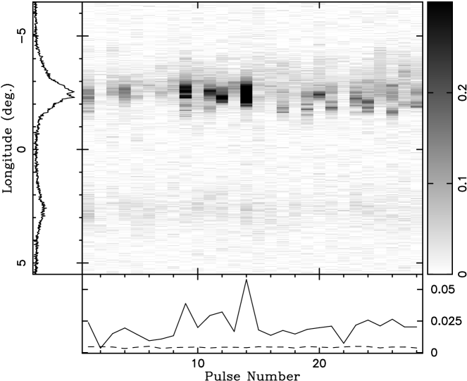
Figure 4: An example of the longitude-resolved modulation pattern (in grey-scale), obtained from 512 pulses folded at the putative carousel rotation period of $28.44P_{1}$, is shown in the main panel, with the associated integrated pulse profile on the left. Bottom plot shows the corresponding intensity-modulation pattern averaged over longitudes, clearly showing an evidence for periodic nulls. The dashed line represents the 4$\sigma$ detection threshold.

The periodic pseudo-nulls found by HR07 are among the best manifestations of the underlying carousel model responsible for the drifting subpulse phenomenon in pulsars. We have also checked our data for their presence, although given its erratic nature (Fig. 1) we were not very optimistic at first. However, to our surprise we managed to detect them in some selected, brighter pulse sequences. A good example from our results can be seen in Fig. 4, which shows the pattern of the modulation of the pulsar signal, folded with a period of $P_{4}=28.44P_{1}$ found by HR07. Each folding was performed over 512 pulses, i.e. about 18 putative periods $P_{4}$. In four of such foldings (out of 16), we found a clear evidence for periodic pseudo-nulls in the form of apparent “null zones” in the folded modulation pattern. One of our best examples, as shown in Fig. 4, can be compared with Fig. 7 in HR07. One could argue, that given the erratic nature of our data, such nulls can appear in our folded profiles by pure coincidence, as we do not detect the majority of the incoming pulses. But given the fact that we detect about 20% of pulses, the chance of appearance of such coincidental periodic genuine nulls (as opposed to periodic pseudo-nulls) is only $0.8^{18}=1.8$% (to minimize such chance occurrence we were forced on folding of a very long pulse sequences). Not to mention the fact that the folding procedure itself helps to detect pulses that individually remain just below our detection threshold. Indeed, during folding of 18 sequences, we improve our sensitivity by a factor of more than four ($\sqrt{18}$). Therefore, we believe that the detection of periodic pseudo-nulls in our 8.35 GHz data confirms directly the findings of HR07 at the much lower frequency of 327 MHz. At the same time, it ultimately proves the carousel model for PSR B1133+16, that is 23 subbeams completing one full circulation in exactly $28.44P_{1}$. It is worth emphasizing that we detected our pseudo-nulls at exactly this period, and the LFF in our best data sequences is also close to this value (Tables 1 and 2).

Summarizing, PSR B1133+16 seems to be a case of a pulsar that shows an organized behaviour of its individual pulses only for some limited-duration periods of time, and otherwise appears to be highly chaotic. We still do not know what triggers the switch from chaos to order, and we do not undrestand what is happening with the pulsar during the chaotic periods - this definitely requires further study. However, we seem to have enough evidence to claim that, when the order appears, the pulsar radiation can be explained by means of the rotating carousel model. Moreover, our results presented in this paper show that the most fundamental feature of the carousel model, that is the carousel circulation time ($P_{4}$) prevails despite various difficulties nature (in form of details and nuances of pulsar emission) puts in our way. Whether this is some aliasing-smeared drifting subpulse phenomenon observed at lower frequencies, or low flux density at high frequencies preventing the majority of individual pulses from reaching the detection threshold, the low frequency feature is often visible. Additionaly, one of the most representative features of the carousel model is the phenomenon of periodic pseudo-nulls, and it is very important to note that we detected them at exactly the value of $28.44P_{1}$ reported by HR07 at lower frequencies.

References

- Asgekar & Deshpande (2001) Asgekar A., Deshpande A.A., 2001, MNRAS, 326, 1249
- Asgekar & Deshpande (2005) Asgekar A., Deshpande A.A., 2005, MNRAS, 357, 1105
- Backer (1970) Backer D.C., 1970, Nature, 228, 1297
- Backer (1973) Backer D.C., 1973, ApJ, 182, 245
- DeLuca et al. (2005) De Luca A., Caraveo P.A., Mereghetti S., Negroni M. & Bignami G.F. 2005, ApJ, 623, 1051
- Deshpande & Rankin (1999) Deshpande A.A., Rankin J.M., 1999, ApJ, 524, 1008
- Deshpande & Rankin (2001) Deshpande A.A., Rankin J.M., 2001, MNRAS, 322, 438
- Drake & Craft (1968) Drake F.D., Craft H.D., 1968, Nature, 220, 231
- Gil, Melikidze & Geppert (2003) Gil J., Melikidze G., Geppert U., 2003, A&A, 407, 315
- Gil & Sendyk (2000) Gil J., Sendyk M., 2000, ApJ, 541, 351
- Gil & Sendyk (2003) Gil J., Sendyk M., 2003, ApJ, 585, 453