Systematic Low-Energy Effective Field Theory for Magnons and Holes in an Antiferromagnet on the Honeycomb Lattice

Abstract

Based on a symmetry analysis of the microscopic Hubbard and $t$-$J$ models, a systematic low-energy effective field theory is constructed for hole-doped antiferromagnets on the honeycomb lattice. In the antiferromagnetic phase, doped holes are massive due to the spontaneous breakdown of the $SU(2)_{s}$ symmetry, just as nucleons in QCD pick up their mass from spontaneous chiral symmetry breaking. In the broken phase the effective action contains a single-derivative term, similar to the Shraiman-Siggia term in the square lattice case. Interestingly, an accidental continuous spatial rotation symmetry arises at leading order. As an application of the effective field theory we consider one-magnon exchange between two holes and the formation of two-hole bound states. As an unambiguous prediction of the effective theory, the wave function for the ground state of two holes bound by magnon exchange exhibits $f$-wave symmetry.

1 Introduction

The physics of correlated electron systems is strongly influenced by the geometry of the underlying crystal lattice. For example, at weak coupling the half-filled Hubbard model on the honeycomb lattice is a semi-metal with massless fermion excitations residing in two Dirac cones. This situation is realized in graphene. At stronger coupling the $SU(2)_{s}$ symmetry breaks spontaneously and the system becomes an antiferromagnet, which may be realized in the dehydrated version of Na₂CoO${}_{2}\times y$H₂O. On a square lattice, on the other hand, due to Fermi surface nesting, the system is an antiferromagnet even at arbitrarily weak coupling. Upon doping, antiferromagnets on both the square and the honeycomb lattice may become high-temperature superconductors. Recenty, a spin-liquid phase was identified in numerical simulations between the free fermion graphene phase and the strongly correlated antiferromagnetic phase [1].

The low-energy physics of undoped antiferromagnets on a bipartite lattice is described by an $O(3)$-symmetric non-linear $\sigma$-model [2], whose systematic treatment is realized in magnon chiral perturbation theory [3, 4, 5, 6, 7, 8]. The effective theory for holes doped into an antiferromagnet on the square lattice was pioneered by Shraiman and Siggia [9]. In particular, these authors found an important term in the magnon-hole action known as the Shraiman-Siggia term. Based on the microscopic $t$-$J$ model, interesting results on magnon-mediated forces between holes were obtained in [10] and spiral phases were studied in [11, 12]. In analogy to baryon chiral perturbation theory for QCD [13, 14, 15, 16, 17], a systematic low-energy effective field theory for magnons and holes was constructed in [18, 19]. This theory has been used in a detailed analysis of two-hole states bound by one-magnon exchange [19, 20] as well as of spiral phases [21]. The systematic effective field theory investigations have also been extended to electron-doped antiferromagnets [22]. In that case, no Shraiman-Siggia-type term (with just a single spatial derivative) exists. Hence at low energies magnon-electron couplings are weaker than magnon-hole couplings. As a consequence, in contrast to hole-doped systems, in electron-doped systems there are no spiral phases with a helical structure in the staggered magnetization [22].

In this paper we construct a systematic low-energy effective field theory for hole-doped antiferromagnets on the honeycomb lattice. In the antiferromagnetic phase, the $SU(2)_{s}$ spin symmetry is spontaneously broken and the fermions pick up a mass. This is analogous to QCD where protons and neutrons pick up their masses due to spontaneous chiral symmetry breaking. Our analysis shows that the effective theory on the honeycomb lattice contains a term similar to the Shraiman-Siggia term in the square lattice case [9], which supports spiral phases. Remarkably, the leading terms of the effective theory have an accidental continuous rotation symmetry which is reduced to the discrete 60 degrees rotation symmetry $O$ of the microscopic honeycomb lattice only by the higher-order terms. While spiral phases in hole-doped antiferromagnets on the honeycomb lattice were explored in [23], here — as a further application of the effective field theory method — we derive the one-magnon exchange potentials between two holes and study the formation of two-hole bound states, which will turn out to have $f$-wave symmetry.

The rest of the paper is organized as follows. Section 2 contains a symmetry analysis of the underlying Hubbard and $t$-$J$ model. Section 3 is devoted to the low-energy effective theory for magnons — in particular, a non-linear realization of the $SU(2)_{s}$ spin symmetry is constructed. Based on the microscopic $t$-$J$ model, in Section 4, we include the holes in the effective field theory framework. In Section 5, one-magnon exchange potentials between two holes are derived and the resulting two-hole bound states are investigated in Section 6. Finally, section 7 contains our conclusions.

2 Microscopic Theory

We assume that the Hubbard model and the $t$-$J$-model are reliable models to describe doped quantum antiferromagnets, and therefore are valid as concrete microscopic models for the low-energy effective field theory for magnons and holes. Due to the fact that the effective Lagrangian to be constructed must inherit all symmetries of the underlying microscopic systems, a careful symmetry analysis of these microscopic models is presented in this section.

2.1 Symmetries of the Honeycomb Lattice

The honeycomb lattice is not a Bravais lattice — rather, it consists of two triangular Bravais sublattices A and B, as depicted in Figure 1.

Figure 1: Bipartite non-Bravais honeycomb lattice consisting of two triangular Bravais sublattices. The translation vectors are $a_{1}$ and $a_{2}$.

The primitive vectors that generate the triangular sublattices in coordinate space are given by

$$a_{1}=\sqrt{3}a\left(\frac{\sqrt{3}}{2},\frac{1}{2}\right),\ a_{2}=\sqrt{3}a\left(0,1\right),$$ (2.1)

where $a$ is the lattice spacing between two neighboring sites. The two basis vectors $b_{1}$ and $b_{2}$ that span the reciprocal lattice obey

$$a_{i}b_{j}=2\pi\delta_{ij},$$ (2.2)

and are given by

$$b_{1}=\frac{4\pi}{3a}\left(1,0\right),\ b_{2}=\frac{4\pi}{3a}\left(-\frac{1}{2},\frac{\sqrt{3}}{2}\right).$$ (2.3)

The vectors $b_{1}$ and $b_{2}$ generate the hexagonal first Brillouin zone of the triangular lattice. Since the honeycomb lattice consists of two triangular sublattices, its momentum space is doubly-covered.

The honeycomb lattice exhibits a number of discrete symmetries. Translations by the vectors $a_{i}$ are denoted by $D_{i}$. Counter-clockwise rotations by 60 degrees around the center of a hexagon are denoted by $O$, and reflections at the $x_{1}$-axis going through the center of the hexagon are denoted by $R$. Translations by other distance vectors, rotations by other angles or around other centers, and reflections with respect to other axes can be obtained as combinations of the elementary symmetry operations $D_{1}$, $D_{2}$, $O$, and $R$.

2.2 Symmetries of the Hubbard Model

Let $c_{xs}^{\dagger}$ denote the operator which creates a fermion with spin $s\in\{\uparrow,\downarrow\}$ on a lattice site $x=(x_{1},x_{2})$. The corresponding annihilation operator is $c_{xs}$. These fermion operators obey the canonical anticommutation relations

$$\{c_{xs}^{\dagger},c_{ys^{\prime}}\}=\delta_{xy}\delta_{ss^{\prime}},\ \{c_{xs},c_{ys^{\prime}}\}=\{c_{xs}^{\dagger},c_{ys^{\prime}}^{\dagger}\}=0.$$ (2.4)

The second quantized Hubbard Hamiltonian is defined by

$$H=-t\sum_{\genfrac{}{}{0.0pt}{}{\langle x,y\rangle}{s=\uparrow,\downarrow}}(c_{xs}^{\dagger}c_{ys}+c_{ys}^{\dagger}c_{xs})+U\sum_{x}c_{x\uparrow}^{\dagger}c_{x\uparrow}c_{x\downarrow}^{\dagger}c_{x\downarrow}-\mu^{\prime}\sum_{\genfrac{}{}{0.0pt}{}{x}{s=\uparrow,\downarrow}}c_{xs}^{\dagger}c_{xs},$$ (2.5)

where $\langle x,y\rangle$ indicates summation over nearest neighbors, $t$ is the hopping parameter, and the parameter $U>0$ fixes the strength of the Coulomb repulsion between two fermions located on the same lattice site. The parameter $\mu^{\prime}$ denotes the chemical potential.

The fermion creation and annihilation operators can be used to define the following $SU(2)_{s}$ Pauli spinors

$$c_{x}^{\dagger}=\left(c_{x\uparrow}^{\dagger},c_{x\downarrow}^{\dagger}\right),\qquad c_{x}=\left(\begin{array}[]{c}c_{x\uparrow}\\ c_{x\downarrow}\end{array}\right).$$ (2.6)

In terms of these operators, the Hubbard model can be reformulated as

$$H=-t\sum_{\langle xy\rangle}(c_{x}^{\dagger}c_{y}+c_{y}^{\dagger}c_{x})+\frac{U}{2}\sum_{x}(c_{x}^{\dagger}c_{x}-1)^{2}-\mu\sum_{x}(c_{x}^{\dagger}c_{x}-1).$$ (2.7)

The parameter $\mu=\mu^{\prime}-\frac{U}{2}$ controls doping where the fermions are counted with respect to half-filling.

Since all terms in the effective Lagrangian must be invariant under all symmetries of the Hubbard model, a careful symmetry analysis of Eq.(2.7) is needed. Let us divide the symmetries of the Hubbard model into two categories: Continuous symmetries ($SU(2)_{s}$, $U(1)_{Q}$ fermion number and its non-Abelian extension $SU(2)_{Q}$), which are internal symmetries of Eq.(2.7), and discrete symmetries ($D_{i}$, $O$ and $R$), which are symmetry transformations of the underlying honeycomb lattice. There is also time reversal which is implemented by an anti-unitary operator $T$. This symmetry will be discussed further in the effective field theory framework.

In order to construct the appropriate unitary transformation representing a global $SU(2)_{s}$ spin rotation, we first define the total $SU(2)_{s}$ spin operator by

$$\vec{S}=\sum_{x}\vec{S}_{x}=\sum_{x}c_{x}^{\dagger}\ \frac{\vec{\sigma}}{2}\ c_{x}.$$ (2.8)

The spin symmetry is implemented by the unitary operator

$$V=\exp(i\vec{\eta}\cdot\vec{S}),$$ (2.9)

which acts on $c_{x}$ as

$$c_{x}^{\prime}=V^{\dagger}c_{x}V=\exp(i\vec{\eta}\cdot\frac{\vec{\sigma}}{2})c_{x}=gc_{x},\qquad g\in SU(2)_{s}.$$ (2.10)

The total spin is conserved and the Hubbard Hamiltonian is invariant under global $SU(2)_{s}$ spin rotations. This symmetry, however, is spontaneously broken: the corresponding order parameter is the staggered magnetization vector

$$\vec{M}_{s}=\sum_{x}(-1)^{x}\vec{S}_{x},$$ (2.11)

which takes a non-zero expectation value in the ground state of the antiferromagnet. We define $(-1)^{x}=1$ for all $x\in A$ and $(-1)^{x}=-1$ for all $x\in B$, where $A$ and $B$ are the two triangular sublattices of the honeycomb lattice.

The unitary transformation of the $U(1)_{Q}$ symmetry involves the charge operator

$$Q=\sum_{x}Q_{x}=\sum_{x}(c_{x}^{\dagger}c_{x}-1)=\sum_{x}(c_{x\uparrow}^{\dagger}c_{x\uparrow}+c_{x\downarrow}^{\dagger}c_{x\downarrow}-1),$$ (2.12)

which counts the fermion number with respect to half-filling. The corresponding unitary operator is given by

$$W=\exp(i\omega Q),$$ (2.13)

and the fermion operators transform as

$$^{Q}c_{x}=W^{\dagger}c_{x}W=\exp(i\omega)c_{x},\qquad\exp(i\omega)\in U(1)_{Q}.$$ (2.14)

Charge or fermion number are conserved due to $[H,Q]=0$.

The Hubbard model shows invariance under shifts along the two primitive lattice vectors $a_{1}$ and $a_{2}$. These transformations are generated by the unitary operators $D_{i}$, which act on the spinor $c_{x}$ as

$$^{D_{i}}c_{x}=D^{\dagger}_{i}c_{x}D_{i}=c_{x+a_{i}}.$$ (2.15)

By applying Eq.(2.15) on the Hubbard Hamiltonian of Eq.(2.7) and redefining the sum over lattice sites $x$, one can see that indeed $[H,D_{i}]=0$. Since the shift symmetry maps $A\rightarrow A$ and $B\rightarrow B$, this transformation does not affect the order parameter $\vec{M}_{s}$.

A spatial rotation by 60 degrees leaves Eq.(2.7) invariant. Since spin-orbit coupling is neglected in the Hubbard model, spin decouples from the spatial motion and becomes an internal quantum number. The rotation symmetry is implemented by the use of a unitary operator $O$, which acts on the fermion operators as

$$^{O}c_{x}=O^{\dagger}c_{x}O=c_{Ox}.$$ (2.16)

Rotation symmetry on the honeycomb lattice is spontaneously broken because $O$ exchanges the two sublattices $A\leftrightarrow B$ and therefore the staggered magnetization $\vec{M}_{s}$ gets flipped. This is, however, just the same as redefining the sign of $(-1)^{x}$ and does therefore not change the physics. In the construction of the effective field theory for magnons and holes, it will turn out to be useful to also consider the combined symmetry $O^{\prime}$ consisting of a spatial rotation $O$ and a global $SU(2)_{s}$ spin rotation $g=i\sigma_{2}$. $O^{\prime}$ transforms $c_{x}$ as

$$^{O^{\prime}}c_{x}=O^{{}^{\prime}\dagger}c_{x}O^{\prime}=(i\sigma_{2})\,^{O}c_{x}=(i\sigma_{2})c_{Ox}.$$ (2.17)

The specific $SU(2)_{s}$ element $g=i\sigma_{2}$ corresponds to a global spin rotation by 180 degrees and thus flips back $\vec{M}_{s}$, such that, in fact, at the end the order parameter is not affected by $O^{\prime}$. As opposed to the honeycomb lattice case, $\vec{M}_{s}$ changes sign under the shift symmetry $D_{i}$ on a bipartite square lattice [18]. In this case, a combined shift symmetry $D^{\prime}_{i}$ leaves the ground state invariant. Since on the square lattice a 90 degrees rotation $O$ maps sublattices $A\rightarrow A$ and $B\rightarrow B$, in that case the ground state is not affected by a rotation by an angle of 90 degrees.

Finally, the Hubbard Hamiltonian is invariant under the reflection $R$ at the $x_{1}$-axis shown in Figure 1. Under this transformation, the fermion operators transform as

$$^{R}c_{x}=R^{\dagger}c_{x}R=c_{Rx}.$$ (2.18)

Since $R$ maps the two sublattices onto themselves, $\vec{M}_{s}$ remains invariant.

In [24, 25], Yang and Zhang proved the existence of a non-Abelian extension of the $U(1)_{Q}$ fermion number symmetry in the half-filled Hubbard model. This pseudospin symmetry contains $U(1)_{Q}$ as a subgroup. The $SU(2)_{Q}$ symmetry is realized on the square as well as on the honeycomb lattice and is generated by the three operators

$$Q^{+} =\sum_{x}(-1)^{x}c_{x\uparrow}^{\dagger}c_{x\downarrow}^{\dagger},\qquad Q^{-}=\sum_{x}(-1)^{x}c_{x\downarrow}c_{x\uparrow},$$

$$Q^{3} =\sum_{x}\frac{1}{2}(c_{x\uparrow}^{\dagger}c_{x\uparrow}+c_{x\downarrow}^{\dagger}c_{x\downarrow}-1)=\frac{1}{2}Q.$$ (2.19)

The factor $(-1)^{x}$ again distinguishes between the two sublattices $A$ and $B$ of the honeycomb lattice. Defining $Q^{1}$ and $Q^{2}$ through $Q^{\pm}=Q^{1}\pm iQ^{2}$, one readily shows that the $SU(2)_{Q}$ Lie-algebra $[Q^{a},Q^{b}]=i\varepsilon_{abc}Q^{c}$, with $a,b,c\in\{1,2,3\}$, indeed is satisfied and that $[H,\vec{Q}]=0$ with $\vec{Q}=(Q^{1},Q^{2},Q^{3})$ for the Hubbard Hamiltonian with $\mu=0$.

In order to write the Hubbard Hamiltonian Eq.(2.5) or Eq.(2.7) in a manifestly invariant form under $SU(2)_{s}\times SU(2)_{Q}$, we arrange the fermion operators in a $2\times 2$ matrix-valued operator, arriving at the fermion representation

$$C_{x}=\left(\begin{array}[]{cc}c_{x\uparrow}&(-1)^{x}\ c^{\dagger}_{x\downarrow}\\ c_{x\downarrow}&-(-1)^{x}c_{x\uparrow}^{\dagger}\end{array}\right).$$ (2.20)

The $SU(2)_{Q}$ transformation behavior of Eq.(2.20) can now be worked out by applying the unitary operator $W=\exp(i\vec{\omega}\cdot\vec{Q})$,

$${}^{\vec{Q}}C_{x}=W^{\dagger}C_{x}W=C_{x}\Omega^{T},$$ (2.21)

with

$$\Omega=\exp\left(i\vec{\omega}\cdot\frac{\vec{\sigma}}{2}\right)\in SU(2)_{Q}.$$ (2.22)

Under an $SU(2)_{s}$ spin rotation, $C_{x}$ transforms exactly like $c_{x}$, i.e.

$$C_{x}^{\prime}=gC_{x},\qquad g\in SU(2)_{s}.$$ (2.23)

Applying an $SU(2)_{s}\times SU(2)_{Q}$ transformation to Eq.(2.20) then leads to

$$^{\vec{Q}}C_{x}^{\prime}=gC_{x}\Omega^{T}.$$ (2.24)

Since the $SU(2)_{s}$ spin symmetry acts from the left and the $SU(2)_{Q}$ pseudospin symmetry acts from the right onto the fermion operator, it is now obvious that these two non-Abelian symmetries commute with each other. Under the discrete symmetries of the Hubbard model, $C_{x}$ has the following transformation properties

$$D_{i}: {}^{D_{i}}C_{x} =C_{x+a_{i}},$$

$$O: {}^{O}C_{x} =C_{Ox}\sigma_{3},$$

$$O^{\prime}: {}^{O^{\prime}}C_{x} =\left(i\sigma_{2}\right)C_{Ox}\sigma_{3},$$

$$R: {}^{R}C_{x} =C_{Rx}.$$ (2.25)

In terms of Eq.(2.20), we are now able to write down the Hubbard Hamiltonian in the manifestly $SU(2)_{s}$, $U(1)_{Q}$, $D_{i}$, $O$, $O^{\prime}$ and $R$ invariant form

$$H=-\frac{t}{2}\sum_{\langle xy\rangle}\mbox{Tr}[C_{x}^{\dagger}C_{y}+C_{y}^{\dagger}C_{x}]+\frac{U}{12}\sum_{x}\mbox{Tr}[C_{x}^{\dagger}C_{x}C_{x}^{\dagger}C_{x}]-\frac{\mu}{2}\sum_{x}\mbox{Tr}[C_{x}^{\dagger}C_{x}\sigma_{3}].$$ (2.26)

The $\sigma_{3}$ Pauli matrix in the chemical potential term prevents the Hubbard Hamiltonian from being invariant under $SU(2)_{Q}$ away from half-filling. For $\mu\neq 0$, $SU(2)_{Q}$ is explicitly broken to its subgroup $U(1)_{Q}$. In addition, the pseudospin symmetry is realized in Eq.(2.26) only for nearest-neighbor hopping. As soon as next-to-nearest-neighbor hopping is included, the $SU(2)_{Q}$ invariance gets lost even for $\mu=0$. The continuous $SU(2)_{Q}$ symmetry contains a discrete particle-hole symmetry. Although this pseudospin symmetry is not present in real materials, it will play an important role in the construction of the effective field theory. The identification of the final effective fields for holes will lead us to explicitly break the $SU(2)_{Q}$ symmetry in Section 4.

2.3 Symmetries of the $t$-$J$ Model

Away from half-filling and for $U\gg t$, the Hubbard model reduces to the $t$-$J$ model, which is defined by the Hamiltonian

$$H=\mathcal{P}\bigg{\{}-t\sum_{\langle xy\rangle}(c_{x}^{\dagger}c_{y}+c_{y}^{\dagger}c_{x})+J\sum_{\langle xy\rangle}\vec{S}_{x}\cdot\vec{S}_{y}-\mu\sum_{x}(c_{x}^{\dagger}c_{x}-1)\bigg{\}}\mathcal{P}.$$ (2.27)

Using second order perturbation theory, the antiferromagnetic exchange coupling $J$ is related to the parameters of the Hubbard model by $J=\frac{2t^{2}}{U}>0$. Again, $t$ is the hopping amplitude, $\vec{S}_{x}$ is the $SU(2)_{s}$ spin operator on a site $x$, and $\mu$ controls the doping with respect to a half-filled system. The projection operator $\mathcal{P}$ removes all doubly occupied sites from the Hilbert space and hence the $t$-$J$ model can only be doped with holes. In [26], the single-hole sector of the $t$-$J$ model was simulated on the honeycomb lattice by using an efficient loop-cluster algorithm. For the construction of the effective theory for a hole doped antiferromagnet, the $t$-$J$ model will serve as the microscopic starting point. Except for the $SU(2)_{Q}$ symmetry, this model shares all symmetries with the more general Hubbard model.

3 Effective Theory for Magnons

In this section we investigate the low-energy physics of an undoped quantum antiferromagnet. We will first argue that quantum antiferromagnets are systems featuring a spontaneous $SU(2)_{s}\to U(1)_{s}$ symmetry breakdown, which induces two massless Goldstone bosons — the magnons. We present the leading-order effective action for the pure magnon sector of an antiferromagnet on the honeycomb lattice. In addition, a non-linear realization of the spontaneously broken $SU(2)_{s}$ spin symmetry is constructed, which will enable us to couple magnons and doped holes in section 4.

3.1 Low-Energy Effective Action for Magnons

In quantum antiferromagnets the symmetry group $G=SU(2)_{s}$ of global spin rotations is spontaneously broken by the formation of a staggered magnetization. The ground state of these systems is invariant only under spin rotations in the subgroup $H=U(1)_{s}$. As a consequence of the spontaneous global symmetry breaking, there are two magnons which are described by a unit-vector field

$$\vec{e}(x)=\big{(}e_{1}(x),e_{2}(x),e_{3}(x)\big{)}\in S^{2},\qquad\vec{e}(x)^{2}=1,$$ (3.1)

in the coset space $G/H=SU(2)_{s}/U(1)_{s}=S^{2}$. Here $x=(x_{1},x_{2},t)$ denotes a point in Euclidean space-time. The low-energy physics of an undoped antiferromagnet can be completely described in terms of the field $\vec{e}(x)$ which represents the direction of the local staggered magnetization.

Later, we will couple magnons to holes. Since holes have spin 1/2 and are thus described by two-component fields, it is convenient to work with a $\mathbb{C}P(1)$ representation instead of the $O(3)$ vector representation for the magnon field. We introduce the $2\times 2$ Hermitean projection matrices $P(x)$ defined by

$$P(x)=\frac{1}{2}\big{[}\mathbbm{1}+\vec{e}(x)\cdot\vec{\sigma}\big{]}=\frac{1}{2}\left(\begin{array}[]{cc}1+e_{3}(x)&e_{1}(x)-ie_{2}(x)\\ e_{1}(x)+ie_{2}(x)&1-e_{3}(x)\end{array}\right),$$ (3.2)

obeying

$$P(x)^{\dagger}=P(x),\qquad\mbox{Tr}P(x)=1,\qquad P(x)^{2}=P(x).$$ (3.3)

In terms of $P(x)$, to lowest-order in a systematic derivative expansion, the effective action for magnons is given by

$$S[P]=\int d^{2}\!x\,dt\ \rho_{s}\mbox{Tr}[\partial_{i}P\partial_{i}P+\frac{1}{c^{2}}\partial_{t}P\partial_{t}P].$$ (3.4)

Here we have introduced two low-energy constants, the spin stiffness $\rho_{s}$ and the spinwave velocity $c$. The values of these low-energy constants have been determined very precisely using Monte Carlo simulations [27, 28, 29]. It should be pointed out that this leading-order contribution to the effective action is exactly the same as for an antiferromagnet on a square lattice. Deviations will only show up when higher order terms with more derivatives are considered.

We now discuss how the magnon field $P(x)$ transforms under the various symmetries of the underlying microscopic models. Under global $SU(2)_{s}$ spin transformations the staggered magnetization field transforms as

$$P(x)^{\prime}=gP(x)g^{\dagger}.$$ (3.5)

Note that it is invariant under the Abelian and the non-Abelian fermion number symmetries $U(1)_{Q}$ and $SU(2)_{Q}$, i.e.

$${}^{\vec{Q}}P(x)=P(x).$$ (3.6)

Under the displacement $D_{i}$ and the reflection symmetry $R$, the sublattices are not interchanged such that

$${}^{D_{i}}P(x) =P(x),$$

$${}^{R}P(x) =P(Rx).$$ (3.7)

Under a rotation by 60 degrees, the staggered magnetization vector changes sign, i.e. ${}^{O}\vec{e}(x)=-\vec{e}(Ox)$, and therefore

$$^{O}P(x)=\frac{1}{2}\big{[}\mathbbm{1}-\vec{e}(Ox)\cdot\vec{\sigma}\big{]}=\mathbbm{1}-P(Ox).$$ (3.8)

Note that in an antiferromagnet on the honeycomb lattice the 60 degrees rotation symmetry is spontaneously broken, whereas in an antiferromagnet on the square lattice, it is the displacement symmetry by one lattice spacing which is spontaneously broken. The above transformation property simplifies under the composed symmetry $O^{\prime}$,

$$^{O^{\prime}}P(x)=(i\sigma_{2})\,^{O}P(x)(i\sigma_{2})^{\dagger}=P(Ox)^{*}.$$ (3.9)

Under time-reversal $T$, which turns a space-time point $x=(x_{1},x_{2},t)$ into $Tx=(x_{1},x_{2},-t)$, the staggered magnetization changes sign and, as a consequence,

$${}^{T}P(x)=\mathbbm{1}-P(Tx).$$ (3.10)

Since also $T$ is a spontaneously broken symmetry, again it is useful to consider the composed transformation $T^{\prime}$ consisting of a regular time-reversal $T$ and the specific spin rotation $g=i\sigma_{2}$. Under the unbroken symmetry $T^{\prime}$ the magnon field $P(x)$ transforms as

$${}^{T^{\prime}}P(x)=(i\sigma_{2})^{T}P(x)(i\sigma_{2})^{\dagger}=P(Tx)^{*}.$$ (3.11)

The effective action in Eq.(3.4) is invariant under all these symmetries.

3.2 Non-linear Realization of the $SU(2)_{s}$ Symmetry

In order to couple the fermions to the magnons, i.e. to the antiferromagnetic order parameter, a non-linear realization of the $SU(2)_{s}$ symmetry has been constructed and discussed in detail in [18]. The spin symmetry is implemented on the fermion fields by a non-linear local transformation $h(x)\in U(1)_{s}$. This local transformation is constructed from the global transformation $g\in SU(2)_{s}$ and the magnon field $P(x)$ as follows. One first defines a local, unitary transformation $u(x)\in SU(2)_{s}$ which diagonalizes the staggered magnetization field, i.e.

$$u(x)P(x)u(x)^{\dagger}=\frac{1}{2}({\mathbbm{1}}+\sigma_{3})=\left(\begin{array}[]{cc}1&0\\ 0&0\end{array}\right),\qquad u_{11}(x)\geq 0.$$ (3.12)

In order to make $u(x)$ uniquely defined, we demand that the element $u_{11}(x)$ is real and non-negative. Using Eq.(3.2) and spherical coordinates for $\vec{e}(x)$, i.e.

$$\vec{e}(x)=\big{(}\sin\theta(x)\cos\varphi(x),\sin\theta(x)\sin\varphi(x),\cos\theta(x)\big{)},$$ (3.13)

one obtains [18]

$$u(x) =\frac{1}{\sqrt{2(1+e_{3}(x))}}\left(\begin{array}[]{cc}1+e_{3}(x)&e_{1}(x)-ie_{2}(x)\\ -e_{1}(x)-ie_{2}(x)&1+e_{3}(x)\end{array}\right)$$ (3.16)

$$=\left(\begin{array}[]{cc}\cos\left(\frac{\theta(x)}{2}\right)&\sin\left(\frac{\theta(x)}{2}\right)\exp(-i\varphi(x))\\[2.15277pt] -\sin\left(\frac{\theta(x)}{2}\right)\exp(i\varphi(x))&\cos\left(\frac{\theta(x)}{2}\right)\end{array}\right).$$ (3.19)

Note that the local transformation $u(x)$ rotates an arbitrary staggered magnetization field configuration $P(x)$ into the specific constant diagonal field configuration with $P(x)=\frac{1}{2}({\mathbbm{1}}+\sigma_{3})$. Under a global $SU(2)_{s}$ transformation $g$ the diagonalizing field $u(x)$ transforms as

$$u(x)^{\prime}=h(x)u(x)g^{\dagger},\qquad u_{11}(x)^{\prime}\geq 0,$$ (3.20)

which implicitly defines the non-linear symmetry transformation

$$h(x)=\exp\big{(}i\alpha(x)\sigma_{3}\big{)}=\left(\begin{array}[]{cc}\exp(i\alpha(x))&0\\ 0&\exp(-i\alpha(x))\end{array}\right)\in U(1)_{s}.$$ (3.21)

The transformation $h(x)$ is uniquely defined since we demand that $u_{11}(x)^{\prime}$ is again real and non-negative.

The transformation behavior of the field $u(x)$ can be easily worked out from the known transformation behavior of $P(x)$. Since $u(x)$ contains only magnon degrees of freedom, it transforms trivially under both the Abelian and the non-Abelian fermion number symmetries $U(1)_{Q}$ and $SU(2)_{Q}$, i.e.

$${}^{\vec{Q}}u(x)=u(x).$$ (3.22)

Under the displacement $D_{i}$ and the reflection symmetry $R$ one finds

$${}^{D_{i}}u(x) =u(x),$$

$${}^{R}u(x) =u(Rx).$$ (3.23)

The spontaneous breaking of the 60 degrees rotation symmetry $O$ which takes $\vec{e}(x)$ to $-\vec{e}(Ox)$ leads to

$${}^{O}u(x)=\tau(Ox)u(Ox),$$ (3.24)

with

$$\tau(x) =\frac{1}{\sqrt{e_{1}(x)^{2}+e_{2}(x)^{2}}}\left(\begin{array}[]{cc}0&-e_{1}(x)+ie_{2}(x)\\ e_{1}(x)+ie_{2}(x)&0\end{array}\right)$$ (3.27)

$$=\left(\begin{array}[]{cc}0&-\exp(-i\varphi(x))\\ \exp(i\varphi(x))&0\end{array}\right).$$ (3.30)

Under the combined symmetry $O^{\prime}$ one finds

$$^{O^{\prime}}u(x)=u(Ox)^{*}.$$ (3.31)

Since time-reversal $T$ is a spontaneously broken discrete symmetry in an antiferromagnet, it acts on $u(x)$ as

$${}^{T}u(x)=\tau(Tx)u(Tx).$$ (3.32)

On the other hand, the combined time-reversal $T^{\prime}$ is unbroken and therefore realized in a linear manner, i.e.

$${}^{T^{\prime}}u(x)=u(Tx)^{*}.$$ (3.33)

Finally, we introduce the composite magnon fields $v_{\mu}(x)$ whose components will be used to couple the magnons to the fermions. Using the diagonalizing field $u(x)$, we define the composite magnon field

$$v_{\mu}(x)=u(x)\partial_{\mu}u(x)^{\dagger},$$ (3.34)

which under $SU(2)_{s}$ transforms as

$$v_{\mu}(x)^{\prime}=h(x)u(x)g^{\dagger}\partial_{\mu}[gu(x)^{\dagger}h(x)^{\dagger}]=h(x)[v_{\mu}(x)+\partial_{\mu}]h(x)^{\dagger}.$$ (3.35)

Since the field $v_{\mu}(x)$ is traceless and anti-Hermitean, it can be written as a linear combination of the Pauli matrices $\sigma_{a}$,

$$v_{\mu}(x)=iv_{\mu}^{a}(x)\sigma_{a},\qquad a\in\{1,2,3\},\qquad v_{\mu}^{a}(x)\in\mathbbm{R}.$$ (3.36)

Introducing

$$v_{\mu}^{\pm}(x)=v_{\mu}^{1}(x)\mp iv_{\mu}^{2}(x),$$ (3.37)

we arrive at

$$v_{\mu}(x)=i\left(\begin{array}[]{cc}v_{\mu}^{3}(x)&v_{\mu}^{+}(x)\\ v_{\mu}^{-}(x)&-v_{\mu}^{3}(x)\end{array}\right).$$ (3.38)

Under global $SU(2)_{s}$ transformations the components of $v_{\mu}$ transform as

$$v_{\mu}^{3}(x)^{\prime} = v_{\mu}^{3}(x)-\partial_{\mu}\alpha(x),$$

$$v_{\mu}^{\pm}(x)^{\prime} = \exp(\pm 2i\alpha(x))v_{\mu}^{\pm}(x),$$ (3.39)

which indicates that $v_{\mu}^{3}$ behaves like an Abelian $U(1)_{s}$ gauge field, while $v^{\pm}_{\mu}(x)$ exhibit the behavior of vector fields “charged” under $U(1)_{s}$. The transformation properties of the components $v_{\mu}^{3}(x)$ and $v^{\pm}_{\mu}(x)$ under the discrete symmetries can be worked out from the definition of $v_{\mu}(x)$ in Eq.(3.34) as well, and are summarized as follows

$$D_{i}: {}^{D_{i}}v_{\mu}^{3}(x) =v_{\mu}^{3}(x),$$

$$O: {}^{O}v_{1}^{3}(x) =\tfrac{1}{2}\big{[}-v_{1}^{3}(Ox)+\partial_{1}\varphi(Ox)-\sqrt{3}v_{2}^{3}(Ox)+\sqrt{3}\partial_{2}\varphi(Ox)\big{]},$$

$${}^{O}v_{2}^{3}(x) =\tfrac{1}{2}\big{[}\sqrt{3}v_{1}^{3}(Ox)-\sqrt{3}\partial_{1}\varphi(Ox)-v_{2}^{3}(Ox)+\partial_{2}\varphi(Ox)\big{]},$$

$${}^{O}v_{t}^{3}(x) =-v_{t}^{3}(Ox)+\partial_{t}\varphi(Ox),$$

$$O^{\prime}: {}^{O^{\prime}}v_{1}^{3}(x) =-\tfrac{1}{2}\big{[}v_{1}^{3}(Ox)+\sqrt{3}v_{2}^{3}(Ox)\big{]},$$

$${}^{O^{\prime}}v_{2}^{3}(x) =\tfrac{1}{2}\big{[}\sqrt{3}v_{1}^{3}(Ox)-v_{2}^{3}(Ox)\big{]},$$

$${}^{O^{\prime}}v_{t}^{3}(x) =-v_{t}^{3}(Ox),$$

$$R :\quad {}^{R}v_{1}^{3}(x) =v_{1}^{3}(Rx),$$

$${}^{R}v_{2}^{3}(x) =-v_{2}^{3}(Rx),$$

$${}^{R}v_{t}^{3}(x) =v_{t}^{3}(Rx),$$

$$T :\quad {}^{T}v_{i}^{3}(x) =-v_{i}^{3}(Tx)+\partial_{i}\varphi(Tx),$$

$${}^{T}v_{t}^{3}(x) =v_{t}^{3}(Tx)-\partial_{t}\varphi(Tx),$$

$$T^{\prime} :\quad {}^{T^{\prime}}v_{i}^{3}(x) =-v_{i}^{3}(Tx),$$

$${}^{T^{\prime}}v_{t}^{3}(x) =v_{t}^{3}(Tx),$$ (3.40)

and

$$D_{i}: {}^{D_{i}}v_{\mu}^{\pm}(x) =v_{\mu}^{\pm}(x),$$

$$O: {}^{O}v_{1}^{\pm}(x) =-\exp(\mp 2i\varphi(Ox))\tfrac{1}{2}\big{(}v_{1}^{\mp}(Ox)+\sqrt{3}v_{2}^{\mp}(Ox)\big{)},$$

$${}^{O}v_{2}^{\pm}(x) =\exp(\mp 2i\varphi(Ox))\tfrac{1}{2}\big{(}\sqrt{3}v_{1}^{\mp}(Ox)-v_{2}^{\mp}(Ox)\big{)},$$

$${}^{O}v_{t}^{\pm}(x) =-\exp(\mp 2i\varphi(Ox))v_{t}^{\mp}(x),$$

$$O^{\prime}: {}^{O^{\prime}}v_{1}^{\pm}(x) =-\tfrac{1}{2}\big{(}v_{1}^{\mp}(Ox)+\sqrt{3}v_{2}^{\mp}(Ox)\big{)},$$

$${}^{O^{\prime}}v_{2}^{\pm}(x) =\tfrac{1}{2}\big{(}\sqrt{3}v_{1}^{\mp}(Ox)-v_{2}^{\mp}(Ox)\big{)},$$

$${}^{O^{\prime}}v_{t}^{\pm}(x) =-v_{t}^{\mp}(Ox),$$

$$R :\quad {}^{R}v_{1}^{\pm}(x) =v_{1}^{\pm}(Rx),$$

$${}^{R}v_{2}^{\pm}(x) =-v_{2}^{\pm}(Rx),$$

$${}^{R}v_{t}^{\pm}(x) =v_{t}^{\pm}(Rx),$$

$$T :\quad {}^{T}v_{i}^{\pm}(x) =-\exp(\mp 2i\varphi(Tx))v_{i}^{\mp}(Tx),$$

$${}^{T}v_{t}^{\pm}(x) =\exp(\mp 2i\varphi(Tx))v_{t}^{\mp}(Tx),$$

$$T^{\prime} :\quad {}^{T^{\prime}}v_{i}^{\pm}(x) =-v_{i}^{\mp}(Tx),$$

$${}^{T^{\prime}}v_{t}^{\pm}(x) =v_{t}^{\mp}(Tx).$$ (3.41)

The magnon action of Eq.(3.4) can now be reformulated in terms of the composite magnon field $v_{\mu}(x)$,

$$S[v_{\mu}^{\pm}]=\int d^{2}\!x\,dt\ 2\rho_{s}\left(v^{+}_{i}v^{-}_{i}+\frac{1}{c^{2}}v_{t}^{+}v_{t}^{-}\right).$$ (3.42)

At a first glance, the expression $v_{\mu}^{+}v_{\mu}^{-}$ looks like a mass term of a charged vector field. However, since it contains derivatives acting on $u(x)$, it is just the kinetic term of a massless Goldstone boson.

4 Effective Theory for Magnons and Holes

In this section we construct a systematic low-energy effective theory for holes coupled to magnons. As a first step toward building the effective theory, we identify the correct low-energy degrees of freedom that describe the holes. Then the transformation behavior of these fermionic fields is investigated in great detail. Finally, the most general effective Lagrangian for magnons and holes is constructed.

4.1 Fermion Fields and their Transformation Properties

In order to construct the effective theory for hole-doped antiferromagnets, it is essential to know where the hole pockets are located in momentum space. The dispersion relation $E(k)$ for a single hole in the $t$-$J$ model on the honeycomb lattice was simulated using an efficient loop-cluster algorithm [26]. The result is shown in Figure 2.

Figure 2: The dispersion relation $E(k)/t$ for a single hole in an antiferromagnet on the honeycomb lattice simulated in the $t$-$J$ model for $J/t=2$ [26].

This simulation clearly shows spherically shaped hole pockets centered around $(\pm\frac{2\pi}{3a},\pm\frac{2\pi}{3\sqrt{3}a})$ and $(0,\pm\frac{4\pi}{3\sqrt{3}a})$ in the first Brillouin zone. Therefore, doped holes occupy the two pockets $\alpha$ and $\beta$ with lattice momenta

$$k^{\alpha}=-k^{\beta}=(0,\frac{4\pi}{3\sqrt{3}a}).$$ (4.1)

Together with the origin, these two points form a minimal set of three points in momentum space. The three points in coordinate space that are related to $0,k^{\alpha},k^{\beta}$ by a discrete Fourier transform, define three triangular sublattices $A_{1}$, $A_{2}$, and $A_{3}$, as well as $B_{1}$, $B_{2}$, and $B_{3}$ on the $A$- and $B$-sublattices of the honeycomb lattice. The geometry of these six triangular sublattices is illustrated in Figure 3.

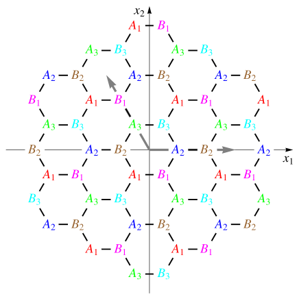
Figure 3: $\{A_{1},A_{2},A_{3}\}$ and $\{B_{1},B_{2},B_{3}\}$ sublattice structure and the corresponding primitive lattice vectors.

We now introduce fermionic lattice operators with a sublattice index $X$ as an intermediate step between the microscopic and the effective fermion fields,

$$\Psi^{X}_{x}=u(x)C_{x},$$ (4.2)

with $x\in X$, $X\in\{A_{1},A_{2},A_{3},B_{1},B_{2},B_{3}\}$. The above definition of $\Psi^{X}_{x}$ contains the diagonalizing matrix $u(x)$ of Eq.(3.16) and hence accounts for the non-linearly realized $SU(2)_{s}$ symmetry on the effective fermion fields. On even and odd sublattices the fermion operator has the following components

$$\Psi^{X}_{x}=u(x)\begin{pmatrix}c_{x\uparrow}&c_{x\downarrow}^{\dagger}\\ c_{x\downarrow}&-c_{x\uparrow}^{\dagger}\end{pmatrix}=\begin{pmatrix}\psi^{X}_{x,+}&\psi^{X^{\dagger}}_{x,-}\\ \psi^{X}_{x,-}&-\psi^{X^{\dagger}}_{x,+}\end{pmatrix},\quad x\in X,X\in\{A_{1},A_{2},A_{3}\},$$ (4.3)

and

$$\Psi^{X}_{x}=u(x)\begin{pmatrix}c_{x\uparrow}&-c_{x\downarrow}^{\dagger}\\ c_{x\downarrow}&c_{x\uparrow}^{\dagger}\end{pmatrix}=\begin{pmatrix}\psi^{X}_{x,+}&-\psi^{X^{\dagger}}_{x,-}\\ \psi^{X}_{x,-}&\psi^{X^{\dagger}}_{x,+}\end{pmatrix},\quad x\in X,X\in\{B_{1},B_{2},B_{3}\}.$$ (4.4)

Note that with the spontaneously broken spin symmetry only the spin direction relative to the local staggered magnetization is still a good quantum number. The subscript $+(-)$ then indicates anti-parallel (parallel) spin alignment with respect to the direction of $\vec{e}(x)$. According to Eqs. (2.23) and (3.20), under the $SU(2)_{s}$ symmetry one obtains

$${\Psi_{x}^{X}}^{\prime}=u(x)^{\prime}C_{x}^{\prime}=h(x)u(x)g^{\dagger}gC_{x}=h(x)\Psi_{x}^{X}.$$ (4.5)

Similarly, under the $SU(2)_{Q}$ symmetry one finds

$${}^{\vec{Q}}\Psi_{x}^{X}={}^{\vec{Q}}u(x)^{\vec{Q}}C_{x}=u(x)C_{x}\Omega^{T}=\Psi_{x}^{X}\Omega^{T}.$$ (4.6)

The discrete symmetries are implemented on the above fermionic lattice operators $\Psi_{x}^{X}$ as

$$D_{i}: {}^{D_{i}}\Psi_{x}^{X} =\Psi_{x+a_{i}}^{D_{i}X},$$

$$O: {}^{O}\Psi_{x}^{X} =\tau(Ox)\Psi_{Ox}^{OX}\sigma_{3},$$

$$O^{\prime}: {}^{O^{\prime}}\Psi_{x}^{X} =(i\sigma_{2})\Psi_{Ox}^{OX}\sigma_{3},$$

$$R: {}^{R}\Psi_{x}^{X} =\Psi_{Rx}^{RX}.$$ (4.7)

In the effective theory doped holes are described by anticommuting matrix-valued Grassmann fields

$$\Psi^{X}(x)=\left(\begin{array}[]{cc}\psi^{X}_{+}(x)&\psi^{X\dagger}_{-}(x)\\ \psi^{X}_{-}(x)&-\psi^{X\dagger}_{+}(x)\end{array}\right),\qquad X\in\{A_{1},A_{2},A_{3}\},$$ (4.10)

$$\Psi^{X}(x)=\left(\begin{array}[]{cc}\psi^{X}_{+}(x)&-\psi^{X\dagger}_{-}(x)\\ \psi^{X}_{-}(x)&\psi^{X\dagger}_{+}(x)\end{array}\right),\qquad X\in\{B_{1},B_{2},B_{3}\},$$ (4.13)

consisting of Grassmann field components $\psi_{\pm}^{X}(x)$ instead of lattice operators $\psi_{x,\pm}^{X}$. We also introduce

$$\Psi^{X\dagger}(x)=\left(\begin{array}[]{cc}\psi^{X\dagger}_{+}(x)&\psi^{X\dagger}_{-}(x)\\ \psi^{X}_{-}(x)&-\psi^{X}_{+}(x)\end{array}\right),\qquad X\in\{A_{1},A_{2},A_{3}\},$$ (4.16)

$$\Psi^{X\dagger}(x)=\left(\begin{array}[]{cc}\psi^{X\dagger}_{+}(x)&\psi^{X\dagger}_{-}(x)\\ -\psi^{X}_{-}(x)&\psi^{X}_{+}(x)\end{array}\right),\qquad X\in\{B_{1},B_{2},B_{3}\},$$ (4.19)

consisting of the same Grassmann fields as $\Psi^{X}(x)$. Therefore, $\Psi^{X\dagger}(x)$ is not independent of $\Psi^{X}(x)$. By postulating that the matrix-valued fields $\Psi^{X}(x)$ transform exactly as the lattice operator $\Psi^{X}_{x}$, one obtains

$$SU(2)_{s}: \Psi^{X}(x)^{\prime} =h(x)\Psi^{X}(x),$$

$$SU(2)_{Q}: {}^{\vec{Q}}\Psi^{X}(x) =\Psi^{X}(x)\Omega^{T},$$

$$D_{i}: {}^{D_{i}}\Psi^{X}(x) =\Psi^{D_{i}X}(x),$$

$$O: {}^{O}\Psi^{X}(x) =\tau(Ox)\Psi^{OX}(Ox)\sigma_{3},$$

$$O^{\prime}: {}^{O^{\prime}}\Psi^{X}(x) =(i\sigma_{2})\Psi^{OX}(Ox)\sigma_{3},$$

$$R: {}^{R}\Psi^{X}(x) =\Psi^{RX}(Rx),$$

$$T: {}^{T}\Psi^{X}(x) =\tau(Tx)(i\sigma_{2})\left[\Psi^{X\dagger}(Tx)^{T}\right]\sigma_{3},$$

$${}^{T}\Psi^{X\dagger}(x) =-\sigma_{3}\left[\Psi^{X}(Tx)^{T}\right](i\sigma_{2})^{\dagger}\tau(Tx)^{\dagger},$$

$$T^{\prime}: {}^{T^{\prime}}\Psi^{X}(x) =-\left[\Psi^{X\dagger}(Tx)^{T}\right]\sigma_{3},$$

$${}^{T^{\prime}}\Psi^{X\dagger}(x) =\sigma_{3}\left[\Psi^{X}(Tx)^{T}\right].$$ (4.20)

Here the transformation behavior under time-reversal $T$ and $T^{\prime}$ is also listed. The form of the time-reversal symmetry $T$ for an effective field theory with a non-linearly realized $SU(2)_{s}$ symmetry can be deduced from the canonical form of time-reversal in the path integral of a non-relativistic theory with a linearly realized spin symmetry. The fermion fields in the two formulations just differ by a factor $u(x)$. Note, that an upper index $T$ on the left denotes time-reversal, while on the right it denotes transpose. In components the transformation rules take the form

$$SU(2)_{s}: \psi^{X}_{\pm}(x)^{\prime} =\exp(\pm i\alpha(x))\psi^{X}_{\pm}(x),$$

$$U(1)_{Q}: {}^{Q}\psi^{X}_{\pm}(x) =\exp(i\omega)\psi^{X}_{\pm}(x),$$

$$D_{i}: {}^{D_{i}}\psi^{X}_{\pm}(x) =\psi^{D_{i}X}_{\pm}(x),$$

$$O: {}^{O}\psi^{X}_{\pm}(x) =\mp\exp(\mp i\varphi(Ox))\psi^{OX}_{\mp}(Ox),$$

$$O^{\prime}: {}^{O^{\prime}}\psi^{X}_{\pm}(x) =\pm\psi^{OX}_{\mp}(Ox),$$

$$R: {}^{R}\psi^{X}_{\pm}(x) =\psi^{RX}_{\pm}(Rx),$$

$$T: {}^{T}\psi^{X}_{\pm}(x) =\exp(\mp i\varphi(Tx))\psi^{X\dagger}_{\pm}(Tx),$$

$${}^{T}\psi^{X\dagger}_{\pm}(x) =-\exp(\pm i\varphi(Tx))\psi^{X}_{\pm}(Tx),$$

$$T^{\prime}: {}^{T^{\prime}}\psi^{X}_{\pm}(x) =-\psi^{X\dagger}_{\pm}(Tx),$$

$${}^{T^{\prime}}\psi^{X\dagger}_{\pm}(x) =\psi^{X}_{\pm}(Tx).$$ (4.21)

Since the spin as well as the staggered magnetization get flipped under time-reversal, the projection of one onto the other remains invariant.

We now want to directly relate the fermion fields to the lattice momenta $k^{\alpha}$ and $k^{\beta}$, i.e. to the hole pockets $\alpha$ and $\beta$. The new degrees of freedom are thus labeled with an additional “flavor” index $f\in\{\alpha,\beta\}$. These fields are defined using the following discrete Fourier transformations

$$\psi^{A,f}(x) = \frac{1}{\sqrt{3}}\sum_{n=1}^{3}\exp(-ik^{f}v_{n})\psi^{A_{n}}(x),$$

$$\psi^{B,f}(x) = \frac{1}{\sqrt{3}}\sum_{n=1}^{3}\exp(-ik^{f}w_{n})\psi^{B_{n}}(x),$$ (4.22)

where

$$v_{1} =\left(-\tfrac{1}{2}a,-\tfrac{\sqrt{3}}{2}a\right), v_{2} =\left(a,0\right), v_{3} =\left(-\tfrac{1}{2}a,\tfrac{\sqrt{3}}{2}a\right),$$

$$w_{1} =\left(\tfrac{1}{2}a,-\tfrac{\sqrt{3}}{2}a\right), w_{2} =\left(-a,0\right), w_{3} =\left(\tfrac{1}{2}a,\tfrac{\sqrt{3}}{2}a\right).$$ (4.23)

The above vectors connect the discrete three-sublattice structure of $A$ and $B$ in position space with lattice momenta $k^{f}$ in momentum space (Figure 4).

Figure 4: Sublattice vectors from Eq.(4.1).

The fields with the pocket (or momentum) index then read

$$\Psi^{A,\alpha}(x) = \frac{1}{\sqrt{3}}\Big{[}\exp\left(i\tfrac{2\pi}{3}\right)\Psi^{A_{1}}(x)+\Psi^{A_{2}}(x)+\exp\left(-i\tfrac{2\pi}{3}\right)\Psi^{A_{3}}(x)\Big{]},$$

$$\Psi^{A,\beta}(x) = \frac{1}{\sqrt{3}}\Big{[}\exp\left(-i\tfrac{2\pi}{3}\right)\Psi^{A_{1}}(x)+\Psi^{A_{2}}(x)+\exp\left(i\tfrac{2\pi}{3}\right)\Psi^{A_{3}}(x)\Big{]},$$

$$\Psi^{B,\alpha}(x) = \frac{1}{\sqrt{3}}\Big{[}\exp\left(i\tfrac{2\pi}{3}\right)\Psi^{B_{1}}(x)+\Psi^{B_{2}}(x)+\exp\left(-i\tfrac{2\pi}{3}\right)\Psi^{B_{3}}(x)\Big{]},$$

$$\Psi^{B,\beta}(x) = \frac{1}{\sqrt{3}}\Big{[}\exp\left(-i\tfrac{2\pi}{3}\right)\Psi^{B_{1}}(x)+\Psi^{B_{2}}(x)+\exp\left(i\tfrac{2\pi}{3}\right)\Psi^{B_{3}}(x)\Big{]}.$$ (4.24)

The Fourier transformed matrix-valued fields of Eq.(4.1) can be written as

$$\Psi^{A,f}(x)=\frac{1}{\sqrt{3}}\sum_{n=1}^{3}\exp(-ik^{f}v_{n})\Psi^{A_{n}}(x)=\left(\begin{array}[]{cc}\psi^{A,f}_{+}(x)&\psi^{A,f^{\prime}\dagger}_{-}(x)\\ \psi^{A,f}_{-}(x)&-\psi^{A,f^{\prime}\dagger}_{+}(x)\end{array}\right),$$ (4.27)

$$\Psi^{B,f}(x)=\frac{1}{\sqrt{3}}\sum_{n=1}^{3}\exp(-ik^{f}w_{n})\Psi^{B_{n}}(x)=\left(\begin{array}[]{cc}\psi^{B,f}_{+}(x)&-\psi^{B,f^{\prime}\dagger}_{-}(x)\\ \psi^{B,f}_{-}(x)&\psi^{B,f^{\prime}\dagger}_{+}(x)\end{array}\right),$$ (4.30)

with their conjugated counterparts

$$\Psi^{A,f\dagger}(x)=\left(\begin{array}[]{cc}\psi^{A,f\dagger}_{+}(x)&\psi^{A,f\dagger}_{-}(x)\\ \psi^{A,f^{\prime}}_{-}(x)&-\psi^{A,f^{\prime}}_{+}(x)\end{array}\right),\quad \Psi^{B,f\dagger}(x)=\left(\begin{array}[]{cc}\psi^{B,f\dagger}_{+}(x)&\psi^{B,f\dagger}_{-}(x)\\ -\psi^{B,f^{\prime}}_{-}(x)&\psi^{B,f^{\prime}}_{+}(x)\end{array}\right).$$ (4.35)

The transformation properties of the fields in Eq.(4.1) are

$$SU(2)_{s}: \Psi^{X,f}(x)^{\prime} =h(x)\Psi^{X,f}(x),$$

$$SU(2)_{Q}: {}^{\vec{Q}}\Psi^{X,f}(x) =\Psi^{X,f}(x)\Omega^{T},$$

$$D_{i}: {}^{D_{i}}\Psi^{X,f}(x) =\exp(ik^{f}a_{i})\Psi^{X,f}(x),$$

$$O: {}^{O}\Psi^{A,\alpha}(x) =\exp(-i\tfrac{2\pi}{3})\tau(Ox)\Psi^{B,\beta}(Ox)\sigma_{3},$$

$${}^{O}\Psi^{A,\beta}(x) =\exp(i\tfrac{2\pi}{3})\tau(Ox)\Psi^{B,\alpha}(Ox)\sigma_{3},$$

$${}^{O}\Psi^{B,\alpha}(x) =\exp(i\tfrac{2\pi}{3})\tau(Ox)\Psi^{A,\beta}(Ox)\sigma_{3},$$

$${}^{O}\Psi^{B,\beta}(x) =\exp(-i\tfrac{2\pi}{3})\tau(Ox)\Psi^{A,\alpha}(Ox)\sigma_{3},$$

$$O^{\prime}: {}^{O^{\prime}}\Psi^{A,\alpha}(x) =\exp(-i\tfrac{2\pi}{3})(i\sigma_{2})\Psi^{B,\beta}(Ox)\sigma_{3},$$

$${}^{O^{\prime}}\Psi^{A,\beta}(x) =\exp(i\tfrac{2\pi}{3})(i\sigma_{2})\Psi^{B,\alpha}(Ox)\sigma_{3},$$

$${}^{O^{\prime}}\Psi^{B,\alpha}(x) =\exp(i\tfrac{2\pi}{3})(i\sigma_{2})\Psi^{A,\beta}(Ox)\sigma_{3},$$

$${}^{O^{\prime}}\Psi^{B,\beta}(x) =\exp(-i\tfrac{2\pi}{3})(i\sigma_{2})\Psi^{A,\alpha}(Ox)\sigma_{3},$$

$$R: {}^{R}\Psi^{X,f}(x) =\Psi^{X,f^{\prime}}(Rx),$$

$$T: {}^{T}\Psi^{X,f}(x) =\tau(Tx)(i\sigma_{2})\left[\Psi^{X,f^{\prime}\dagger}(Tx)^{T}\right]\sigma_{3},$$

$${}^{T}\Psi^{X,f\dagger}(x) =-\sigma_{3}\left[\Psi^{X,f^{\prime}}(Tx)^{T}\right](i\sigma_{2})^{\dagger}\tau(Tx)^{\dagger},$$

$$T^{\prime}: {}^{T^{\prime}}\Psi^{X,f}(x) =-\left[\Psi^{X,f^{\prime}\dagger}(Tx)^{T}\right]\sigma_{3},$$

$${}^{T^{\prime}}\Psi^{X,f\dagger}(x) =\sigma_{3}\left[\Psi^{X,f^{\prime}}(Tx)^{T}\right].$$ (4.36)

For the Grassmann-valued components we read off

$$SU(2)_{s}: \psi^{X,f}_{\pm}(x)^{\prime} =\exp(\pm i\alpha(x))\psi^{X,f}_{\pm}(x),$$

$$U(1)_{Q}: {}^{Q}\psi^{X,f}_{\pm}(x) =\exp(i\omega)\psi^{X,f}_{\pm}(x),$$

$$D_{i}: {}^{D_{i}}\psi^{X,f}_{\pm}(x) =\exp(ik^{f}a_{i})\psi^{X,f}_{\pm}(x),$$

$$O: {}^{O}\psi^{A,\alpha}_{\pm}(x) =\mp\exp(-i\tfrac{2\pi}{3})\exp(\mp i\varphi(Ox))\psi^{B,\beta}_{\mp}(Ox),$$

$${}^{O}\psi^{A,\beta}_{\pm}(x) =\mp\exp(i\tfrac{2\pi}{3})\exp(\mp i\varphi(Ox))\psi^{B,\alpha}_{\mp}(Ox),$$

$${}^{O}\psi^{B,\alpha}_{\pm}(x) =\mp\exp(i\tfrac{2\pi}{3})\exp(\mp i\varphi(Ox))\psi^{A,\beta}_{\mp}(Ox),$$

$${}^{O}\psi^{B,\beta}_{\pm}(x) =\mp\exp(-i\tfrac{2\pi}{3})\exp(\mp i\varphi(Ox))\psi^{A,\alpha}_{\mp}(Ox),$$

$$O^{\prime}: {}^{O^{\prime}}\psi^{A,\alpha}_{\pm}(x) =\pm\exp(-i\tfrac{2\pi}{3})\psi^{B,\beta}_{\mp}(Ox),$$

$${}^{O^{\prime}}\psi^{A,\beta}_{\pm}(x) =\pm\exp(i\tfrac{2\pi}{3})\psi^{B,\alpha}_{\mp}(Ox),$$

$${}^{O^{\prime}}\psi^{B,\alpha}_{\pm}(x) =\pm\exp(i\tfrac{2\pi}{3})\psi^{A,\beta}_{\mp}(Ox),$$

$${}^{O^{\prime}}\psi^{B,\beta}_{\pm}(x) =\pm\exp(-i\tfrac{2\pi}{3})\psi^{A,\alpha}_{\mp}(Ox),$$

$$R: {}^{R}\psi^{X,f}_{\pm}(x) =\psi^{X,f^{\prime}}_{\pm}(Rx),$$

$$T: {}^{T}\psi^{X,f}_{\pm}(x) =\exp(\mp i\varphi(Tx))\psi^{X,f^{\prime}\dagger}_{\pm}(Tx),$$

$${}^{T}\psi^{X,f\dagger}_{\pm}(x) =-\exp(\pm i\varphi(Tx))\psi^{X,f^{\prime}}_{\pm}(Tx),$$

$$T^{\prime}: {}^{T^{\prime}}\psi^{X,f}_{\pm}(x) =-\psi^{X,f^{\prime}\dagger}_{\pm}(Tx),$$

$${}^{T^{\prime}}\psi^{X,f\dagger}_{\pm}(x) =\psi^{X,f^{\prime}}_{\pm}(Tx).$$ (4.37)

At the moment, the matrix-valued fermion fields have a well-defined transformation property under $SU(2)_{Q}$. Therefore these fields represent both electrons and holes. Since we want to construct an effective theory for the $t$-$J$ model which contains holes only, a crucial step is to identify the degrees of freedom that correspond to the holes. In order to remove the electron degrees of freedom one has to explicitly break the particle-hole $SU(2)_{Q}$ symmetry, leaving the ordinary fermion number symmetry $U(1)_{Q}$ intact. This task can be achieved by constructing all possible fermion mass terms that are invariant under the various symmetries. Picking the eigenvectors which correspond to the lowest eigenvalues of the mass matrices then allows one to separate electrons from holes. The most general mass terms read

$$\sum_{f=\alpha,\beta} \,\frac{1}{2}\,\mbox{Tr}\big{[}{\cal M}(\Psi^{A,f\dagger}\sigma_{3}\Psi^{A,f}-\Psi^{B,f\dagger}\sigma_{3}\Psi^{B,f})+m(\Psi^{A,f\dagger}\Psi^{A,f}\sigma_{3}+\Psi^{B,f\dagger}\Psi^{B,f}\sigma_{3})\big{]}$$

$$= \,\sum_{f=\alpha,\beta}\big{[}{\cal M}\big{(}\psi^{A,f\dagger}_{+}\psi^{A,f}_{+}-\psi^{A,f\dagger}_{-}\psi^{A,f}_{-}+\psi^{B,f\dagger}_{-}\psi^{B,f}_{-}-\psi^{B,f\dagger}_{+}\psi^{B,f}_{+}\big{)}$$

$$\,\hskip 25.00003pt+m\big{(}\psi^{A,f\dagger}_{+}\psi^{A,f}_{+}+\psi^{A,f\dagger}_{-}\psi^{A,f}_{-}+\psi^{B,f\dagger}_{+}\psi^{B,f}_{+}+\psi^{B,f\dagger}_{-}\psi^{B,f}_{-}\big{)}\big{]}$$

$$= \,\sum_{f=\alpha,\beta}\bigg{[}\big{(}\psi^{A,f\dagger}_{+},\,\psi^{B,f\dagger}_{+}\big{)}\bigg{(}\begin{array}[]{cc}{\cal M}+m&0\\ 0&-{\cal M}+m\end{array}\bigg{)}\bigg{(}\begin{array}[]{c}\psi^{A,f}_{+}\\ \psi^{B,f}_{+}\end{array}\bigg{)}$$ (4.42)

$$\,\hskip 25.00003pt+\big{(}\psi^{A,f\dagger}_{-},\,\psi^{B,f\dagger}_{-}\big{)}\bigg{(}\begin{array}[]{cc}-{\cal M}+m&0\\ 0&{\cal M}+m\end{array}\bigg{)}\bigg{(}\begin{array}[]{c}\psi^{A,f}_{-}\\ \psi^{B,f}_{-}\end{array}\bigg{)}\bigg{]}.$$ (4.47)

The terms proportional to $\mathcal{M}$ are invariant under $SU(2)_{Q}$ while the terms proportional to $m$ are invariant only under the $U(1)_{Q}$ fermion number symmetry. Since these matrices are already diagonal, we can directly read off the eigenvalues which are given by $\pm\mathcal{M}+m$. For $m=0$ we have a particle-hole symmetric situation. The eigenvalue $\mathcal{M}$ corresponds to the rest mass of the electrons, while the rest mass of the holes is given by the eigenvalue $-\mathcal{M}$. The masses are shifted to $\pm\mathcal{M}+m$ when we allow the $SU(2)_{Q}$ breaking term ($m\neq 0$), which implies that the particle-hole symmetry is destroyed. Hole fields now correspond to the lower eigenvalue $-\mathcal{M}+m$ and are identified by the corresponding eigenvectors $\psi^{B,\alpha}_{+}(x)$, $\psi^{B,\beta}_{+}(x)$, $\psi^{A,\alpha}_{-}(x)$, and $\psi^{A,\beta}_{-}(x)$. One can show that these hole fields and their conjugated counterparts form a closed set under the various symmetry transformations. We can thus simplify the notation, since a hole with spin $+$ ($-$) is always located on sublattice $B$ ($A$). Hence, we drop the sublattice index and the full set of independent low-energy degrees of freedom describing a doped hole in an antiferromagnet on the honeycomb lattice is then given by

$$\psi_{+}^{\alpha}(x) =\psi_{+}^{B,\alpha}(x), \quad\psi_{+}^{\beta}(x) =\psi_{+}^{B,\beta}(x), \quad\psi_{-}^{\alpha}(x) =\psi_{-}^{A,\alpha}(x), \psi_{-}^{\beta}(x) =\psi_{-}^{A,\beta}(x),\quad$$

$$\psi_{+}^{\alpha\dagger}(x) =\psi_{+}^{B,\alpha\dagger}(x), \quad\psi_{+}^{\beta\dagger}(x) =\psi_{+}^{B,\beta\dagger}(x), \quad\psi_{-}^{\alpha\dagger}(x) =\psi_{-}^{A,\alpha\dagger}(x), \quad\psi_{-}^{\beta\dagger}(x) =\psi_{-}^{A,\beta\dagger}(x).$$ (4.48)

Even though $SU(2)_{Q}$ will now no longer be considered as a symmetry of the effective theory, it was of central importance for the correct identification of the fields for doped holes.

Under the symmetries of the $t$-$J$ model the hole fields transform as

$$SU(2)_{s}: \psi^{f}_{\pm}(x)^{\prime} =\exp(\pm i\alpha(x))\psi^{f}_{\pm}(x),$$

$$U(1)_{Q}: {}^{Q}\psi^{f}_{\pm}(x) =\exp(i\omega)\psi^{f}_{\pm}(x),$$

$$D_{i}: {}^{D_{i}}\psi^{f}_{\pm}(x) =\exp(ik^{f}a_{i})\psi^{f}_{\pm}(x),$$

$$O: {}^{O}\psi^{\alpha}_{\pm}(x) =\mp\exp(\pm i\tfrac{2\pi}{3}\mp i\varphi(Ox))\psi^{\beta}_{\mp}(Ox),$$

$${}^{O}\psi^{\beta}_{\pm}(x) =\mp\exp(\mp i\tfrac{2\pi}{3}\mp i\varphi(Ox))\psi^{\alpha}_{\mp}(Ox),$$

$$O^{\prime}: {}^{O^{\prime}}\psi^{\alpha}_{\pm}(x) =\pm\exp(\pm i\tfrac{2\pi}{3})\psi^{\beta}_{\mp}(Ox),$$

$${}^{O^{\prime}}\psi^{\beta}_{\pm}(x) =\pm\exp(\mp i\tfrac{2\pi}{3})\psi^{\alpha}_{\mp}(Ox),$$

$$R: {}^{R}\psi^{f}_{\pm}(x) =\psi^{f^{\prime}}_{\pm}(Rx),$$

$$T: {}^{T}\psi^{f}_{\pm}(x) =\exp(\mp i\varphi(Tx))\psi^{f^{\prime}\dagger}_{\pm}(Tx),$$

$${}^{T}\psi^{f\dagger}_{\pm}(x) =-\exp(\pm i\varphi(Tx))\psi^{f^{\prime}}_{\pm}(Tx),$$

$$T^{\prime}: {}^{T^{\prime}}\psi^{f}_{\pm}(x) =-\psi^{f^{\prime}\dagger}_{\pm}(Tx),$$

$${}^{T^{\prime}}\psi^{f\dagger}_{\pm}(x) =\psi^{f^{\prime}}_{\pm}(Tx).$$ (4.49)

The action to be constructed below must be invariant under all these symmetries.

4.2 Low-Energy Effective Lagrangian for Magnons and Holes

The terms in the action can be characterized by the number $n_{\psi}$ of fermion fields they contain, i.e.

$$S\left[\psi^{f\dagger}_{\pm},\psi^{f}_{\pm},v_{\mu}^{\pm},v_{\mu}^{3}\right]=\int d^{2}x\ dt\ \sum_{n_{\psi}}{\cal L}_{n_{\psi}}.$$ (4.50)

The leading terms in the effective Lagrangian without fermion fields describe the pure magnon sector and take the form

$${\cal L}_{0}\,=2\rho_{s}\left(v^{+}_{i}v^{-}_{i}+\frac{1}{c^{2}}v_{t}^{+}v_{t}^{-}\right).$$ (4.51)

The leading terms with two fermion fields (containing at most one temporal or two spatial derivatives), describing the propagation of holes as well as their couplings to magnons, are given by

$${\cal L}_{2}\,=\sum_{\genfrac{}{}{0.0pt}{}{f=\alpha,\beta}{\,s=+,-}}\Big{[} M\psi^{f\dagger}_{s}\psi^{f}_{s}+\psi^{f\dagger}_{s}D_{t}\psi^{f}_{s}+\frac{1}{2M^{\prime}}D_{i}\,\psi^{f\dagger}_{s}D_{i}\psi^{f}_{s}+\Lambda\psi^{f\dagger}_{s}(isv^{s}_{1}+\sigma_{f}v^{s}_{2})\psi^{f}_{-s}$$

$$+iK\big{[}(D_{1}+is\sigma_{f}D_{2})\psi^{f\dagger}_{s}(v^{s}_{1}+is\sigma_{f}v^{s}_{2})\psi^{f}_{-s}$$

$$\qquad-(v^{s}_{1}+is\sigma_{f}v^{s}_{2})\psi^{f\dagger}_{s}(D_{1}+is\sigma_{f}D_{2})\psi^{f}_{-s}\big{]}$$

$$+\sigma_{f}L\psi^{f\dagger}_{s}\epsilon_{ij}f^{3}_{ij}\psi^{f}_{s}+N_{1}\psi^{f\dagger}_{s}v^{s}_{i}v^{-s}_{i}\psi^{f}_{s}$$

$$+is\sigma_{f}N_{2}\big{(}\psi^{f\dagger}_{s}v^{s}_{1}v^{-s}_{2}\psi^{f}_{s}-\psi^{f\dagger}_{s}v^{s}_{2}v^{-s}_{1}\psi^{f}_{s}\big{)}\Big{]}.$$ (4.52)

Here $M$ is the rest mass and $M^{\prime}$ is the kinetic mass of a hole, $\Lambda$ and $K$ are hole-one-magnon couplings, while $L$, $N_{1}$, and $N_{2}$ are hole-two-magnon couplings. Note that all low-energy constants are real-valued. The sign $\sigma_{f}$ is $+$ for $\alpha$ and $-$ for $\beta$. We have introduced the field strength tensor of the composite Abelian “gauge” field

$$f^{3}_{ij}(x)=\partial_{i}v^{3}_{j}(x)-\partial_{j}v^{3}_{i}(x),$$ (4.53)

and the covariant derivatives $D_{t}$ and $D_{i}$ acting on $\psi^{f}_{\pm}(x)$ as

$$D_{t}\psi^{f}_{\pm}(x) =\left[\partial_{t}\pm iv_{t}^{3}(x)-\mu\right]\psi^{f}_{\pm}(x),$$

$$D_{i}\psi^{f}_{\pm}(x) =\left[\partial_{i}\pm iv_{i}^{3}(x)\right]\psi^{f}_{\pm}(x).$$ (4.54)

The chemical potential $\mu$ enters the covariant time-derivative like an imaginary constant vector potential for the fermion number symmetry $U(1)_{Q}$. It is remarkable that the term proportional to $\Lambda$ with just a single (uncontracted) spatial derivative satisfies all symmetries. Due to the small number of derivatives it contains, this term dominates the low-energy dynamics of a lightly hole-doped antiferromagnet on the honeycomb lattice. Interestingly, for antiferromagnets on the square lattice, a corresponding term, which was first identified by Shraiman and Siggia, is also present in the hole-doped case [19]. On the other hand, a similar term is forbidden by symmetry reasons in the electron-doped case [22]. For the honeycomb geometry we even identify a second hole-one-magnon coupling, $K$, whose contribution, however, is sub-leading. Interestingly, the field-strength tensor $f_{ij}$ appearing in eq. (4.2) and defined by eq. (4.53) is not allowed for hole- or electron-doped antiferromagnets on the square lattice due to symmetry constraints.

The dispersion relation for a single free hole of both flavor $\alpha$ and $\beta$ can be derived from $\mathcal{L}_{2}$ and is given by

$$E^{\alpha,\beta}(p)=M+\frac{p_{i}^{2}}{2M^{\prime}}+\mathcal{O}(p^{4}),$$ (4.55)

which is just the usual dispersion relation for a free non-relativistic particle. Note that $p=(p_{1},p_{2})$ is defined relative to the center of the hole pockets. Eq.(4.55) confirms that the two pockets $\alpha$ and $\beta$ are of circular shape which is in agreement with the result of simulating the one-hole sector of the $t$-$J$ model on the honeycomb lattice [26].

The leading terms without derivatives and with four fermion fields are given by

$${\cal L}_{4}\,=\sum_{s=+,-}\Big{\{} \frac{G_{1}}{2}(\psi^{\alpha\dagger}_{s}\psi^{\alpha}_{s}\psi^{\alpha\dagger}_{-s}\psi^{\alpha}_{-s}+\psi^{\beta\dagger}_{s}\psi^{\beta}_{s}\psi^{\beta\dagger}_{-s}\psi^{\beta}_{-s})$$

$$+G_{2}\psi^{\alpha\dagger}_{s}\psi^{\alpha}_{s}\psi^{\beta\dagger}_{s}\psi^{\beta}_{s}+G_{3}\psi^{\alpha\dagger}_{s}\psi^{\alpha}_{s}\psi^{\beta\dagger}_{-s}\psi^{\beta}_{-s}\Big{\}}.$$ (4.56)

The low-energy four fermion coupling constants $G_{1}$, $G_{2}$, and $G_{3}$ again are real-valued. Although potentially invariant under all symmetries, terms with two identical hole fields vanish due to the Pauli principle.

4.3 Accidental Symmetries

Interestingly, the leading order terms in the effective Lagrangian for magnons and holes constructed above feature two accidental global symmetries. First, we notice that for $c\rightarrow\infty$ and without the term proportional to $iK$ in $\mathcal{L}_{2}$, Eq.(4.51), Eq.(4.2), and Eq.(4.2) have an accidental Galilean boost symmetry. This symmetry acts on the magnon and hole fields as

$$G: {}^{G}P(x) =P(Gx),\qquad Gx=(x_{1}-v_{1}t,x_{2}-v_{2}t,t),$$

$${}^{G}\psi^{f}_{\pm}(x) =\exp(-p^{f}_{i}x_{i}+\omega^{f}t)\psi^{f}_{\pm}(Gx),$$

$${}^{G}\psi^{f\dagger}_{\pm}(x) =\exp(p^{f}_{i}x_{i}-\omega^{f}t)\psi^{f\dagger}_{\pm}(Gx),$$

$${}^{G}v_{i}^{3}(x) =v_{i}^{3}(Gx),$$

$${}^{G}v_{t}^{3}(x) =v_{t}^{3}(Gx)-v_{i}v_{i}^{3}(Gx),$$

$${}^{G}v_{i}^{\pm}(x) =v_{i}^{\pm}(Gx),$$

$${}^{G}v_{t}^{\pm}(x) =v_{t}^{\pm}(Gx)-v_{i}v_{i}^{\pm}(Gx),$$ (4.57)

with

$$p^{f}_{1}=M^{\prime}v_{1},\qquad p^{f}_{2}=M^{\prime}v_{2},\qquad\omega^{f}=\frac{(p_{i}^{f})^{2}}{2M^{\prime}}.$$ (4.58)

The Galilean boost velocity $\vec{v}$ can be derived alternatively by means of the hole dispersion relation in Eq.(4.55) and is given by $v_{i}=dE^{f}/dp_{i}^{f}$ for $i\in\{1,2\}$. Although the Galilean boost symmetry is explicitly broken at higher orders of the derivative expansion, this symmetry has physical implications, namely the leading one-magnon exchange between two holes, to be discussed in the next section, can be investigated in their rest frame without loss of generality.

In addition, we notice an accidental global rotation symmetry $O(\gamma)$. Except for the term proportional to $iK$, $\mathcal{L}_{2}$ of Eq.(4.2) as well as $\mathcal{L}_{4}$ of Eq.(4.2) are invariant under a continuous spatial rotation by an angle $\gamma$. The involved fields transform under $O(\gamma)$ as

$${}^{O(\gamma)}\psi^{f}_{s}(x)=\exp(is\sigma_{f}\tfrac{\gamma}{2})\psi^{f}_{s}(O(\gamma)x),\quad s=\pm,$$

$${}^{O(\gamma)}v_{1}(x)=\cos\gamma\ v_{1}(O(\gamma)x)+\sin\gamma\ v_{2}(O(\gamma)x),$$

$${}^{O(\gamma)}v_{2}(x)=-\sin\gamma\ v_{1}(O(\gamma)x)+\cos\gamma\ v_{2}(O(\gamma)x),$$ (4.59)

with

$$O(\gamma)x=O(\gamma)(x_{1},x_{2},t)=(\cos\gamma\ x_{1}-\sin\gamma\ x_{2},\sin\gamma\ x_{1}+\cos\gamma\ x_{2},t).$$ (4.60)

Here $v_{i}$ denotes the composite magnon field. This symmetry is not present in the $\Lambda$-term of the square lattice. The $O(\gamma)$ invariance has some interesting implications for the spiral phases in a lightly doped antiferromagnet on the honeycomb lattice and was investigated in detail in [23].

5 One-Magnon Exchange Potentials

In the effective theory framework, at low energies, holes interact with each other via magnon exchange. Since the long-range dynamics is dominated by one-magnon exchange, we will calculate the one-magnon exchange potentials between two holes of the same flavor $\alpha$ and $\beta$ and of different flavor.

In order to address the one-magnon physics, we expand in the magnon fluctuations $m_{1}(x)$ and $m_{2}(x)$ around the ordered staggered magnetization

$$\vec{e}(x)=\left(\frac{m_{1}(x)}{\sqrt{\rho_{s}}},\,\frac{m_{2}(x)}{\sqrt{\rho_{s}}},1\right)+{\cal O}\left(m^{2}\right).$$ (5.1)

For the composite magnon fields this leads to

$$v_{\mu}^{\pm}(x) =\frac{1}{2\sqrt{\rho_{s}}}\partial_{\mu}\big{[}m_{2}(x)\pm im_{1}(x)\big{]}+{\cal O}\left(m^{3}\right),$$

$$v_{\mu}^{3}(x) =\frac{1}{4\rho_{s}}\big{[}m_{1}(x)\partial_{\mu}m_{2}(x)-m_{2}(x)\partial_{\mu}m_{1}(x)\big{]}+{\cal O}\left(m^{4}\right).$$ (5.2)

Since vertices with $v_{\mu}^{3}(x)$ involve at least two magnons, one-magnon exchange results from vertices with $v_{\mu}^{\pm}(x)$ only. As a consequence, two holes can exchange a single magnon only if they have anti-parallel spins ($+$ and $-$), which are both flipped in the magnon-exchange process. We denote the momenta of the incoming and outgoing holes by $\vec{p}_{\pm}$ and $\vec{p}_{\pm}\!^{\prime}$, respectively. The momentum carried by the exchanged magnon is denoted by $\vec{q}$. The incoming and outgoing holes are asymptotic free particles with momentum $\vec{p}=(p_{1},p_{2})$ and energy $E(\vec{p})=M+p_{i}^{2}/2M^{\prime}$. One-magnon exchange between two holes is associated with the Feynman diagram in Figure 5.

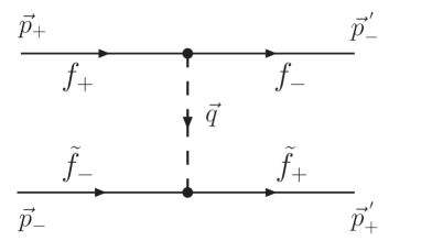
Figure 5: Tree-level Feynman diagram for one-magnon exchange between two holes.

Evaluating these Feynman diagrams, in momentum space one arrives at the following potentials for various combinations of flavors $f,\tilde{f}\in\{\alpha,\beta\}$ and couplings $F,\tilde{F}\in\{\Lambda,K\}$

$$\langle\vec{p}_{+}\ \!\!\!\!^{\prime}\,\vec{p}_{-}\ \!\!\!\!^{\prime}|V^{f\tilde{f}}_{F\tilde{F}}|\vec{p}_{+}\vec{p}_{-}\rangle=V^{f\tilde{f}}_{F\tilde{F}}(\vec{q}\,)\ \delta(\vec{p}_{+}+\vec{p}_{-}-\vec{p}_{+}\ \!\!\!\!^{\prime}-\vec{p}_{-}\ \!\!\!\!^{\prime}),\qquad F,\tilde{F}\in\left\{\Lambda,K\right\},$$ (5.3)

with

$$V^{ff}_{\Lambda\Lambda}(q) =-\frac{\Lambda^{2}}{2\rho_{s}},\qquad V^{ff^{\prime}}_{\Lambda\Lambda}(q)=\frac{\Lambda^{2}}{2\rho_{s}q^{2}}\big{(}iq_{1}-\sigma_{f}q_{2}\big{)}^{2},$$

$$V^{ff}_{KK}(q) =-\frac{K^{2}}{2\rho_{s}}\big{[}2(p_{+1}-i\sigma_{f}p_{+2})-q_{1}+i\sigma_{f}q_{2}\big{]}\big{[}2(p_{-1}+i\sigma_{f}p_{-2})+q_{1}+i\sigma_{f}q_{2}\big{]},$$

$$V^{ff^{\prime}}_{KK}(q) =-\frac{K^{2}}{2\rho_{s}q^{2}}\big{(}q_{1}-i\sigma_{f}q_{2}\big{)}^{2}\big{[}2(p_{+1}-i\sigma_{f}p_{+2})-q_{1}+i\sigma_{f}q_{2}\big{]}$$

$$\times\big{[}2(p_{-1}-i\sigma_{f}p_{-2})+q_{1}-i\sigma_{f}q_{2}\big{]},$$

$$V^{ff}_{\Lambda K}(q) =-\frac{i\Lambda K}{2\rho_{s}q^{2}}\big{(}q_{1}+i\sigma_{f}q_{2}\big{)}^{2}\big{[}2(p_{-1}+i\sigma_{f}p_{-2})+q_{1}+i\sigma_{f}q_{2}\big{]},$$

$$V^{ff^{\prime}}_{\Lambda K}(q) =-\frac{i\Lambda K}{2\rho_{s}}\big{[}2(p_{-1}-i\sigma_{f}p_{-2})+q_{1}-i\sigma_{f}q_{2}\big{]},$$

$$V^{ff}_{K\Lambda}(q) =\frac{iK\Lambda}{2\rho_{s}q^{2}}\big{(}q_{1}-i\sigma_{f}q_{2}\big{)}^{2}\big{[}2(p_{+1}-i\sigma_{f}p_{+2})-q_{1}+i\sigma_{f}q_{2}\big{]},$$

$$V^{ff^{\prime}}_{K\Lambda}(q) =\frac{iK\Lambda}{2\rho_{s}}\big{[}2(p_{+1}-i\sigma_{f}p_{+2})-q_{1}+i\sigma_{f}q_{2}\big{]}.$$ (5.4)

We noted earlier that the leading contribution to the low-energy physics comes from the $\Lambda$-vertex. From here on, we therefore concentrate on the potential with two $\Lambda$ vertices only. In coordinate space the $\Lambda\Lambda$-potentials are given by

$$\langle\vec{r}_{+}\ \!\!\!\!^{\prime}\vec{r}_{-}\ \!\!\!\!^{\prime}|V^{f\tilde{f}}_{\Lambda\Lambda}|\vec{r}_{+}\vec{r}_{-}\rangle=V^{f\tilde{f}}_{\Lambda\Lambda}(\vec{r}\,)\ \delta(\vec{r}_{+}-\vec{r}_{-}\ \!\!\!\!^{\prime})\ \delta(\vec{r}_{-}-\vec{r}_{+}\ \!\!\!\!^{\prime}),$$ (5.5)

with

$$V^{ff}_{\Lambda\Lambda}(\vec{r}\,)=-\frac{\Lambda^{2}}{2\rho_{s}}\delta^{(2)}(\vec{r}\,),\qquad V^{ff^{\prime}}_{\Lambda\Lambda}(\vec{r}\,)=\frac{\Lambda^{2}}{2\pi\rho_{s}\vec{r}^{\,2}}\exp(2i\sigma_{f}\varphi).$$ (5.6)

Here $\vec{r}=\vec{r}_{+}-\vec{r}_{-}$ denotes the distance vector between the two holes and $\varphi$ is the angle between $\vec{r}$ and the $x_{1}$-axis. The $\delta$-functions in Eq.(5.5) ensure that the holes do not change their position during the magnon exchange. It should be noted that the one-magnon exchange potentials are instantaneous although magnons travel with the finite speed c. Retardation effects occur only at higher orders.

Interestingly, in the $\Lambda\Lambda$ channel, one-magnon exchange over long distances between two holes can only happen for holes of opposite flavor. For two holes of the same flavor, one-magnon exchange acts as a contact interaction. In the next section we will concentrate on the long-range physics of weakly bound states of holes and therefore we will only consider the binding of holes of different flavor.

6 Two-Hole Bound States

We now investigate the Schrödinger equation for the relative motion of two holes with flavors $\alpha$ and $\beta$. In the following, we will treat short distance interactions by imposing a hard-core boundary condition on the pair’s wave function. Due to the accidental Galilean boost invariance, without loss of generality, we can consider the hole pair in its rest frame. The total kinetic energy of the two holes is given by

$$T=\sum_{f=\alpha,\beta}T^{f}=\sum_{f=\alpha,\beta}\frac{p_{i}^{2}}{2M^{\prime}}=\frac{p_{i}^{2}}{M^{\prime}}.$$ (6.1)

We introduce the two probability amplitudes $\Psi_{1}(\vec{r}\,)$ and $\Psi_{2}(\vec{r}\,)$ which represent the two flavor-spin combinations $\alpha_{+}\beta_{-}$ and $\alpha_{-}\beta_{+}$, respectively, where we choose the distance vector $\vec{r}$ to point from the $\beta$ to the $\alpha$ hole. Since the holes undergo a spin flip during the magnon exchange, the two probability amplitudes are coupled through the magnon exchange potentials and the Schrödinger equation describing the relative motion of the hole pair is a two-component equation. Using the explicit form of the potentials, the relevant Schrödinger equation for two holes reads

$$\left(\begin{array}[]{cc}-\frac{1}{M^{\prime}}\Delta&\gamma\frac{1}{\vec{r}^{\,2}}\exp(-2i\varphi)\\[0.86108pt] \gamma\frac{1}{\vec{r}^{\,2}}\exp(2i\varphi)&-\frac{1}{M^{\prime}}\Delta\end{array}\right)\left(\begin{array}[]{c}\Psi_{1}(\vec{r}\,)\\ \Psi_{2}(\vec{r}\,)\end{array}\right)=E\left(\begin{array}[]{c}\Psi_{1}(\vec{r}\,)\\ \Psi_{2}(\vec{r}\,)\end{array}\right),$$ (6.2)

with

$$\gamma=\frac{\Lambda^{2}}{2\pi\rho_{s}}.$$ (6.3)

Making the separation ansatz

$$\Psi_{1}(r,\varphi)=R_{1}(r)\exp(im_{1}\varphi),\qquad\Psi_{2}(r,\varphi)=R_{2}(r)\exp(im_{2}\varphi),$$ (6.4)

with $r=\left|\vec{r}\,\right|$, and using the Laplace operator in polar coordinates one arrives at the coupled equations

$$-\left(\frac{d^{2}}{dr^{2}}+\frac{1}{r}\frac{d}{dr}-\frac{1}{r^{2}}m_{1}^{2}\right)R_{1}(r)+\gamma M^{\prime}\frac{R_{2}(r)}{r^{2}}\exp\big{(}-i\varphi(2+m_{1}-m_{2})\big{)} =M^{\prime}ER_{1}(r),$$

$$-\left(\frac{d^{2}}{dr^{2}}+\frac{1}{r}\frac{d}{dr}-\frac{1}{r^{2}}m_{2}^{2}\right)R_{2}(r)+\gamma M^{\prime}\frac{R_{1}(r)}{r^{2}}\exp\big{(}i\varphi(2+m_{1}-m_{2})\big{)} =M^{\prime}ER_{2}(r).$$ (6.5)

The radial and angular part can be separated provided that the condition $m_{2}-m_{1}=2$ is satisfied. Introducing the parameter $m$, which is implicitly defined by

$$m_{1}=m-1,\qquad m_{2}=m+1,$$ (6.6)

the radial equations are then given by

$$-\left(\frac{d^{2}}{dr^{2}}+\frac{1}{r}\frac{d}{dr}-\frac{1}{r^{2}}(m-1)^{2}\right)R_{1}(r)+\gamma M^{\prime}\frac{R_{2}(r)}{r^{2}} =M^{\prime}ER_{1}(r),$$

$$-\left(\frac{d^{2}}{dr^{2}}+\frac{1}{r}\frac{d}{dr}-\frac{1}{r^{2}}(m+1)^{2}\right)R_{2}(r)+\gamma M^{\prime}\frac{R_{1}(r)}{r^{2}} =M^{\prime}ER_{2}(r).$$ (6.7)

While the other cases would have to be investigated numerically, for $m=0$ the two radial equations decouple and can be solved analytically. In particular, by taking appropriate linear combinations, for $m=0$ the two equations can be cast into the form

$$\left[-\left(\frac{d^{2}}{dr^{2}}+\frac{1}{r}\frac{d}{dr}\right)+(1+\gamma M^{\prime})\frac{1}{r^{2}}\right]\big{(}R_{1}(r)+R_{2}(r)\big{)} =M^{\prime}E\big{(}R_{1}(r)+R_{2}(r)\big{)},$$

$$\left[-\left(\frac{d^{2}}{dr^{2}}+\frac{1}{r}\frac{d}{dr}\right)+(1-\gamma M^{\prime})\frac{1}{r^{2}}\right]\big{(}R_{1}(r)-R_{2}(r)\big{)} =M^{\prime}E\big{(}R_{1}(r)-R_{2}(r)\big{)}.$$ (6.8)

Because the two equations are different, but contain the same energy $E$, one of the equations has a vanishing solution. In the first equation the potential always has a positive sign and is thus repulsive. In the second equation, on the other hand, the potential has a negative sign and is therefore attractive when the low-energy constants obey the relation

$$1-\gamma M^{\prime}=1-\frac{M^{\prime}\Lambda^{2}}{2\pi\rho_{s}}\leq 0.$$ (6.9)

Thus, magnon-mediated forces can lead to bound states only if the low-energy constant $\Lambda$ is larger than the critical value

$$\Lambda_{c}=\sqrt{\frac{2\pi\rho_{s}}{M^{\prime}}}.$$ (6.10)

Interestingly, the same critical value arises in the investigation of spiral phases in a lightly doped antiferromagnet on the honeycomb lattice [23]. There it marks the point where spiral phases become energetically favorable compared to the homogeneous phase. Here we are interested in the solution of the above system where the first equation has a zero solution and the second a non-zero one, i.e. $R_{1}(r)+R_{2}(r)=0$. Identifying $R(r)=R_{1}(r)-R_{2}(r)$, the second equation takes the form

$$\left[-\left(\frac{d^{2}}{dr^{2}}+\frac{1}{r}\frac{d}{dr}\right)+(1-\gamma M^{\prime})\frac{1}{r^{2}}\right]R(r)=-M^{\prime}|E|R(r),$$ (6.11)

where we have set $E=-|E|$. The same equation occurred in the square lattice case [19, 20] and can be solved along the same lines. As it stands, the equation is ill-defined because the $1/r^{2}$ potential is too singular at the origin. However, we have not yet included the contact interaction proportional to the 4-fermion coupling $G_{3}$. Here, in order to keep the calculation analytically feasible, we model the short-range repulsion by a hard core radius $r_{0}$, i.e. we require $R(r_{0})=0$ for $r\leq r_{0}$. Eq.(6.11) is solved by a modified Bessel function

$$R(r)=AK_{\nu}\big{(}\sqrt{M^{\prime}|E|}r\big{)},\qquad\nu=i\sqrt{\gamma M^{\prime}-1},$$ (6.12)

with $A$ being a normalization constant. Demanding that the wave function vanishes at the hard core radius gives a quantization condition for the bound state energy. The quantum number $n$ then labels the $n$-th excited state. For large $n$, the binding energy is given by

$$E_{n}\sim-\frac{1}{M^{\prime}r_{0}^{2}}\exp\left(\frac{-2\pi n}{\sqrt{\gamma M^{\prime}-1}}\right).$$ (6.13)

Like every quantity calculated within the framework of the effective theory, the binding energy depends on the values of the low-energy constants. The binding is exponentially small in $n$ and there are infinitely many bound states. While the highly excited states have exponentially small energy, for sufficiently small $r_{0}$ the ground state could have a small size and be strongly bound. However, as already mentioned, for short-distance physics the effective theory should not be trusted quantitatively. If the holes were really tightly bound, one could construct an effective theory which incorporates them explicitly as relevant low-energy degrees of freedom. As long as the binding energy is small compared to the relevant high-energy scales, our result is valid and receives only small corrections from higher-order effects such as two-magnon exchange.

Finally, let us discuss the angular part of the wave equation. The ansatz (6.4) leads to the following solution for the ground state wave function

$$\Psi(r,\varphi)=\left(\begin{array}[]{c}\Psi_{1}(\vec{r}\,)\\ \Psi_{2}(\vec{r}\,)\end{array}\right)=R(r)\,\left(\begin{array}[]{c}\exp(-i\varphi)\\ -\exp(i\varphi)\end{array}\right).$$ (6.14)

Applying the 60 degrees rotation $O$ and using the transformation rules of Eq.(4.1) one obtains

$${}^{O}\Psi(r,\varphi)=-\,\Psi(r,\varphi).$$ (6.15)

Interestingly, the wave function for the ground state of two holes of flavors $\alpha$ and $\beta$ thus exhibits $f$-wave symmetry. The corresponding probability distribution depicted in Figure 6, on the other hand, seems to show $s$-wave symmetry. However, the relevant phase information is not visible in this picture, because only the probability density is shown.

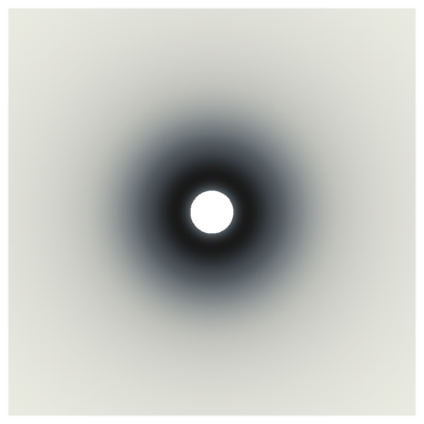
Figure 6: Probability distribution for the ground state of two holes of flavors $\alpha$ and $\beta$.

Interestingly, for two-hole bound states on the square lattice, the wave function for the the ground state of two holes of flavors $\alpha$ and $\beta$ shows $p$-wave symmetry, while the corresponding probability distribution (which again does not contain the relevant phase information) resembles $d_{x^{2}-y^{2}}$ symmetry [19]. Remarkably, the ground state wave function (6.14) of a bound hole pair on the honeycomb lattice remains invariant under the reflection symmetry $R$, the shift symmetries $D_{i}$, as well as under the accidental continuous rotation symmetry $O(\gamma)$.

We would like to emphasize that the $f$-wave character of the two-hole bound state on the honeycomb lattice is an immediate consequence of the systematic effective field theory analysis. It seems that the issue of the true symmetry of the pairing state, realized in the dehydrated version of Na₂CoO${}_{2}\times y$H₂O is still controversial [30]. Still, it is quite interesting to note that a careful analysis of the available experimental data for this compound suggests that the pairing symmetry indeed is $f$-wave [31].

7 Conclusions

In complete analogy to our earlier investigations on the square lattice, we have constructed a systematic low-energy effective field theory of magnons and doped holes in an antiferromagnet on the honeycomb lattice. Due to the different lattice geometry, there are important symmetry differences which have an impact on the allowed terms that enter the effective Lagrangian. Interestingly, in contrast to the square lattice case, on the honeycomb lattice an accidental continuous spatial rotation invariance arises for the leading terms of the low-energy effective Lagrangian.

As an important result, we have identified the leading magnon-hole vertex which results from a term with a single uncontracted spatial derivative. This term, which is analogous to the Shraiman-Siggia term on the square lattice, yields a rather strong magnon-hole coupling since it appears at a low order in the systematic low-energy expansion. As we have investigated earlier, at non-zero hole doping, when $\Lambda$ is sufficiently strong, this term gives rise to spiral phases in the staggered magnetization [23].

In the present work, we have studied the effect of the magnon-hole vertex on two-hole bound states. Again in contrast to the square lattice case, it turned out that the magnon-hole coupling constant $\Lambda$ must exceed a critical value in order to obtain two-hole bound states. Our analysis implies that the wave function for the ground state of two holes of flavors $\alpha$ and $\beta$ exhibits $f$-wave symmetry (while the corresponding probability distribution seems to suggest $s$-wave symmetry). This is quite different from the square lattice case, where the wave function for the ground state of two holes of flavors $\alpha$ and $\beta$ exhibits $p$-wave symmetry (while the corresponding probability distribution resembles $d_{x^{2}-y^{2}}$ symmetry).

We like to stress again that the effective theory provides a theoretical framework in which the low-energy dynamics of lightly hole-doped antiferromagnets can be investigated in a systematic manner. Once the low-energy parameters have been adjusted appropriately by comparison with either experimental data or numerical simulations, the resulting physics is completely equivalent to the one of the Hubbard or $t$-$J$ model.

References

- [1] Z. Y. Meng, T. C. Lang, S. Wessel, F. F. Assaad, and A. Muramatsu, Nature 464, (2010) 847.
- [2] S. Chakravarty, B. I. Halperin, and D. R. Nelson, Phys. Rev. B39 (1989) 2344.
- [3] H. Neuberger and T. Ziman, Phys. Rev. B39 (1989) 2608.
- [4] D. S. Fisher, Phys. Rev. B39 (1989) 11783.
- [5] P. Hasenfratz and H. Leutwyler, Nucl. Phys. B343 (1990) 241.
- [6] P. Hasenfratz and F. Niedermayer, Phys. Lett. B268 (1991) 231.
- [7] P. Hasenfratz and F. Niedermayer, Z. Phys. B92 (1993) 91.
- [8] A. Chubukov, T. Senthil, and S. Sachdev, Phys. Rev. Lett. 72 (1994) 2089; Nucl. Phys. B426 (1994) 601.
- [9] B. I. Shraiman and E. D. Siggia, Phys. Rev. Lett. 60 (1988) 740; Phys. Rev. Lett. 61 (1988) 467; Phys. Rev. Lett. 62 (1989) 1564; Phys. Rev. B46 (1992) 8305.
- [10] M. Y. Kuchiev and O. P. Sushkov, Physica C218 (1993) 197.
- [11] O. P. Sushkov and V. N. Kotov, Phys. Rev. B70 (2004) 024503.
- [12] V. N. Kotov and O. P. Sushkov, Phys. Rev. B70 (2004) 195105.
- [13] H. Georgi, Weak Interactions and Modern Particle Theory, Benjamin-Cummings Publishing Company, 1984.
- [14] J. Gasser, M. E. Sainio, and A. Svarc, Nucl. Phys. B307 (1988) 779.
- [15] E. Jenkins and A. Manohar, Phys. Lett. B255 (1991) 558.
- [16] V. Bernard, N. Kaiser, J. Kambor, and U.-G. Meissner, Nucl. Phys. B388 (1992) 315.
- [17] T. Becher and H. Leutwyler, Eur. Phys. J. C9 (1999) 643.
- [18] F. Kämpfer, M. Moser, and U.-J. Wiese, Nucl. Phys. B729 (2005) 317.
- [19] C. Brügger, F. Kämpfer, M. Moser, M. Pepe, and U.-J. Wiese, Phys. Rev. B74 (2006) 224432.
- [20] C. Brügger, F. Kämpfer, M. Pepe, and U.-J. Wiese, Eur. Phys. J. B53 (2006) 433.
- [21] C. Brügger, C. P. Hofmann, F. Kämpfer, M. Pepe, and U.-J. Wiese, Phys. Rev. B75 (2007) 014421.
- [22] C. Brügger, C. P. Hofmann, F. Kämpfer, M. Moser, M. Pepe, and U.-J. Wiese, Phys. Rev. B75 (2007) 214405.
- [23] F.-J. Jiang, F. Kämpfer, C. P. Hofmann, and U.-J. Wiese, Eur. Phys. J. B69 (2009) 473.
- [24] S. Zhang, Phys. Rev. Lett. 65 (1990) 120.
- [25] C. N. Yang and S. Zhang, Mod. Phys. Lett. B4 (1990) 759.
- [26] F.-J. Jiang, F. Kämpfer, M. Nyfeler, and U.-J. Wiese, Phys. Rev. B78 (2008) 214406.
- [27] U.-J. Wiese and H. P. Ying, Z. Phys. B93 (1994) 147.
- [28] B. B. Beard and U.-J. Wiese, Phys. Rev. Lett 77 (1996) 5130.
- [29] U. Gerber, C. P. Hofmann, F.-J. Jiang, M. Nyfeler, and U.-J. Wiese, J. Stat. Mech. (2009) P03021.
- [30] N. B. Ivanova, S. G. Ovchinnikov, M. M. Korshunov, I. M. Eremin, and N. V. Kazak, Phys. Usp. 52 (2009) 789.
- [31] I. I. Mazin and M. D. Johannes, Nature Physics 1 (2005) 91.