The Bound State S-matrix of the Deformed Hubbard Chain

Abstract

In this work we use the $q$-oscillator formalism to construct the atypical (short) supersymmetric representations of the centrally extended $\mathcal{U}_{q}(\mathfrak{su}(2|2))$ algebra. We then determine the S-matrix describing the scattering of arbitrary bound states. The crucial ingredient in this derivation is the affine extension of the aforementioned algebra.

AEI-2011-062

1 Introduction

Integrable systems constitute a special class of models in mathematics and physics. Their properties allow them to be solved exactly and thus they form a very useful playground for studying various systems. One common feature shared by these models is that they are closely related to some underlying algebraic structures. Hence most of the quantum integrable systems exhibit a large and powerful symmetry algebra, for example of Yangian or quantum affine type. A particularly interesting example is the Hubbard model.

The Hubbard model, which was named after John Hubbard, is the simplest model of interacting particles on a lattice. It has only two terms in the Hamiltonian: the hopping term (kinetic energy) and the Coulomb potential Hubbard . The model describes an ensemble of particles in a periodic potential at sufficiently low temperatures such that all the particles may be considered to be in the lowest Bloch band. Moreover, any long-range interactions between the particles are considered to be weak enough and are consequently ignored. It is based on the tight-binding approximation of superconducting systems and the motion of electrons between the atoms of a crystalline solid. Despite its apparent simplicity, there are different applications and generalizations describing a plethora of interesting phenomena. In the case when interactions between particles on different sites of the lattice can not be neglected and are taken into account, the model is often referred to as the Extended Hubbard model. The particles can either be fermions, as in Hubbard’s original work, or bosons, and the model is then referred as either the Bose-Hubbard model or the boson Hubbard model. The latter can be used to study systems such as bosonic atoms on an optical lattice (for a decent overview of various generalizations see reprint volumes Hub1 ; Hub2 ; Hub3 and also a more recent book Hub4 ).

A very specific class of models that share features with the one-dimensional Hubbard model and the supersymmetric t-J model tJ is the so-called Alcaraz and Bariev model AB . It contains an extra spin-spin interaction term in the Hamiltonian and it shows some characteristics of superconductivity. This model can be viewed as a quantum deformation of the Hubbard model in much the same way as the Heisenberg XXZ model is a quantum deformation of the XXX model. This model has a specific R-matrix which can not be written as a function of the difference of two associated spectral parameters. This paradigm is related to the very interesting but at the same time complicated algebraic properties of the model.

In recent years there has been renewed interest in integrable models arising from the discovery of integrable structures in the context of the AdS/CFT correspondence. For a recent review see AdSReview and references therein. The worldsheet S-matrix encountered there is one of the central objects of research and it turns out to have a lot in common with the specific cases of the Hubbard model considered in BAnalytic ; BK . Interestingly, the S-matrix of such a Hubbard model is obtained as a special limit of this worldsheet S-matrix MartinsMelo .

The exact integrability of the one-dimensional Hubbard model was established by B. Shastry Shastry . It was also shown that the model exhibits $\mathcal{Y}(\mathfrak{su}(2))\oplus\mathcal{Y}(\mathfrak{su}(2))$ Yangian symmetry UK . However this symmetry is insufficient to constrain Shastry’s S-matrix completely. Similarly, the worldsheet S-matrix for the ${\rm AdS}_{5}\times{\rm S}^{5}$ superstring also turns out to have Yangian symmetry BeisertYangian . However the Yangian in this model is based on a larger Lie algebra, the centrally extended $\mathfrak{su}(2|2)$ Lie superalgebra. This underlying Lie superalgebra turns out to be powerful enough to constrain the S-matrix BeisertFundamental ; AFZ ; BJ (up to an overall phase, the so-called ‘dressing factor’ Janik ; AFS ; BES ) in the case where at least one of the representations is fundamental. However, Yangian symmetry (or equivalently the Yang-Baxter equation) is required in order to find the S-matrix describing the scattering of states that live in higher representations AFBound ; MdLrmat . This specifically concerns the bound states in the system which transform in supersymmetric short representations Bsu22 ; Dorey ; CDO ; CDO2 . The bound state scattering matrix can be explicitly constructed with the help of the underlying Yangian symmetry ALT .

Nevertheless, there are still some problems concerning this infinite dimensional Yangian algebra due to some of its unusual features. The centrally extended $\mathfrak{su}(2|2)$ Lie superalgebra has a degenerate Cartan matrix which prohibits the direct application of most of techniques related to the theory of Yangians. For the case at hand this has been partially circumvented in several ways: by enlarging the algebra by an $\mathfrak{sl}(2)$ automorphisms BeisertYangian , by considering the $\alpha\to 0$ limits of the exceptional Lie superalgebra $\mathfrak{d}(2,1;\alpha)$ MM or building Drinfeld’s second realization ST . However this still proves to be an obstacle when, for example, one tries to construct the universal R-matrix ALTlong ; ALTblocks . This object encodes all the scattering data in the theory in a purely algebraic form. Another issue that is not completely understood is the appearance of the so-called secret symmetry MMT . This is an additional symmetry of the S-matrix that does not have a corresponding Lie algebraic generator in the extended $\mathfrak{su}(2|2)$ and could be interpreted as a $\mathfrak{u}(1)$ outer automorphism of $\mathfrak{su}(2|2)$. Resolving these issues could shed some light on the underlying algebraic structures and put the methods used to solve the model on a more firm footing.

A possible route for attacking these issues was put forward in BK , where the quantum deformation $\mathcal{Q}$ of the extended $\mathfrak{su}(2|2)$ algebra was studied. This $q$-deformed algebra has a number of interesting features such as a rather symmetric realization of the different central elements. Excitingly, just as in the non-deformed case, there is a link to Hubbard models, more specifically it describes spectrum of deformed supersymmetric one-dimensional Hubbard models DFFR ; BK . The undeformed Hubbard model is revealed by taking a specific limit of deformed model Bcl . Moreover, by sending the quantum deformation parameter $q\to 1$, the S-matrix under the consideration reduces to the AdS/CFT worldsheet S-matrix. As such, this matrix encompasses both different varieties of Hubbard models as well as the AdS/CFT worldsheet S-matrix and seems to provide a unifying algebraic framework for describing this class of models.

The $q$-deformed S-matrix in the fundamental representation is constrained up to an overall phase by requiring invariance under $\mathcal{Q}$ itself. However, in the light that both the AdS/CFT and the Hubbard model S-matrices are actually invariant under an infinite dimensional symmetry algebra, it should not be surprising that such a structure is also present here. Indeed, the larger algebraic structure underlying this S-matrix is the quantum affine algebra $\widehat{\cal{Q}}$ BGM . This infinite dimensional algebra is obtained by adding an additional fermionic node to the Dynkin diagram of $\mathcal{Q}$. In the $q\to 1$ limit one can retrieve the Yangian generators of centrally extended $\mathfrak{su}(2|2)$ by considering the appropriate combinations of generators of $\widehat{\cal{Q}}$. This fuels the idea that $\widehat{\cal{Q}}$ plays a similar role as the Yangian in the undeformed case. More specifically, it is expected that the S-matrix in the higher representations is uniquely defined up to an overall phase by the underlying quantum affine algebra $\widehat{\cal{Q}}$. This indeed turns out to be the case as we will show in this work.

The class of representations we are considering in this work are the supersymmetric short representations. These representations are called short because the central elements are not independent; they satisfy the so-called shortening condition Bsu22 . In order to construct these representations, we employ the formalism of quantum oscillators. It is a quantum version of the well-known harmonic oscillator algebra and is defined as

$$[N,\mathsf{a}]=-\mathsf{a}, [N,\mathsf{a}^{\dagger}]=\mathsf{a}^{\dagger}, \mathsf{a}\,\mathsf{a}^{\dagger}-q\,\mathsf{a}^{\dagger}\mathsf{a}=q^{-N}.$$

The use of quantum oscillators in the context of quantum groups was investigated earlier in Macfarlane ; Biedenharn ; Hayashi . By employing Fock space type modules, $q$-oscillators naturally give rise to the representations of quantum groups. This approach was first formulated for the quantum deformed algebra $\mathcal{U}_{q}(\mathfrak{sl}(2))$ and later extended to simple Lie (super)algebras of a more general type, see e.g. Chaichian . Since then quantum oscillators have become an important part of the theory of quantum deformed algebras.

Apart from being an interesting mathematical playground for studying the quantum affine algebra $\widehat{\cal{Q}}$ and its S-matrix, there is also a more elaborate motivation for considering these representations and the corresponding S-matrix. Firstly, there might be some possible applications in the context of the deformed Hubbard model. Secondly, it turns out that bound state states transform exactly in these representations of $q$-oscillator algebra. It is important to study bound states for many reasons. For example, bound states usually play a crucial role in the thermodynamics of the model. In the case of the non-deformed model in AdS/CFT, the thermodynamic Bethe ansatz (TBA) formalism is key in describing the complete spectrum of the theory AFstring ; GKV ; BFT ; AFTBA . The bound state S-matrix then governs the large volume solutions of both the TBA equations and the Y-system. Thus this is one of the first steps towards the TBA and Y-system formalism for the $q$-deformed model. And, consequently, it might give some useful insights in these structures in the context of the AdS/CFT superstring. For example, there might be an interesting link to the recently constructed $q$-deformed Pohlmeyer reduced version of the superstrings in the ${\rm AdS}_{5}\times{\rm S}^{5}$ background HT ; HHM which seems to be closely related to the $q$-deformed model constructed in BK .

In this work we derive the matrix structure of the general bound state S-matrix by employing the methods used in the context of the AdS/CFT superstring ALT , but rather than using the Yangian symmetry we make use of the underlying quantum affine algebra $\widehat{\cal{Q}}$. Our approach is based on the identification of invariant subspaces in the scattering theory that are specified by their invariance properties under the Cartan elements of the algebra. Then we use the rest of the algebra generators to relate these subspaces to each other resulting in the explicit form of the corresponding S-matrix. Just as in ALT we find the S-matrix in a factorized form reminiscent of the Drinfeld twist Drinfeld .

The paper is organized as follows. In section 2 we discuss the quantum deformation $\mathcal{Q}$ of the extended $\mathcal{U}(\mathfrak{su}(2|2))$ algebra and its affine extension $\widehat{\cal{Q}}$. Then in section 3 we introduce the quantum oscillator formalism and construct the supersymmetric short representations of $\widehat{\cal{Q}}$. In section 4 we present the explicit derivation of the S-matrix for these representations. Subsequently, in section 5, we specify some explicit cases, we reproduce the fundamental R-matrix and also we give the precise form of the scattering matrix when one of the spaces forms a fundamental representation. We end with a brief discussion on the results and interesting directions for future research. The majority of the S-matrix coefficients and results of the intermediate steps of the performed calculations are spelled out in the appendices.

2 Quantum affine algebra of extended $\mathcal{U}_{q}(\mathfrak{su}(2|2))$

In this section we review the quantum deformation of the extended $\mathfrak{su}(2|2)$ algebra BK and its affine extension BGM .

2.1 Quantum deformation of extended $\mathfrak{su}(2|2)$

The quantum deformed extended $\mathfrak{su}(2|2)$ algebra $\mathcal{Q}$ was introduced in BK . This algebra is generated by the three sets of Chevalley-Serre generators $\{E_{j},K_{j},F_{j}\}$ ($j=1,2,3$) where $E_{j}$ and $F_{j}$ are raising and lowering generators respectively and $K_{j}=q^{H_{j}}$ are the Cartan generators. We will consider the case when $E_{2}$ and $F_{2}$ are fermionic generators and the rest are bosonic. This corresponds to the $\mathfrak{su}(2|2)$ Dynkin diagram in Figure 1.

Figure 1: Dynkin diagram for the $\mathfrak{su}(2|2)$ algebra.

In addition, this algebra has two central charges $U$ and $V=q^{C}$ and two parameters: the deformation parameter $q$ and the coupling constant $g$. There is also a third parameter $\alpha$, which describes the relative scaling of $E_{2}$ and $F_{2}$. Even though it is possible absorb this parameter into thes generators by a suitable redefinition, we will keep it unspecified.

Algebra.

The commutation relations which include the mixed Chevalley-Serre generators are ($j,k=1,2,3$)

$$K_{j}E_{k}=q^{+DA_{jk}}E_{k}K_{j},\qquad K_{j}F_{k}=q^{-DA_{jk}}F_{k}K_{j},\qquad[E_{j},F_{k}\}=D_{jj}\delta_{jk}\frac{K_{j}-K^{-1}_{j}}{q-q^{-1}},$$ (1)

where the associated Cartan matrix $A$ and normalization matrix $D$ are given by

$$DA=\left(\begin{array}[]{rrr}+2&-1&0\\ -1&0&+1\\ 0&+1&-2\\ \end{array}\right),\qquad D=\mathrm{diag}(+1,-1,-1)\;.$$ (5)

There are also the unmixed commutation relations, called the Serre relations ($j=1,3$),

$$[E_{1},E_{3}]=\{E_{2},E_{2}\}=\bigl{[}E_{j},[E_{j},E_{2}]\bigr{]}-(q-2+q^{-1})E_{j}E_{2}E_{j}=0,$$

$$[F_{1},F_{3}]=\{F_{2},F_{2}\}=\bigl{[}F_{j},[F_{j},F_{2}]\bigr{]}-(q-2+q^{-1})F_{j}F_{2}F_{j}=0.$$ (6)

In addition, this algebra satisfies the extended Serre relations that give rise to two central elements $U$ and $V$ as follows,

$$g\alpha(1-U^{2}V^{2}) =\bigl{\{}[E_{2},E_{1}],[E_{2},E_{3}]\bigr{\}}-(q-2+q^{-1})E_{2}E_{1}E_{3}E_{2},$$

$$g\alpha^{-1}(V^{-2}-U^{-2}) =\bigl{\{}[F_{2},F_{1}],[F_{2},F_{3}]\bigr{\}}-(q-2+q^{-1})F_{2}F_{1}F_{3}F_{2}.$$ (7)

The central element $V$ is also related to the Cartan generators through

$$V^{-2} =K_{1}K_{2}^{2}K_{3}\;.$$ (8)

The conventional $\mathcal{U}_{q}(\mathfrak{su}(2|2))$ algebra is obtained in the limit $g\to 0$.

Coalgebra.

The defining relations of $\mathcal{Q}$ are compatible with the following coalgebra structure. The coproduct of the group like elements $X\in\{U,V,K\}$ is ${\rm\Delta}(X)=X\otimes X$ and the coproducts of the Chevalley-Serre generators $E_{j}$ and $F_{j}$ ($j=1,3$) take the standard forms. However the coproducts of the fermionic generators $E_{2}$ and $F_{2}$ involve an additional braiding factor $U$, which is one of the central charges of the algebra alluded to in the previous paragraph,

$${\rm\Delta}(E_{j})=E_{j}\otimes 1+K^{-1}_{j}U^{+\delta_{j,2}}\otimes E_{j},\qquad{\rm\Delta}(F_{j})=F_{j}\otimes K_{j}+U^{-\delta_{j,2}}\otimes F_{j}.$$ (9)

The coalgebra can be extended to a Hopf algebra. We will give the relevant definitions of the antipode and counit later on.

2.2 Affine Extension

The infinite dimensional quantum affine algebra $\widehat{\cal{Q}}$ is the affine extension of ${\mathcal{Q}}$ introduced in BGM . The affine extension is obtained by adding an additional node into the Dynkin diagram as depicted in Figure 2.

Figure 2: Dynkin diagram for the affine $\widehat{\mathfrak{su}}(2|2)$ algebra.

The remarkable property of this diagram is that the additional fermionic node is a copy of the second node. Therefore, we introduce the affine Chevalley-Serre generators $\{E_{4},F_{4},K_{4}\}$ as copies of $\{E_{2},F_{2},K_{2}\}$ and assume that they satisfy the same commutation relations as are given in (1), (2.1) and (2.1) and also have the same coalgebra structure (9). Thus, we introduce an additional set of the parameters $g,\alpha$ and central charges $U,V$. We distinguish these two sets by adhering subscripts to them arising from the generators to which they are associated,

$$g\to g_{k},\qquad\alpha\to\alpha_{k},\qquad U\to U_{k},\qquad V\to V_{k},\qquad\text{with}\qquad k=2,4.$$ (10)

Next, we need to determine the commutation relations $\{E_{2},F_{4}\}$ and $\{E_{4},F_{2}\}$ in such way that they would be compatible with the coalgebra structure,

$${\rm\Delta}(\{E_{2},F_{4}\})=\{{\rm\Delta}(E_{2}),{\rm\Delta}(F_{4})\}\qquad\text{and}\qquad{\rm\Delta}(\{E_{4},F_{2}\})=\{{\rm\Delta}(E_{4}),{\rm\Delta}(F_{2})\}\;.$$ (11)

Algebra.

As a result, we obtain the quantum affine algebra $\widehat{\cal{Q}}$ BGM . The mixed commutation relations of it are given by ($i,j=1,3$)

$$K_{i}E_{j} =q^{+DA_{ij}}E_{j}K_{i}, K_{i}F_{j} =q^{-DA_{ij}}F_{j}K_{i},$$

$$\{E_{2},F_{4}\} =-\tilde{g}\tilde{\alpha}^{-1}(K_{4}-U_{2}U_{4}^{-1}K_{2}^{-1}), \{E_{4},F_{2}\} =\tilde{g}\tilde{\alpha}(K_{2}-U_{4}U_{2}^{-1}K_{4}^{-1}),$$

$$[E_{j},F_{j}\} =D_{jj}\frac{K_{j}-K_{j}^{-1}}{q-q^{-1}} [E_{i},F_{j}\} =0,\quad\text{for}~{}~{}i\neq j,\ i+j\neq 6\;.$$ (12)

with the two new constants $\tilde{g}$ and $\tilde{\alpha}$ and the associated supersymmetric Cartan matrix $A$ and normalization matrix $D$ given by

$$DA=\left(\begin{array}[]{rrrr}+2&-1&0&-1\\ -1&0&+1&0\\ 0&+1&-2&+1\\ -1&0&+1&0\end{array}\right),\qquad D=\mathrm{diag}(1,-1,-1,-1).$$ (17)

These are supplemented by the following Serre relations ($j=1,3$ and $k=2,4$)

$$[E_{1},E_{3}]=E_{2}E_{2}=E_{4}E_{4}=\{E_{2},E_{4}\}=0\;,$$

$$[F_{1},F_{3}]=F_{2}F_{2}=F_{4}F_{4}=\{F_{2},F_{4}\}=0\;,$$

$$[E_{j},[E_{j},E_{k}]]-(q-2+q^{-1})E_{j}E_{k}E_{j}=0\;,$$

$$[F_{j},[F_{j},F_{k}]]-(q-2+q^{-1})F_{j}F_{k}F_{j}=0\;.$$ (18)

The central charges are related to the quartic Serre relations as ($k=2,4$)

$$g_{k}\alpha_{k}(1-U_{k}^{2}V_{k}^{2}) =\bigl{\{}[E_{k},E_{1}],[E_{k},E_{3}]\bigr{\}}-(q-2+q^{-1})E_{k}E_{1}E_{3}E_{k}\;,$$

$$g_{k}\alpha_{k}^{-1}(V_{k}^{-2}-U_{k}^{-2}) =\bigl{\{}[F_{k},F_{1}],[F_{k},F_{3}]\bigr{\}}-(q-2+q^{-1})F_{k}F_{1}F_{3}F_{k}\;.$$ (19)

and the central charges $V_{k}$ are related with Cartan charges through ($k=2,4$)

$$V^{-2}_{k} =K_{1}K_{k}^{2}K_{3}\;.$$ (20)

Coalgebra.

The group-like elements $X\in\{1,K_{j},U_{k},V_{k}\}$ ($j=1,2,3,4$ and $k=2,4$) have the coproduct ${\rm\Delta}$, the antipode ${\rm S}$ and the counit $\varepsilon$ defined in the usual way,

$$\Delta(X)=X\otimes X,\qquad S(X)=X^{-1},\qquad\varepsilon(X)=1,$$ (21)

while the coproducts of the Chevalley-Serre generators are deformed by the central elements $U_{k}$ as follows ($j=1,2,3,4$),

$$\Delta(E_{j}) =E_{j}\otimes 1+K_{j}^{-1}U_{2}^{+\delta_{j,2}}U_{4}^{+\delta_{j,4}}\otimes E_{j}, {\rm S}(E_{j}) =-U_{2}^{-\delta_{j,2}}U_{4}^{-\delta_{j,4}}K_{j}E_{j}, \varepsilon(E_{j}) =0,$$

$$\Delta(F_{j}) =F_{j}\otimes K_{j}+U_{2}^{-\delta_{j,2}}U_{4}^{-\delta_{j,4}}\otimes F_{j}, {\rm S}(F_{j}) =-U_{2}^{+\delta_{j,2}}U_{4}^{+\delta_{j,4}}F_{j}K_{j}^{-1}, \varepsilon(F_{j}) =0.$$ (22)

It is important to note that the above coproducts are compatible with all the defining relations, including the commutators $\{E_{2},F_{4}\}$ and $\{E_{4},F_{2}\}$ in (2.2). The opposite coproduct is defined as $\Delta^{\!op}=\mathcal{P}\,\Delta\,\mathcal{P}$ with $\mathcal{P}$ being the graded permutation operator.

Parameter constraints.

In general, the quantum affine algebra $\widehat{\cal{Q}}$ has seven parameters $g_{k},\alpha_{k},\tilde{\alpha},\tilde{g},q$ ($k=2,4$). A suitable choice of them which lead to an interesting fundamental representation was performed in BGM :

$$g_{2}=g_{4}=g,\qquad\alpha_{2}=\alpha_{4}\,\tilde{\alpha}^{-2}=\alpha,\qquad\tilde{g}^{2}=\frac{g^{2}}{1-g^{2}(q-q^{-1})^{2}}\,.$$ (23)

This choice of parameters is also compatible with the bound state representations. Thus in this paper we only consider the quantum affine algebra $\widehat{\cal{Q}}$, parametrized by four independent parameters $g,\alpha,\tilde{\alpha},q$ given in the relations above.

3 Quantum oscillators and representations

In this section we will provide all the necessary background for constructing the bound state S-matrix for the $q$-deformed Hubbard model. We will build the bound state representation by introducing $q$-oscillator formalism linking it to the aforementioned quantum affine algebra.

3.1 q-Oscillators

We first introduce the notion of $q$-oscillators and discuss how to obtain the representations of the quantum deformed algebras using $q$-oscillators. A concise overview of the $q$-oscillators and their relation to such representations may be found in ChaichianBook ; Petersen .

Definitions.

The $q$-oscillator ($q$-Heisenberg-Weyl algebra) $\mathcal{U}_{q}(\mathfrak{h}_{4})$ is the associative unital algebra consisting of the generators $\{\mathsf{a}^{\dagger},\mathsf{a},w,w^{-1}\}$ that satisfy the following relations,

$$w\,\mathsf{a}^{\dagger} =q\,\mathsf{a}^{\dagger}w, qw\,\mathsf{a}=\mathsf{a}\,w,$$ (24)

$$ww^{-1} =w^{-1}w=1, \mathsf{a}\,\mathsf{a}^{\dagger}-q\,\mathsf{a}^{\dagger}\mathsf{a}=w^{-1}.$$

From the defining relations one can see that the element $w^{-1}(\mathsf{a}^{\dagger}\mathsf{a}-\frac{w-w^{-1}}{q-q^{-1}})$ is central. As such, we will set it to zero in the remainder. Then one easily obtains

$$\mathsf{a}^{\dagger}\mathsf{a}=\frac{w-w^{-1}}{q-q^{-1}}, \mathsf{a}\,\mathsf{a}^{\dagger}=\frac{qw-q^{-1}w^{-1}}{q-q^{-1}}.$$ (25)

We will also need to consider the fermionic version of the $q$-oscillator. The above notion is extended to include fermionic operators by adjusting the defining relations in the following way (we keep the same notation for bosonic and fermionic $\mathsf{a},\,\mathsf{a}^{\dagger}$ for now)

$$w\,\mathsf{a}^{\dagger} =q\,\mathsf{a}^{\dagger}w, qw\,\mathsf{a}=\mathsf{a}\,w,$$ (26)

$$ww^{-1} =w^{-1}w=1, \mathsf{a}\,\mathsf{a}^{\dagger}+q\,\mathsf{a}^{\dagger}\mathsf{a}=w.$$

In this case, the central element is $w(\mathsf{a}^{\dagger}\mathsf{a}-\frac{w-w^{-1}}{q-q^{-1}})$. Again we set this element to zero, resulting in the following identities

$$\mathsf{a}^{\dagger}\mathsf{a}=\frac{w-w^{-1}}{q-q^{-1}}, \mathsf{a}\,\mathsf{a}^{\dagger}=\frac{qw^{-1}-q^{-1}w}{q-q^{-1}}.$$ (27)

Of course in the fermionic case the operators $\mathsf{a},\mathsf{a}^{\dagger}$ square to zero. Equation (27) implies that this only is consistent if $w^{2}=1,q^{2}$. Below we will identify $w\equiv q^{N}$, where $N=0,1$ is the number of fermions making it indeed compatible.

Fock space.

The $q$-oscillator algebra can be used to define representations of $\mathcal{U}_{q}(\mathfrak{sl}(2))$ in a very simple way. Let us first build the Fock representation of $\mathcal{U}_{q}(\mathfrak{h}_{4})$. For this purpose consider a vacuum state $|0\rangle$ such that

$$\mathsf{a}|0\rangle=0,$$ (28)

then the Fock vector space $\cal{F}$ generated by the states of the form

$$|n\rangle=(\mathsf{a}^{\dagger})^{n}|0\rangle\,,$$ (29)

is an irreducible module of $\mathcal{U}_{q}(\mathfrak{h}_{4})$. Let us first consider the bosonic $q$-oscillators. With the help of the defining relations (24) and (25) one finds that the action of the oscillator algebra generators on this module is

$$\mathsf{a}^{\dagger}|n\rangle=|n+1\rangle, \mathsf{a}|n\rangle=[n]_{q}|n-1\rangle, w|n\rangle=q^{n}|n\rangle.$$ (30)

This makes it natural to identify $w\equiv q^{N}$, where $N$ is understood as a number operator. Analogously, fermionic generators are found to act as

$$\mathsf{a}^{\dagger}|n\rangle=|n+1\rangle, \mathsf{a}|n\rangle=[2-n]_{q}|n-1\rangle, w|n\rangle=q^{n}|n\rangle.$$ (31)

However, due to the fermionic nature, $n$ can only take the values $0$ and $1$ and thus the identity $[2-n]_{q}=[n]_{q}$ holds.

Next consider two copies of bosonic $q$-oscillators $\mathsf{a}_{i},\mathsf{a}^{\dagger}_{i},w_{i}=q^{N_{i}}$ which mutually commute. Then the Fock space is naturally spanned by vectors of the form

$$|m,n\rangle=(\mathsf{a}^{\dagger}_{1})^{m}(\mathsf{a}^{\dagger}_{2})^{n}|0\rangle.$$ (32)

It is easy to see that under the identification

$$E=\mathsf{a}^{\dagger}_{2}\mathsf{a}_{1}, F=\mathsf{a}^{\dagger}_{1}\mathsf{a}_{2}, H=N_{2}-N_{1},$$ (33)

the Fock space forms an infinite dimensional $\mathcal{U}_{q}(\mathfrak{sl}(2))$-representation. Moreover, the subspace $\mathcal{F}_{M}=\mathrm{span}\{\,|m,M-m\rangle\;|\;m=0,\ldots,M\,\}$ is an irreducible $\mathcal{U}_{q}(\mathfrak{sl}(2))$-representation of dimension $M+1$. This can be straightforwardly generalized to $\mathfrak{sl}(n)$ and more generally, by including fermionic oscillators, this space is extended to the representations of $\mathfrak{sl}(n|m)$ Chaichian .

Representations of centrally extended $\mathcal{U}_{q}(\mathfrak{su}(2|2))$.

We will now construct the bound state representation for centrally extended $\mathcal{U}_{q}(\mathfrak{su}(2|2))$ in the $q$-oscillator language. We need to consider two copies of $\mathfrak{sl}(2)$, a bosonic and a fermionic one. Thus we need four sets of $q$-oscillators $\mathsf{a}_{i},\mathsf{a}^{\dagger}_{i},w_{i}=q^{N_{i}}$, where the index $i=1,2$ denotes bosonic oscillators and $i=3,4$ – fermionic ones. Using these we write

$$E_{1}=\mathsf{a}^{\dagger}_{2}\mathsf{a}_{1}, F_{1}=\mathsf{a}^{\dagger}_{1}\mathsf{a}_{2}, H_{1}=N_{2}-N_{1},$$ (34)

$$E_{2}=a~{}\mathsf{a}^{\dagger}_{4}\mathsf{a}_{2}+b~{}\mathsf{a}^{\dagger}_{1}\mathsf{a}_{3} F_{2}=c~{}\mathsf{a}^{\dagger}_{3}\mathsf{a}_{1}+d~{}\mathsf{a}^{\dagger}_{2}\mathsf{a}_{4}, H_{2}=-C+\frac{N_{1}+N_{3}-N_{2}-N_{4}}{2},$$ (35)

$$E_{3}=\mathsf{a}^{\dagger}_{3}\mathsf{a}_{4}, F_{3}=\mathsf{a}^{\dagger}_{4}\mathsf{a}_{3}, H_{3}=N_{4}-N_{3},$$ (36)

where $C$ is central. It is then straightforward to check that this set of generators forms a representation of $\mathcal{U}_{q}(\mathfrak{su}(2|2))$ on the Fock space when restricting to the subspace of total particle number $M$ upon setting

$$ad=\frac{[C+{\textstyle\frac{M}{2}}]_{q}}{[M]_{q}}, bc=\frac{[C-{\textstyle\frac{M}{2}}]_{q}}{[M]_{q}}, ab=\frac{\mathfrak{P}}{[M]_{q}}, cd=\frac{\mathfrak{K}}{[M]_{q}}.$$ (37)

In the above $\mathfrak{K},\mathfrak{P}$ correspond to the right hand side of the Serre relations (2.2) following BK . As a consequence, the central charges satisfy the shortening condition

$$[C]_{q}^{2}-\mathfrak{PK}=\bigl{[}{\textstyle\frac{M}{2}}\bigr{]}_{q}^{2}.$$ (38)

Here the $q$-numbers are defined as

$$[k]_{q}=\frac{q^{k}-q^{-k}}{q-q^{-1}}.$$ (39)

This way of constructing representations of the centrally extended algebra reminds us of the procedure used in, e.g. ALTlong , where long representations were be obtained by twisting $\mathfrak{sl}(n|m)$ in a similar way.

In the $q\rightarrow 1$ limit the $q$-oscillators get reduced to regular oscillators and their representations coincide with the superspace formalism introduced in AFBound . The identification is as follows

$$\mathsf{a}_{1,2}\leftrightarrow\frac{\partial}{\partial w_{1,2}}, \mathsf{a}^{\dagger}_{1,2}\leftrightarrow w_{1,2}, \mathsf{a}_{3,4}\leftrightarrow\frac{\partial}{\partial\theta_{3,4}}, \mathsf{a}^{\dagger}_{3,4}\leftrightarrow\theta_{3,4}.$$ (40)

Parameterization and central elements.

Introducing $V=q^{C}$ and $U$ as in BGM , we rewrite (37) as

$$ad=\frac{q^{\frac{M}{2}}V-q^{-\frac{M}{2}}V^{-1}}{q^{M}-q^{-M}}, bc=\frac{q^{-\frac{M}{2}}V-q^{\frac{M}{2}}V^{-1}}{q^{M}-q^{-M}},$$

$$ab=\frac{g\alpha}{[M]_{q}}(1-U^{2}V^{2}), cd=\frac{g\alpha^{-1}}{[M]_{q}}(V^{-2}-U^{-2}).$$ (41)

which altogether leads to a constraint for $U$ and $V$,

$$\frac{g^{2}}{[M]_{q}^{2}}(V^{-2}-U^{-2})(1-U^{2}V^{2})=\frac{(V-q^{M}V^{-1})(V-q^{-M}V^{-1})}{(q^{M}-q^{-M})^{2}}\;.$$ (42)

This constraint agrees with the one in BGM by identifying $q\rightarrow q^{M},\;g\rightarrow g/[M]_{q}$. The explicit parametrization of the labels $a,b,c,d$ shall be given a bit further.

3.2 Affine extension

Next we want to consider the affine extension introduced in BGM . Here we will show that our representation allows an affine extension. Analogously to BGM we make the ansatz that the affine charges act as copies of $E_{2},F_{2},H_{2}$. In other words, we set

$$E_{4}=a_{4}~{}\mathsf{a}^{\dagger}_{4}\mathsf{a}_{2}+b_{4}~{}\mathsf{a}^{\dagger}_{1}\mathsf{a}_{3}, F_{4}=c_{4}~{}\mathsf{a}^{\dagger}_{3}\mathsf{a}_{1}+d_{4}~{}\mathsf{a}^{\dagger}_{2}\mathsf{a}_{4}, H_{4}=-C_{4}+\frac{N_{1}+N_{3}-N_{2}-N_{4}}{2}.$$ (43)

Checking all of the commutation relations is straightforward. Also, due to the defining relations (41), the equivalent expressions for the affine representation parameters are obtained

$$a_{4}d_{4}=\frac{q^{\frac{M}{2}}V_{4}-q^{-\frac{M}{2}}V_{4}^{-1}}{q^{M}-q^{-M}}, b_{4}c_{4}=\frac{q^{-\frac{M}{2}}V_{4}-q^{\frac{M}{2}}V_{4}^{-1}}{q^{M}-q^{-M}},$$

$$a_{4}b_{4}=\frac{g_{4}\alpha_{4}}{[M]_{q}}(1-U_{4}^{2}V_{4}^{2}), c_{4}d_{4}=\frac{g_{4}\alpha_{4}^{-1}}{[M]_{q}}(V_{4}^{-2}-U_{4}^{-2}).$$ (44)

However the commutators between the generators $E_{2}$ and $E_{4}$ and also between $F_{2}$ and $F_{4}$ induce relations between $a_{2},\,a_{4}$, etc. These are found to be

$$a_{2}d_{4} =\frac{\tilde{g}\tilde{\alpha}^{-1}}{[M]_{q}}(q^{\frac{M}{2}}U_{2}U_{4}^{-1}V_{2}-q^{-\frac{M}{2}}V_{4}^{-1}), b_{2}c_{4}=\frac{\tilde{g}\tilde{\alpha}^{-1}}{[M]_{q}}(q^{-\frac{M}{2}}U_{2}U_{4}^{-1}V_{2}-q^{\frac{M}{2}}V_{4}^{-1}),$$

$$c_{2}b_{4} =\frac{\tilde{g}\tilde{\alpha}}{[M]_{q}}(q^{\frac{M}{2}}V_{2}^{-1}-q^{-\frac{M}{2}}U_{2}^{-1}U_{4}V_{2}), d_{2}a_{4}=\frac{\tilde{g}\tilde{\alpha}}{[M]_{q}}(q^{-\frac{M}{2}}V_{2}^{-1}-q^{\frac{M}{2}}U_{2}^{-1}U_{4}V_{2}),$$ (45)

and agree with BGM upon sending $q\rightarrow q^{M},\,\tilde{g}\rightarrow\frac{\tilde{g}}{[M]_{q}}$, as in the non-affine case. The tilded $\tilde{g},\;\tilde{\alpha}$ are not independent but constrained parameters; thus there are 12 constraints for 12 parameters $\{a_{k},b_{k},c_{k},d_{k},U_{k},V_{k}\}$.

Hopf algebra and variables.

The Hopf algebra structure is just as previously discussed in Section 2. Here we will introduce Zhukowksy variables that will parameterize the representation labels $\{a_{k},b_{k},c_{k},d_{k}\}$ and central elements $U_{k},V_{k}$ for the bound-state representation. Following BGM we choose

$$g_{2}=g_{4}=g,\qquad\alpha_{2}=\alpha_{4}\,\tilde{\alpha}^{-2}=\alpha,\qquad\tilde{g}^{2}=\frac{g^{2}}{1-g^{2}(q-q^{-1})^{2}}.$$ (46)

Note that the powers of $q$ in the expressions above are $1$ and not $M$ because $g^{2}(q-q^{-1})^{2}$ is invariant under the bound state map $(g,\,q)\mapsto(g/[M]_{q},\,q^{M})$, thus these equations are identical to the ones for the fundamental representation.

Also, there is a relation between the central elements of the algebra,

$$U_{4}=\pm U_{2}^{-1},\qquad V_{4}=\pm V_{2}^{-1},$$ (47)

that are called the two-parameter family of the representation BGM . We shall be using the plus relation in our calculations.

The mass-shell constraint (multiplet shortening condition) obtained from the expressions (41) and (44) reads as

$$(a_{k}d_{k}-q^{M}b_{k}c_{k})(a_{k}d_{k}-q^{-M}b_{k}c_{k})=1,$$ (48)

and holds independently for $k=2,4$. In terms of the conventional $x^{\pm}$ parametrization it becomes

$$\frac{1}{q^{M}}\left(x^{+}+\frac{1}{x^{+}}\right)-q^{M}\left(x^{-}+\frac{1}{x^{-}}\right)=\left(q^{M}-\frac{1}{q^{M}}\right)\left(\xi+\frac{1}{\xi}\right),$$ (49)

where $\xi=-i\tilde{g}(q-q^{-1})$. One can further introduce a function $\zeta(x)$

$$\zeta(x)=-\frac{x+1/x+\xi+1/\xi}{\xi-1/\xi},$$ (50)

in terms of which (49) becomes $q^{-M}\zeta(x^{+})=q^{M}\zeta(x^{-})$. This parametrization leads to the following expressions of the labels $a_{k},b_{k},c_{k},d_{k}$ of a ‘canonical form’:

$$a_{k} =\sqrt{\frac{g}{[M]_{q}}}\gamma_{k}, b_{k}=\sqrt{\frac{g}{[M]_{q}}}\frac{\alpha_{k}}{\gamma_{k}}\frac{x^{-}_{k}-x^{+}_{k}}{x^{-}_{k}},$$

$$c_{k} =\sqrt{\frac{g}{[M]_{q}}}\frac{\gamma_{k}}{V_{k}\,\alpha_{k}}\frac{i\,q^{\frac{M}{2}}\tilde{g}}{g(x^{+}_{k}+\xi)}, d_{k}=\sqrt{\frac{g}{[M]_{q}}}\frac{V_{k}\,\tilde{g}\,q^{\frac{M}{2}}}{i\,g\,\gamma_{k}}\frac{x^{+}_{k}-x^{-}_{k}}{\xi x^{+}_{k}+1},$$ (51)

where the central charges are

$$U^{2}_{k}=\frac{1}{q^{M}}\frac{x^{+}_{k}+\xi}{x^{-}_{k}+\xi}=q^{M}\frac{x^{+}_{k}}{x^{-}_{k}}\frac{\xi x^{-}_{k}+1}{\xi x^{+}_{k}+1}, V^{2}_{k}=\frac{1}{q^{M}}\frac{\xi x^{+}_{k}+1}{\xi x^{-}_{k}+1}=q^{M}\frac{x^{+}_{k}}{x^{-}_{k}}\frac{x^{-}_{k}+\xi}{x^{+}_{k}+\xi},$$ (52)

and the relations between $x^{\pm}_{2},\;\gamma_{2}$ and $x^{\pm}_{4},\;\gamma_{4}$ are constrained by (45) to be

$$x_{2}^{\pm} =x^{\pm}, x_{4}^{\pm} =\frac{1}{x^{\pm}}, \gamma_{2} =\gamma, \gamma_{4} =\frac{i\tilde{\alpha}\gamma}{x^{+}}.$$ (53)

The relation between normalization coefficients $\alpha_{2}$ and $\alpha_{4}$ was given in (46). Finally, the convenient multiplicative evaluation parameter $z$ for the bound state representation is

$$z=q^{-M}\zeta(x^{+})=q^{M}\,\zeta(x^{-}).$$ (54)

3.3 Summary

For the convenience of the reader we want to summarize all expressions that will be used in the consequent calculations of the bound state S-matrix. We will slightly change the notation for parameters related to the fermionic nodes. We rename the representation parameters and the central elements of the algebra as

$$(a_{2},b_{2},c_{2},d_{2},U_{2},V_{2})\rightarrow(a,b,c,d,U,V),$$

$$(a_{4},b_{4},c_{4},d_{4},U_{4},V_{4})\rightarrow(\tilde{a},\tilde{b},\tilde{c},\tilde{d},{\widetilde{U}},{\widetilde{V}}),$$ (55)

in order to reserve the subscript position for denoting the momentum dependence, i.e. $a_{1}:=a(p_{1})$. in order to reserve the subscript position for discriminating states living in different tensor spaces. We will also give some relations that we found to be very useful.

Explicit representation.

The bound state representation is defined as

$$|m,n,k,l\rangle=(\mathsf{a}^{\dagger}_{3})^{m}(\mathsf{a}^{\dagger}_{4})^{n}(\mathsf{a}^{\dagger}_{1})^{k}(\mathsf{a}^{\dagger}_{2})^{l}\,|0\rangle.$$ (56)

The total number of excitations is $k+l+m+n=M$. The triple corresponding to the bosonic $\mathfrak{sl}(2)$ is given by

$$H_{1}|m,n,k,l\rangle=(l-k)|m,n,k,l\rangle,$$

$$E_{1}|m,n,k,l\rangle=[k]_{q}\,|m,n,k-1,l+1\rangle, F_{1}|m,n,k,l\rangle=[l]_{q}\,|m,n,k+1,l-1\rangle.$$ (57)

The fermionic part is

$$H_{3}|m,n,k,l\rangle=(n-m)|m,n,k,l\rangle,$$

$$E_{3}|m,n,k,l\rangle=|m+1,n-1,k,l\rangle, F_{3}|m,n,k,l\rangle=|m-1,n+1,k,l\rangle.$$ (58)

The action of the supercharges is given by

$$H_{2}|m,n,k,l\rangle= ~{}-\left\{C-\frac{k-l+m-n}{2}\right\}|m,n,k,l\rangle,$$

$$E_{2}|m,n,k,l\rangle= ~{}a~{}(-1)^{m}[l]_{q}\,|m,n+1,k,l-1\rangle+b~{}|m-1,n,k+1,l\rangle,$$

$$F_{2}|m,n,k,l\rangle= ~{}c~{}[k]_{q}\,|m+1,n,k-1,l\rangle+d~{}(-1)^{m}\,|m,n-1,k,l+1\rangle.$$ (59)

The parameters $a,b,c,d$ are related to the central charges via (37). The affine charges are defined exactly in the same way,

$$H_{4}|m,n,k,l\rangle= ~{}-\left\{\widetilde{C}-\frac{k-l+m-n}{2}\right\}|m,n,k,l\rangle,$$

$$E_{4}|m,n,k,l\rangle= ~{}\tilde{a}~{}(-1)^{m}[l]_{q}|m,n+1,k,l-1\rangle+\tilde{b}~{}|m-1,n,k+1,l\rangle,$$

$$F_{4}|m,n,k,l\rangle= ~{}\tilde{c}~{}[k]_{q}\,|m+1,n,k-1,l\rangle+\tilde{d}~{}(-1)^{m}\,|m,n-1,k,l+1\rangle.$$ (60)

The representation labels $a,b,c,d$ are given by

$$a =\sqrt{\frac{g}{[M]_{q}}}\gamma, b=\sqrt{\frac{g}{[M]_{q}}}\frac{\alpha}{\gamma}\frac{x^{-}-x^{+}}{x^{-}},$$

$$c =\sqrt{\frac{g}{[M]_{q}}}\frac{\gamma}{\alpha\,V}\frac{i\,q^{\frac{M}{2}}\tilde{g}}{g(x^{+}+\xi)}, d=\sqrt{\frac{g}{[M]_{q}}}\frac{\tilde{g}\,q^{\frac{M}{2}}V}{i\,g\,\gamma}\frac{x^{+}-x^{-}}{\xi x^{+}+1},$$ (61)

and the affine parameters $\tilde{a},\tilde{b},\tilde{c},\tilde{d}$ are acquired by replacing $V\to{\widetilde{V}}=V^{-1}$, $\gamma\to\frac{i\tilde{\alpha}\gamma}{x^{+}}$, $\alpha\to\,\alpha\,\tilde{\alpha}^{2}$ and $x^{\pm}\to\frac{1}{x^{\pm}}$; the corresponding central elements are given by $V=q^{C}$, ${\widetilde{V}}=q^{\widetilde{C}}$.

Useful relations.

The evaluation parameter $z$ may be expressed explicitly in terms of $x^{\pm}$ parametrization as

$$z\,(q-q^{-1})(\xi-\xi^{-1})=-\frac{1}{[M]_{q}}\Bigl{(}x^{+}-x^{-}+\frac{1}{x^{+}}-\frac{1}{x^{-}}\Bigr{)}.$$ (62)

Then using the identity

$$\xi-\xi^{-1}=\frac{\tilde{g}}{i(q-q^{-1})g^{2}},$$ (63)

one can further show that it is related to the representation labels (61) and their affine partners in a very nice way,

$$z=\frac{g}{\tilde{g}\,\alpha\,\tilde{\alpha}}(a\tilde{b}-b\tilde{a}),\qquad\frac{1}{z}=\frac{g\,\alpha\,\tilde{\alpha}}{\tilde{g}}(c\tilde{d}-d\tilde{c}),$$ (64)

while the consistency conditions (45) give

$$z=\frac{1-U^{2}V^{2}}{V^{2}-U^{2}}=\frac{1-{\widetilde{U}}^{2}{\widetilde{V}}^{2}}{{\widetilde{V}}^{2}-{\widetilde{U}}^{2}}\,.$$ (65)

Rational limit.

The rational limit is usually obtained by substituting $q=1+h$ and then finding the $h\to 0$ limit. Thus by defining the evaluation parameter (54) as $z=q^{-2u}$ we can expand it in series of $h$ as BGM

$$z=1-2hu+\mathcal{O}(h^{2}),\qquad\text{where}\qquad u=\frac{ig}{2}(x^{+}+x^{-})(1+1/x^{+}x^{-}).$$ (66)

It is noted that the $x^{\pm}$ parameters in (66) satisfies the leading order of the following relation which is stemming from the mass-shell constraint (49) in the $h\to 0$ limit,

$$x^{+}+\frac{1}{x^{+}}-x^{-}-\frac{1}{x^{-}}=\frac{iM}{g}+2hMu+\mathcal{O}(h^{2}).$$ (67)

In fact, this is consistent with the rational constraint for $x^{\pm}$ parameters ALT . Finally, it would be important to see how the representation parameters reduce in the rational limit. The representation labels (61) in the $q\to 1$ limit reduce to the usual (undeformed) labels $(a,b,c,d)$ of ALT . On the other hand, the affine parameters are related to the non-affine ones $(\tilde{a},\tilde{b},\tilde{c},\tilde{d})$ through BGM

$$M\widetilde{T}=\begin{pmatrix}z^{-1}&0\\ 0&1\end{pmatrix}T\begin{pmatrix}w^{-1}&0\\ 0&wz\end{pmatrix}\quad\text{with}\quad M=\begin{pmatrix}0&\alpha\tilde{\alpha}\\ -\alpha^{-1}\tilde{\alpha}^{-1}&0\end{pmatrix},\quad T=\begin{pmatrix}a&-b\\ -c&d\end{pmatrix}$$ (68)

where $z$ is the evaluation parameter given in (54), (65) and $w$ is defined by

$$w=\frac{\tilde{g}V}{gq^{1/2}}\frac{qU^{2}-1}{V^{2}U^{2}-1}=\frac{gq^{1/2}}{\tilde{g}V}\frac{U^{2}-V^{2}}{U^{2}-q}.$$ (69)

Since the central elements specialize to $(U,V)\to(\sqrt{\frac{x^{+}}{x^{-}}},1)$ in the limit $q\to 1$, it is easy to see that the matrix relation (68) reduces the following simple form,

$$M\widetilde{T}=T.$$ (70)

4 The S-matrix

We shall consider the bound state S-matrix which is an intertwining matrix of the tensor space furnished by the vectors

$$|m_{1},n_{1},k_{1},l_{1}\rangle\otimes|m_{2},n_{2},k_{2},l_{2}\rangle.$$ (71)

Here $0\leq m_{1},n_{1},m_{2},n_{2}\leq 1$ and $k_{1},l_{1},k_{2},l_{2}\geq 0$ denote the numbers of fermionic and bosonic excitations respectively with the bound state number $M_{i}$ being the total number of excitations $M_{i}=m_{i}+n_{i}+k_{i}+l_{i}$. Thus the S-matrix is the automorphism of the quantum deformed tensor space and is required to be invariant under the coproducts of the affine algebra $\widehat{\cal{Q}}$,

$${\mathbb{S}}\,\Delta(J)=\Delta^{op}(J)\,{\mathbb{S}},\qquad\text{for any}\qquad J\in\widehat{\cal{Q}}.$$ (72)

We normalize the S-matrix in such a way that the state $|0,0,0,M_{1}\rangle\otimes|0,0,0,M_{2}\rangle$ is invariant under the scattering. Therefore we will denote the state

$$|0\rangle=|0,0,0,M_{1}\rangle\otimes|0,0,0,M_{2}\rangle,$$ (73)

as the vacuum state.

The invariance under bosonic symmetries ${\Delta H}_{1}$ and ${\Delta H}_{3}$ requires the total number of fermions and the total number of fermions of one type

$$N_{f} =m_{1}+m_{2}+n_{1}+n_{2}+2l_{1}+2l_{2},$$

$$N_{f_{3}} =m_{1}+m_{2}+l_{1}+l_{2}.$$ (74)

to be conserved. This conservation divides the space (71) into five types of invariant subspaces of the S-matrix:

I   

$|0,1,k_{1},l_{1}\rangle\otimes|0,1,k_{2},l_{2}\rangle$,

Ib  

$|1,0,k_{1},l_{1}\rangle\otimes|1,0,k_{2},l_{2}\rangle$,

II  

$\{|0,0,k_{1},l_{1}\rangle\otimes|0,1,k_{2},l_{2}\rangle,|1,1,k_{1},l_{1}\rangle\otimes|0,1,k_{2},l_{2}\rangle,\\ \quad|0,1,k_{1},l_{1}\rangle\otimes|0,0,k_{2},l_{2}\rangle,|0,1,k_{1},l_{1}\rangle\otimes|1,1,k_{2},l_{2}\rangle\}$,

IIb

$\{|0,0,k_{1},l_{1}\rangle\otimes|1,0,k_{2},l_{2}\rangle,|1,1,k_{1},l_{1}\rangle\otimes|1,0,k_{2},l_{2}\rangle,\\ \quad|1,0,k_{1},l_{1}\rangle\otimes|0,0,k_{2},l_{2}\rangle,|1,0,k_{1},l_{1}\rangle\otimes|1,1,k_{2},l_{2}\rangle\}$,

III

$\{|0,0,k_{1},l_{1}\rangle\otimes|0,0,k_{2},l_{2}\rangle,|0,0,k_{1},l_{1}\rangle\otimes|1,1,k_{2},l_{2}\rangle,|1,1,k_{1},l_{1}\rangle\otimes|0,0,k_{2},l_{2}\rangle,\\ \quad|1,1,k_{1},l_{1}\rangle\otimes|1,1,k_{2},l_{2}\rangle,|0,1,k_{1},l_{1}\rangle\otimes|1,0,k_{2},l_{2}\rangle,|1,0,k_{1},l_{1}\rangle\otimes|0,1,k_{2},l_{2}\rangle\}$.

Subspaces I, Ib and II, IIb are isomorphic, hence we need to find the S-matrix for one of the isomorphic subspaces only. In the following we will consider the scattering in the subspaces I, II and III only.

The invariant subspaces differ by the numbers $N_{f,f_{3}}$. By considering the action of the algebra charges it is easy to see that the different subspaces are related to each other in the way shown in figure 3.

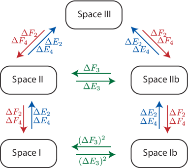
Figure 3: The invariant subspaces of the S-matrix and the algebraic relations between them.

Finally we want to give a remark on our choice of the basis. The $q$-oscillator basis we are considering is orthogonal, but not orthonormal,

$$\langle m^{\prime},n^{\prime},k^{\prime},l^{\prime}|m,n,k,l\rangle=\frac{1}{[k]!\,[l]!}\,\delta_{m,m^{\prime}}\delta_{n,n^{\prime}}\delta_{k,k^{\prime}}\delta_{l,l^{\prime}},$$ (75)

where $[n]!=[n]_{q}[n-1]_{q}\cdots[1]_{q}$ is the quantum factorial. We shall choose the normalization for the bra vectors to be

$$\langle m,n,k,l|:=\frac{1}{[k]!\,[l]!}\,|m,n,k,l\rangle^{\dagger}.$$ (76)

which helps us to normalize the scalar product to unity and avoid the appearance of unpleasant numerical factors of the form $\bigl{(}[k]![l]!\bigr{)}^{-1/2}$ in the derivations. The price we have to pay for this choice of the basis is that, for real $q$, the inverse of the S-matrix is related to the Hermitian conjugate only up to a basis transformation. For complex $q$ this property is not valid even for the fundamental representation BK .

For further convenience we introduce these shorthands

$$M =M_{1}+M_{2},\qquad\delta M=M_{1}-M_{2},\qquad K=k_{1}+k_{2},\qquad\delta K=k_{1}-k_{2},$$

$$\bar{k}_{i} =M_{i}-k_{i}-1,\quad\!\delta k_{i}=\bar{k_{i}}-k_{i}=M_{i}-2k_{i}-1,\quad z_{12}=z_{1}/z_{2},\quad\delta u=u_{1}-u_{2}.$$ (77)

4.1 Scattering in subspace I

The conserved fermionic numbers (74) for the subspace I are $N_{f}=2K+2$ and $N_{f_{3}}=K+2$. Thus for the fixed $K$ ($0\leq K\leq M_{1}+M_{2}-2$) the dimension of the space is $K+1$ and the states in this space are defined as

$$|k_{1},k_{2}\rangle^{\rm{I}} =|0,1,k_{1},M_{1}-k_{1}-1\rangle\otimes|0,1,k_{2},M_{2}-k_{2}-1\rangle.$$ (78)

We start by considering the highest weight state (the state with $k_{1}=k_{2}=0$). The invariance under ${\Delta H}_{1}$ and ${\Delta H}_{3}$ requires it to be an eigenstate of the S-matrix,

$${\mathbb{S}}\,|0,0\rangle^{\rm I}=\mathscr{D}\,|0,0\rangle^{\rm I}.$$ (79)

Let us compute $\mathscr{D}$. First, we construct the highest weight state by acting with the combination ${\Delta E}_{2}{\Delta E}_{4}$ on the vacuum state (73) (we use the notation $a_{i}\equiv a(p_{i})$ etc.)

$${\Delta E}_{2}{\Delta E}_{4}\,|0\rangle=q^{\frac{M_{1}}{2}}[M_{1}]_{q}[M_{2}]_{q}\,(a_{1}\tilde{a}_{2}\,{\widetilde{U}}_{1}{\widetilde{V}}_{1}-a_{2}\tilde{a}_{1}\,U_{1}V_{1})\,|0,0\rangle^{\rm I}.$$ (80)

This construction let us to rewrite (79) as

$${\mathbb{S}}\,|0,0\rangle^{\rm I} =\frac{{\mathbb{S}}\,{\Delta E}_{2}{\Delta E}_{4}}{q^{\frac{M_{1}}{2}}[M_{1}]_{q}[M_{2}]_{q}\,(a_{1}\tilde{a}_{2}\,{\widetilde{U}}_{1}{\widetilde{V}}_{1}-a_{2}\tilde{a}_{1}\,V_{1}U_{1})}\,|0\rangle$$

$$=\frac{{\Delta^{\!op}E}_{2}{\Delta^{\!op}E}_{4}\,{\mathbb{S}}}{q^{\frac{M_{1}}{2}}[M_{1}]_{q}[M_{2}]_{q}\,(a_{1}\tilde{a}_{2}\,{\widetilde{U}}_{1}{\widetilde{V}}_{1}-a_{2}\tilde{a}_{1}\,V_{1}U_{1})}\,|0\rangle$$

$$=-q^{\frac{M_{2}-M_{1}}{2}}\frac{a_{2}\tilde{a}_{1}\,{\widetilde{U}}_{2}{\widetilde{V}}_{2}-a_{1}\tilde{a}_{2}\,V_{2}U_{2}}{a_{1}\tilde{a}_{2}\,{\widetilde{U}}_{1}{\widetilde{V}}_{1}-a_{2}\tilde{a}_{1}\,V_{1}U_{1}}\,|0,0\rangle^{\rm I},$$ (81)

where we have used the invariance condition (72) when going from the first to the second line. Comparing (81) with (79) we find $\mathscr{D}$ to be

$$\mathscr{D}=-q^{\frac{M_{2}-M_{1}}{2}}\frac{a_{2}\tilde{a}_{1}\,{\widetilde{U}}_{2}{\widetilde{V}}_{2}-a_{1}\tilde{a}_{2}\,V_{2}U_{2}}{a_{1}\tilde{a}_{2}\,{\widetilde{U}}_{1}{\widetilde{V}}_{1}-a_{2}\tilde{a}_{1}\,V_{1}U_{1}}=q^{-\delta M/2}\frac{U_{2}V_{2}}{U_{1}V_{1}}\frac{{x_{1}^{+}}-{x_{2}^{-}}}{{x_{1}^{-}}-{x_{2}^{+}}}.$$ (82)

In the $q\to 1$ limit this is the inverse of the result found in ALT due to the interchange of $\Delta$ and $\Delta^{op}$ with respect to the ones in ALT .

Next we define the action of the S-matrix on the subspace I to be

$${\mathbb{S}}\,|k_{1},k_{2}\rangle^{\rm{I}} =\sum^{K}_{n=0}\mathscr{X}^{k_{1},k_{2}}_{n}|n,K-n\rangle^{\rm{I}}.$$ (83)

The strategy for finding coefficients $\mathscr{X}^{k_{1},k_{2}}_{n}$ will be based on building the generic state $|k_{1},k_{2}\rangle^{\rm{I}}$ by starting from the highest weight state $|0,0\rangle^{\rm{I}}$. This allows us to relate $\mathscr{X}^{k_{1},k_{2}}_{n}$ with any $k_{1}$, $k_{2}$ and $n$ to the already known coefficient $\mathscr{D}$. Thus we need to construct $k_{1}$- and $k_{2}$-raising operators. We start from inspecting the action of the coproduct of the bosonic charge $F_{1}$ giving

$${\Delta F}_{1}|k_{1},k_{2}\rangle^{\rm{I}}=[\bar{k}_{1}]_{q}\,q^{\delta k_{2}}|k_{1}+1,k_{2}\rangle^{\rm{I}}+[\bar{k}_{2}]_{q}\,|k_{1},k_{2}+1\rangle^{\rm{I}},$$ (84)

and

$${\Delta^{\!op}F}_{1}|k_{1},k_{2}\rangle^{\rm{I}}=[\bar{k}_{1}]_{q}\,|k_{1}+1,k_{2}\rangle^{\rm{I}}+[\bar{k}_{2}]_{q}\,q^{\delta k_{1}}|k_{1},k_{2}+1\rangle^{\rm{I}}.$$ (85)

These coproducts do not have the desired properties we want, but are very close. However, with the help of $E_{2}$, $E_{3}$ and $E_{4}$ we can construct a new charge with a similar action,

$$\hat{F}_{1}=\frac{g}{\tilde{g}\,\alpha\,\tilde{\alpha}}\,\{E_{2},[E_{4},E_{3}]\}.$$ (86)

We call this new charge ‘the affine partner’ of the raising charge $F_{1}$. The action of $\hat{F}_{1}$ on the state of the form $|0,1,k,l\rangle$ is

$$\hat{F}_{1}|0,1,k,l\rangle =z\,[l]_{q}\,|0,1,k+1,l-1\rangle,$$ (87)

where we have used (62) implicitly. Then it is straightforward to see that the new affine raising charge acts on generic states in subspace I as

$${\Delta\hat{F}}_{1}\,|k_{1},k_{2}\rangle^{\rm{I}} =z_{1}\,[\bar{k}_{1}]_{q}\,|k_{1}+1,k_{2}\rangle^{\rm{I}}+z_{2}\,q^{\delta k_{1}}\,[\bar{k}_{2}]_{q}\,|k_{1},k_{2}+1\rangle^{\rm{I}}.$$ (89)

And the action of $\Delta^{\!op}\hat{F}_{1}$ is

$$\Delta^{\!op}\hat{F}_{1}\,|k_{1},k_{2}\rangle^{\rm{I}} =z_{1}\,q^{\delta k_{2}}\,[\bar{k}_{1}]_{q}\,|k_{1}+1,k_{2}\rangle^{\rm{I}}+z_{2}\,[\bar{k}_{2}]_{q}\,|k_{1},k_{2}+1\rangle^{\rm{I}}.$$ (90)

By combining ${\Delta\hat{F}}_{1}$ with ${\Delta F}_{1}$ we obtain composite operators having the action of the desired form – raising $k_{1}$ and $k_{2}$ separately:

$$|k_{1}+1,k_{2}\rangle^{\rm{I}} =\frac{1}{[\bar{k}_{1}]_{q}}\frac{{\Delta\hat{F}}_{1}-z_{2}\,q^{\delta k_{1}}{\Delta F}_{1}}{z_{1}-z_{2}\,q^{\delta k_{1}+\delta k_{2}}}\,|k_{1},k_{2}\rangle^{\rm{I}},$$ (91)

$$|k_{1},k_{2}+1\rangle^{\rm{I}} =\frac{1}{[\bar{k}_{2}]_{q}}\frac{z_{1}\,{\Delta F}_{1}-q^{\delta k_{2}}{\Delta\hat{F}}_{1}}{z_{1}-z_{2}\,q^{\delta k_{1}+\delta k_{2}}}\,|k_{1},k_{2}\rangle^{\rm{I}}.$$ (92)

Then by induction we find that the generic state $|k_{1},k_{2}\rangle^{\rm{I}}$ may be constructed as

$$|k_{1},k_{2}\rangle^{\rm{I}}=\frac{\prod_{j_{2}=0}^{k_{2}-1}(z_{1}\,{\Delta F}_{1}-q^{\delta j_{2}}{\Delta\hat{F}}_{1})\prod_{i_{1}=0}^{k_{1}-1}({\Delta\hat{F}}_{1}-z_{2}\,q^{\delta i_{1}}{\Delta F}_{1})}{\prod_{i=1}^{k_{1}}[M_{1}-i]_{q}\prod_{j=1}^{k_{2}}[M_{2}-j]_{q}\prod_{j=1}^{k_{1}+k_{2}}(z_{1}-z_{2}q^{M-2j})}\,|0,0\rangle^{\rm I}.$$ (93)

Finding $\mathscr{X}^{k_{1},k_{2}}_{n}$ is then straightforward. We only need to act with the S-matrix on the expression above and sandwich with a bra-vector as

$$\mathscr{X}^{k_{1},k_{2}}_{n}=\,^{\rm{I}}\langle n,K-n|~{}{\mathbb{S}}~{}|k_{1},k_{2}\rangle^{\rm{I}}.$$ (94)

Performing similar steps as we did in (81) and employing the relations

$$(\Delta^{\!op}\hat{F}_{1}-z_{2}\,q^{\delta k_{1}}{\Delta^{\!op}F}_{1})\,|n_{1},n_{2}\rangle^{\rm{I}}$$

$$\qquad=[\bar{n}_{2}]_{q}\,z_{2}\,(1-q^{\delta k_{1}+\delta n_{1}})\,|n_{1},n_{2}+1\rangle^{\rm{I}}+[\bar{n}_{1}]_{q}\,(z_{1}\,q^{\delta n_{2}}-z_{2}\,q^{\delta k_{1}})\,|n_{1}+1,n_{2}\rangle^{\rm{I}},$$ (95)

$$(z_{1}\,{\Delta^{\!op}F}_{1}-q^{\delta k_{2}}\Delta^{\!op}\hat{F}_{1})\,|n_{1},n_{2}\rangle^{\rm{I}}$$

$$\qquad=[\bar{n}_{1}]_{q}\,z_{1}\,(1-q^{\delta n_{2}+\delta k_{2}})\,|n_{1}+1,n_{2}\rangle^{\rm{I}}+[\bar{n}_{2}]_{q}\,(z_{1}q^{\delta n_{1}}-z_{2}q^{\delta k_{2}})|n_{1},n_{2}+1\rangle^{\rm{I}},$$ (96)

we find the coefficients of the S-matrix in the subspace I to be

$$\mathscr{X}^{k_{1},k_{2}}_{n} =\mathscr{D}\,\frac{\prod_{i=1}^{n}[M_{1}-i]_{q}\prod_{j=1}^{K-n}[M_{2}-j]_{q}}{\prod_{i=1}^{k_{1}}[M_{1}-i]_{q}\prod_{j=1}^{k_{2}}[M_{2}-j]_{q}}\frac{1}{\prod_{l=1}^{K}(z_{12}-q^{M-2l})}$$

$$\quad\times\sum_{m=0}^{k_{1}}\left(z_{12}^{n-m}q^{k_{2}(n-m)-k_{1}m-k_{2}^{2}}{\scriptscriptstyle\left[\begin{array}[]{c}k_{1}\\ m\end{array}\right]_{q}\left[\begin{array}[]{c}k_{2}\\ n-m\end{array}\right]_{q}}\right.$$ (101)

$$\qquad\qquad\quad\times\prod_{p=0}^{m-1}(z_{12}\,q^{M_{2}+2p}-q^{M_{1}})\prod_{p=1+m}^{k_{1}}(1-q^{2(M_{1}-p)})$$

$$\qquad\qquad\quad\times\left.\prod_{p=1}^{n-m}(1-q^{2(M_{2}-K+n-p)})\prod_{p=-m}^{k_{2}-n-1}(z_{12}\,q^{M_{1}+2p}-q^{M_{2}})\right),$$ (102)

where $z_{12}=\frac{z_{1}}{z_{2}}$ and the $q$-binomials are defined as

$${\scriptscriptstyle\left[\begin{array}[]{c}a\\ b\end{array}\right]_{q}}\equiv\frac{[a]_{q}!}{[b]_{q}![a-b]_{q}!}.$$ (105)

Apart from the prefactor $\mathscr{D}$, this expression only depends on the quotient $z_{12}$ and on simple $q$-factors. The expression above has exactly the form that one would expect to obtain by an educated guess relying on the one given in ALT .

Quantum $6j$-Symbol.

The coefficients $\mathscr{X}^{k_{1},k_{2}}_{n}$ of the bound state S-matrix may be regarded as the coefficients which arise in the fusion rule of the irreducible representations of $\mathcal{U}_{q}(su(2))$, thus it is expected that the expression (102) is related to the quantum $6j$-symbol, which is the $q$-deformation of $6j$-symbol and was first introduced in KR .

In order to see the relation with the quantum $6j$-symbol, we first rewrite (102) in terms of quantum factorials. This can be done by introducing the notation $z_{12}=q^{-2\delta u}$ and using the following identity several times,

$$\frac{q^{A}-q^{B}}{q-q^{-1}}=q^{\frac{A+B}{2}}\left[\frac{A-B}{2}\right]_{q}.$$ (106)

Secondary, we shift the index of summation $m$ to $M_{1}-2-m$. After some computation, we obtain the following form,

$$\mathscr{X}^{k_{1},k_{2}}_{n} =\mathscr{D}\,q^{(k_{1}-n)(k_{2}-n+\delta u+\frac{\delta M}{2})}\frac{[M_{2}-k_{2}-1]!}{[M_{1}-n-1]!}\frac{[\delta u+\frac{M}{2}-1-K]!}{[\delta u+\frac{M}{2}-1]!}$$

$$\times[k_{1}]![k_{2}]![\delta u+\tfrac{\delta M}{2}]![\delta u-\tfrac{\delta M}{2}-k_{2}+n+1]!$$

$$\times\sum_{m\geq 0}[m+1]!\left([m-M_{1}+2+k_{1}]!\,[m-M_{1}+2+n]!\,[k_{2}-n+M_{1}-2-m]!\right.$$

$$\quad\times\left.[m+\delta u-\tfrac{M}{2}+2]!\,[\delta u+\tfrac{M}{2}-1-m]!\,[M_{1}-2-m]!\,[M-K-3-m]!\right)^{-1}.$$ (107)

where the summation index $m$ runs over the non-negative integers such that all arguments of the quantum factorials, which do not include $\delta u$, are non-negative. Finally, replacing the six variables $(M_{1},M_{2},k_{1},k_{2},n,\delta u)$ by the appropriate combinations of $(j_{1},j_{2},j_{3},j_{4},j_{5},j_{6})$ as (see also ALT ),

$$j_{1} =\tfrac{1}{2}(K-n+\tfrac{\delta M}{2}+\delta u), j_{4} =\tfrac{1}{2}(\tfrac{\delta M}{2}-1+k_{2}-\delta u),$$

$$j_{2} =\tfrac{1}{2}(\tfrac{M}{2}-2-k_{2}-\delta u), j_{5} =\tfrac{1}{2}(\tfrac{M}{2}-1-K+n+\delta u),$$

$$j_{3} =\tfrac{1}{2}(M_{1}-2-k_{1}-n), j_{6} =\tfrac{1}{2}(M_{2}-1),$$ (108)

we have found that the expression (102) obtains a quite elegant form

$$\mathscr{X}^{k_{1},k_{2}}_{n} =\mathscr{D}\,(-1)^{j_{1}-j_{3}-j_{4}+2j_{5}+j_{6}}q^{(j_{1}-j_{2}+j_{3})(j_{1}+j_{2}-j_{4}-j_{5})}\frac{[j_{1}+j_{2}-j_{3}]!}{[1+j_{1}+j_{2}+j_{3}]!}\,\frac{[j_{1}+j_{5}-j_{6}]!}{[j_{1}+j_{5}+j_{6}]!}$$

$$\times[j_{3}-j_{4}+j_{5}]!\,[j_{3}+j_{4}-j_{5}]!\,[j_{2}-j_{4}+j_{6}]!\,[-j_{2}+j_{4}+j_{6}]!\;{\scriptscriptstyle\left|\begin{array}[]{ccc}j_{1}&j_{2}&j_{3}\\ j_{4}&j_{5}&j_{6}\end{array}\right|},$$ (111)

where we have defined the rescaled quantum $6j$-symbol by

$${\scriptscriptstyle\left|\begin{array}[]{ccc}j_{1}&j_{2}&j_{3}\\ j_{4}&j_{5}&j_{6}\end{array}\right|} =\sum_{m\geq 0}(-1)^{m}[m+1]!\bigl{(}[j_{1245}-m]!\,[j_{1346}-m]!\,[j_{2356}-m]!$$ (114)

$$\qquad\quad\times[m-j_{123}]!\,[m-j_{345}]!\,[m-j_{246}]!\,[m-j_{156}]!\bigr{)}^{-1}.$$ (115)

Here we have used the bookkeeping notations $j_{abc}=j_{a}+j_{b}+j_{c}$ and $j_{abcd}=j_{a}+j_{b}+j_{c}+j_{d}$. The above expression is related with the quantum $6j$-symbol introduced in KR as

$${\scriptscriptstyle\left\{\begin{array}[]{ccc}j_{1}&j_{2}&j_{3}\\ j_{4}&j_{5}&j_{6}\end{array}\right\}} =\sqrt{2j_{3}-1}\sqrt{2j_{6}-1}\,(-1)^{-j_{1}-j_{2}+2j_{3}+j_{4}+j_{5}}$$ (118)

$$\quad\times\mathrm{\Delta}(j_{1},j_{2},j_{3})\mathrm{\Delta}(j_{1},j_{5},j_{6})\mathrm{\Delta}(j_{2},j_{4},j_{6})\mathrm{\Delta}(j_{3},j_{4},j_{5}){\scriptscriptstyle\left|\begin{array}[]{ccc}j_{1}&j_{2}&j_{3}\\ j_{4}&j_{5}&j_{6}\end{array}\right|},$$ (121)

where the triangle coefficient $\mathrm{\Delta}(a,b,c)$ is defined to be

$$\mathrm{\Delta}(a,b,c)=\left(\frac{[a+b-c]!\,[b+c-a]!\,[c+a-b]!}{[1+a+b+c]!}\right)^{1/2}.$$ (122)

Rational Limit.

In order to find the rational limit of the matrix $\mathscr{X}$ (102) we first use the expansion (66) for the spectral parameter $z$. This leads to

$$\mathscr{X}^{k_{1},k_{2}}_{n} =\mathscr{D}\,\frac{\prod_{i=1}^{n}[M_{1}-i]_{q}\prod_{j=1}^{K-n}[M_{2}-j]_{q}}{\prod_{i=1}^{k_{1}}[M_{1}-i]_{q}\prod_{j=1}^{k_{2}}[M_{2}-j]_{q}}\frac{1}{\prod_{l=1}^{K}(z_{12}^{1/2}[\delta u]_{q}+q^{M/2-l}[\frac{M}{2}-l]_{q})}$$

$$\quad\times\sum_{m=0}^{k_{1}}\left(z_{12}^{n-m}q^{k_{2}(n-m)-k_{1}m-k_{2}^{2}}{\scriptscriptstyle\left[\begin{array}[]{c}k_{1}\\ m\end{array}\right]_{q}\left[\begin{array}[]{c}k_{2}\\ n-m\end{array}\right]_{q}}\right.$$ (127)

$$\qquad\qquad\quad\times\prod_{p=0}^{m-1}\left(z_{12}^{1/2}\,q^{M_{2}/2+p}\left[\delta u-\frac{M_{2}}{2}-p\right]_{q}+q^{M_{1}/2}\left[\frac{M_{1}}{2}\right]_{q}\right)$$

$$\qquad\qquad\quad\times\prod_{p=-m}^{k_{2}-n-1}\left(z_{12}^{1/2}\,q^{M_{1}/2+p}\left[\delta u-\frac{M_{1}}{2}-p\right]_{q}+q^{M_{2}/2}\left[\frac{M_{2}}{2}\right]_{q}\right)$$

$$\qquad\qquad\quad\times\left.\prod_{p=1+m}^{k_{1}}q^{M_{1}-p}[M_{1}-p]_{q}\prod_{p=1}^{n-m}q^{M_{2}-K+n-p}[M_{2}-K+n-p]_{q}\right),$$ (128)

where $\delta u=u_{1}-u_{2}$. Now we are ready to find $q\to 1$ limit. The $q$-numbers $[x]_{q}$ coalesce to $x$, thus (128) becomes

$$\mathscr{X}^{k_{1},k_{2}}_{n} =\mathscr{D}\,\frac{\prod_{i=1}^{n}(M_{1}-i)\prod_{j=1}^{K-n}(M_{2}-j)}{\prod_{i=1}^{k_{1}}(M_{1}-i)\prod_{j=1}^{k_{2}}(M_{2}-j)}\frac{1}{\prod_{l=1}^{K}(\delta u+\frac{M}{2}-l)}$$

$$\quad\times\sum_{m=0}^{k_{1}}\left({\scriptscriptstyle\left(\begin{array}[]{c}k_{1}\\ m\end{array}\right)\left(\begin{array}[]{c}k_{2}\\ n-m\end{array}\right)}\right.\prod_{p=0}^{m-1}\left(\delta u+\frac{{\delta M}}{2}-p\right)\prod_{p=-m}^{k_{2}-n-1}\left(\delta u-\frac{{\delta M}}{2}-p\right)$$ (133)

$$\qquad\qquad\quad\times\left.\prod_{p=1+m}^{k_{1}}(M_{1}-p)\prod_{p=1}^{n-m}(M_{2}-K+n-p)\right).$$ (134)

This result coincides exactly with the expression obtained in ALT

Classical Limit.

It is also important to find the classical limit $g\to\infty$ of (102). This limit corresponds to the case ‘T(h)’ in the analysis of the classical algebra Bcl , where the deformation parameter $q$ is expanded as

$$q=1+\frac{h}{2g}+\mathcal{O}(g^{-2}),$$ (135)

and the $x^{\pm}$ parameters become

$$x^{\pm}=x\left[1\pm\frac{hM}{2g}\frac{(x+\tilde{h})(1+1/x\tilde{h})}{x-x^{-1}}+\mathcal{O}(g^{-2})\right],\quad\text{where}\quad\tilde{h}=-\frac{ih}{\sqrt{1-h^{2}}}\;.$$ (136)

The above expressions are compatible with the constraint (49) up to a given order. Since $\xi\to\tilde{h}$ and $x^{\pm}\to x$ in the classical limit, it is easy to see that the evaluation parameter $z$ reduces to

$$z=-\frac{(x+\tilde{h})(1+1/x\tilde{h})}{\tilde{h}-{\tilde{h}}^{-1}}=-\frac{C+D}{C-D}\,,$$ (137)

where elements $C$ and $D$ are the classical limits of $U=q^{D}$ and $V=q^{C}$ respectively, and are given by

$$D=\tfrac{1}{2}(z+1)\,\tilde{q},\qquad C=\tfrac{1}{2}(z-1)\,\tilde{q},\qquad\text{where}\qquad\tilde{q}=-M\frac{{\tilde{h}}-{\tilde{h}}^{-1}}{x-x^{-1}}.$$ (138)

With these preliminaries, we find the classical limit of (102) to be

$$\mathscr{X}^{k_{1},k_{2}}_{n} \sim(1+\mathscr{D}_{cl})\,\frac{\prod_{i=1}^{n}(M_{1}-i)\prod_{j=1}^{K-n}(M_{2}-j)}{\prod_{i=1}^{k_{1}}(M_{1}-i)\prod_{j=1}^{k_{2}}(M_{2}-j)}\left(1+\frac{h}{g}\sum_{l=1}^{k_{1}+k_{2}}\frac{\frac{M}{2}-l}{z_{12}-1}\right)$$

$$\quad\times\sum_{m=0}^{k_{1}}\left[\left(-\frac{h}{g}\frac{1}{z_{12}-1}\right)^{k_{1}+n-2m}\,z_{12}^{n-m}{\scriptscriptstyle\left(\begin{array}[]{c}k_{1}\\ m\end{array}\right)\left(\begin{array}[]{c}k_{2}\\ n-m\end{array}\right)}\right.$$ (143)

$$\qquad\times\Biggl{(}1+\frac{h}{g}\sum_{p=0}^{m-1}\frac{z_{12}\left(\frac{M_{2}}{2}+p\right)-\frac{M_{1}}{2}}{z_{12}-1}+\frac{h}{g}\sum_{p=-m}^{k_{2}-n-1}\frac{z_{12}\left(\frac{M_{1}}{2}+p\right)-\frac{M_{2}}{2}}{z_{12}-1}$$

$$\qquad\quad\left.+\frac{h}{2g}\bigl{(}k_{2}(n-m)-k_{1}m-k_{2}^{2}\bigr{)}\Biggr{)}\prod_{p=1+m}^{k_{1}}(M_{1}-p)\prod_{p=1}^{n-m}(M_{2}-K+n-p)\right]\!,$$ (144)

where $\mathscr{D}_{cl}$ is $\mathcal{O}(g^{-1})$ term of $\mathscr{D}$ in (102). Since the binomial coefficients force the index $m$ to be $m\leq\min\{k_{1},n\}$, we will discuss the two possible cases separately. They are the $n\neq k_{1}$ case (off-diagonal sector) and the $n=k_{1}$ case (diagonal sector).

Off-diagonal sector. In the case when $n$ is different from $k_{1}$, it is further classified by two more cases – if $n$ is bigger or smaller than $k_{1}$. Firstly, in the $n>k_{1}$ case, the leading order of (144) is $\mathcal{O}(g^{-(n-k_{1})})$ with $m=k_{1}$. Therefore the $\mathcal{O}(g^{-1})$ term, which contributes to the classical r-matrix, is obtained by setting $n=k_{1}+1$. In this situation, the classical limit of (144) turns out to be of a simple form,

$$\mathscr{X}^{k_{1},k_{2}}_{k_{1}+1}\sim-\frac{h}{g}\frac{z_{1}}{z_{1}-z_{2}}k_{2}(M_{1}-k_{1}-1)\;.$$ (145)

Secondary, in the $n<k_{1}$ case, the leading order is $\mathcal{O}(g^{-(k_{1}-n)})$ with $m=n$. Therefore, the $\mathcal{O}(g^{-1})$ contribution is given by $n=k_{1}-1$. In this case the amplitude becomes

$$\mathscr{X}^{k_{1},k_{2}}_{k_{1}-1}\sim-\frac{h}{g}\frac{z_{2}}{z_{1}-z_{2}}k_{1}(M_{2}-k_{2}-1)\;.$$ (146)

The other matrix elements do not contribute to the classical r-matrix.

Diagonal sector. This is the $n=k_{1}$ case and it needs a more elaborate treatment in comparison with the off-diagonal sector. In this case the leading order in (144) is $\mathcal{O}(1)$ with $m=k_{1}=n$. Thus the classical limit turns out to be

$$\mathscr{X}^{k_{1},k_{2}}_{k_{1}} \sim 1+\mathscr{D}_{cl}-\frac{h}{2g}(k_{1}^{2}+k_{2}^{2})+\frac{h}{g}\frac{1}{z_{1}-z_{2}}\left[\sum_{l=1}^{k_{1}+k_{2}}z_{2}\left(\frac{M}{2}-l\right)\right.$$

$$\qquad\left.+\sum_{p=0}^{k_{1}-1}\left(\frac{z_{1}M_{2}-z_{2}M_{1}}{2}+z_{1}p\right)+\sum_{p=-k_{1}}^{k_{2}-k_{1}-1}\left(\frac{z_{1}M_{1}-z_{2}M_{2}}{2}+z_{1}p\right)\right].$$ (147)

Full Rational Limit.

It is noted that the classical limit still depends on the deformation parameter $h$. This allows us to take $h\to 0$ limit further, which corresponds to the case “R(full)” in the analysis of Bcl . In this limit, the classical evaluation parameter (137) reads,

$$z\sim 1-\frac{h}{g}u+\mathcal{O}(h^{2}),\qquad\text{with}\qquad u=x+\frac{1}{x}.$$ (148)

Then the off-diagonal elements of the classical r-matrix (145) and (146) turns out to be

$$\mathscr{X}^{k_{1},k_{2}}_{k_{1}+1}\sim\frac{1}{\delta u}k_{2}(M_{1}-k_{1}-1)\;,\qquad\mathscr{X}^{k_{1},k_{2}}_{k_{1}-1}\sim\frac{1}{\delta u}k_{1}(M_{2}-k_{2}-1)\;.$$ (149)

On the other hand, the diagonal elements (147) reduce to

$$\mathscr{X}^{k_{1},k_{2}}_{k_{1}} \sim 1+\mathscr{D}_{cl}-\frac{1}{\delta u}\left[\sum_{l=1}^{k_{1}+k_{2}}\left(\tfrac{M}{2}-l\right)+\sum_{p=0}^{k_{1}-1}\left(-\tfrac{\delta M}{2}+p\right)+\sum_{p=-k_{1}}^{k_{2}-k_{1}-1}\left(\tfrac{\delta M}{2}+p\right)\right].$$ (150)

The above expressions (149) and (150) agree with the classical limits of rational case ALT .

4.2 Scattering in subspace II

The S-matrix in the subspace II is defined to be

$${\mathbb{S}}\,|k_{1},k_{2}\rangle^{\rm{II}}_{i} =\sum^{K}_{n=0}\sum^{4}_{j=1}|n,K\!-n\rangle^{\rm II}_{j}\,\bigl{(}\mathscr{Y}^{k_{1},k_{2}}_{n}\bigr{)}^{j}_{i}\,,$$ (151)

and the standard $4N+2$–dimensional basis is

$$|k_{1},k_{2}\rangle^{\rm{II}}_{1} =|0,1,k_{1},M_{1}-k_{1}-1\rangle\otimes|0,0,k_{2},M_{2}-k_{2}\rangle,$$

$$|k_{1},k_{2}\rangle^{\rm{II}}_{2} =|0,0,k_{1},M_{1}-k_{1}\rangle\otimes|0,1,k_{2},M_{2}-k_{2}-1\rangle,$$

$$|k_{1},k_{2}\rangle^{\rm{II}}_{3} =|0,1,k_{1},M_{1}-k_{1}-1\rangle\otimes|1,1,k_{2}-1,M_{2}-k_{2}-1\rangle,$$

$$|k_{1},k_{2}\rangle^{\rm{II}}_{4} =|1,1,k_{1}-1,M_{1}-k_{1}-1\rangle\otimes|0,1,k_{2},M_{2}-k_{2}-1\rangle.$$ (152)

We shall express the coefficients $(\mathscr{Y}^{k_{1},k_{2}}_{n})^{j}_{i}$ in terms of already known $\mathscr{X}^{k_{1},k_{2}}_{n}$ with the help of the charges ${\Delta E}_{2}$ and ${\Delta E}_{4}$ that relate the states in the subspace II to the states in subspace I:

$${\Delta E}_{2}\,|k_{1},k_{2}\rangle^{\rm{II}}_{j}=Q_{j}(k_{1},k_{2})\,|k_{1},k_{2}\rangle^{\rm{I}},\qquad{\Delta E}_{4}\,|k_{1},k_{2}\rangle^{\rm{II}}_{j}=\widetilde{Q}_{j}(k_{1},k_{2})\,|k_{1},k_{2}\rangle^{\rm{I}}.$$ (153)

The coefficients $Q_{j}(k_{1},k_{2})$, $\widetilde{Q}_{j}(k_{1},k_{2})$ and their partners for ${\Delta^{\!op}E}_{2}$ and ${\Delta^{\!op}E}_{4}$ are spelled out in the Appendix A.1.

The strategy of finding $\mathscr{X}^{k_{1},k_{2}}_{n}$ is the following. We start by considering the matrix element

$${}^{\rm{I}}\langle n,K\!-n|\,{\Delta^{\!op}E}_{2}\,{\mathbb{S}}\,|k_{1},k_{2}\rangle^{\rm{II}}_{i} =\sum_{j=1}^{4}\sum_{m=0}^{K}\ {}^{\rm{I}}\langle n,K\!-n|\,{\Delta^{\!op}E}_{2}\,|m,K\!-m\rangle^{\rm{II}}_{j}\ \bigl{(}\mathscr{Y}^{k_{1},k_{2}}_{m}\bigr{)}^{j}_{i}$$

$$=\sum_{j=1}^{4}\sum_{m=0}^{K}\ {}^{\rm{I}}\langle n,K\!-n|m,K\!-m\rangle^{\rm{I}}\ Q^{op}_{j}(m,K\!-m)\ \bigl{(}\mathscr{Y}^{k_{1},k_{2}}_{m}\bigr{)}^{j}_{i}$$

$$=\sum_{j=1}^{4}Q^{op}_{j}(n,K\!-n)\ \bigl{(}\mathscr{Y}^{k_{1},k_{2}}_{n}\bigr{)}^{j}_{i}\,.$$ (154)

Next, using the invariance of the S-matrix ${\Delta^{\!op}E}_{2}\,{\mathbb{S}}={\mathbb{S}}\,{\Delta E}_{2}$, we rewrite (154) as

$${}^{\rm{I}}\langle n,K\!-n|\,{\mathbb{S}}\,{\Delta E}_{2}\,|k_{1},k_{2}\rangle^{\rm{II}}_{i} =^{\rm{I}}\langle n,K\!-n|\,{\mathbb{S}}\,|k_{1},k_{2}\rangle^{\rm{I}}\,Q_{i}(k_{1},k_{2})$$

$$=\sum_{m=0}^{N}\ {}^{\rm{I}}\langle n,K\!-n|m,K\!-m\rangle^{\rm{I}}\,\mathscr{X}^{k_{1},k_{2}}_{m}\,Q_{i}(k_{1},k_{2})$$

$$=\ \mathscr{X}^{k_{1},k_{2}}_{n}\,Q_{i}(k_{1},k_{2}).$$ (155)

Likewise we get a similar set of relations by considering the charge $E_{4}$. These relations can be conveniently summarized in terms of a matrix equation

$$\begin{pmatrix}Q^{op}_{1}(n,K\!-n)&Q^{op}_{2}(n,K\!-n)&Q^{op}_{3}(n,K\!-n)&Q^{op}_{4}(n,K\!-n)\\ \tilde{Q}^{op}_{1}(n,K\!-n)&\tilde{Q}^{op}_{2}(n,K\!-n)&\tilde{Q}^{op}_{3}(n,K\!-n)&\tilde{Q}^{op}_{4}(n,K\!-n)\end{pmatrix}\mathscr{Y}^{k_{1},k_{2}}_{n}=$$

$$\qquad\qquad\qquad\qquad\qquad=\mathscr{X}^{k_{1},k_{2}}_{n}\begin{pmatrix}Q_{1}(k_{1},k_{2})&Q_{2}(k_{1},k_{2})&Q_{3}(k_{1},k_{2})&Q_{4}(k_{1},k_{2})\\ \tilde{Q}_{1}(k_{1},k_{2})&\tilde{Q}_{2}(k_{1},k_{2})&\tilde{Q}_{3}(k_{1},k_{2})&\tilde{Q}_{4}(k_{1},k_{2})\end{pmatrix},$$ (156)

giving a total number of 8 constraints. However, there is a further need of 8 more constraints. These can be obtained by considering a composite operator

$$\check{E}_{2}=e_{0}\Bigl{(}e_{1}\,\hat{F}_{1}F_{3}F_{2}+e_{2}\,F_{1}F_{3}F_{2}+e_{3}\,F_{3}F_{2}F_{1}\Bigr{)},$$ (157)

where

$$e_{0} =q^{1+K+\frac{M_{1}}{2}}(q^{M}z_{1}-q^{2K+2}z_{2})^{-1}, e_{1} =(q-q^{-1}),$$

$$e_{2} =q^{M_{2}+2n}(q^{-2-2K}z_{1}-q^{2-M}z_{2}), e_{3} =-q^{M_{2}+2n}(q^{-1-2K}z_{1}-q^{1-M}z_{2}),$$ (158)

and its affine partner $\check{E}_{4}$. These operators act on the states in the subspace II as

$$\Delta\check{E}_{2}|k_{1},k_{2}\rangle^{\rm{II}}_{i}= Z_{i}(k_{1},k_{2})|k_{1},k_{2}\rangle^{\rm{I}}+Z^{+}_{i}(k_{1},k_{2})|k_{1}+1,k_{2}-1\rangle^{\rm{I}}$$

$$\qquad\qquad\qquad\qquad+Z^{-}_{i}(k_{1},k_{2})|k_{1}-1,k_{2}+1\rangle^{\rm{I}},$$ (159)

giving

$${}^{\rm{I}}\langle n,K\!-n|~{}\Delta^{\!op}\check{E}_{2}~{}{\mathbb{S}}~{}|k_{1},k_{2}\rangle^{\rm{II}}_{i}=\sum_{j=1}^{4}\sum_{m=0}^{K}\ {}^{\rm{I}}\langle n,K\!-n|~{}\Delta^{\!op}\check{E}_{2}~{}|m,K-m\rangle^{\rm{II}}_{j}\ \bigl{(}\mathscr{Y}^{k_{1},k_{2}}_{m}\bigr{)}^{j}_{i}$$

$$\quad=\sum_{j=1}^{4}\biggl{(}Z^{op}_{j}(n,K\!-n)\ \bigl{(}\mathscr{Y}^{k_{1},k_{2}}_{n}\bigr{)}^{j}_{i}+Z^{+,op}_{j}(n-1,K\!-n+1)\ \bigl{(}\mathscr{Y}^{k_{1},k_{2}}_{n-1}\bigr{)}^{j}_{i}$$

$$\qquad\qquad\qquad\qquad\qquad\qquad\qquad\quad\;\,+Z^{-,op}_{j}(n+1,K\!-n-1)\ \bigl{(}\mathscr{Y}^{k_{1},k_{2}}_{n+1}\bigr{)}^{j}_{i}\biggr{)}\,.$$ (160)

The coefficients (158) are chosen in a such way that the ‘non-diagonal’ part of this relation is vanishing, $Z^{+,op}_{j}(n-1,K\!-n+1)=Z^{-,op}_{j}(n+1,K\!-n-1)=0$. Therefore the only surviving part of (160) is

$${}^{\rm{I}}\langle n,K\!-n|~{}\Delta^{\!op}\check{E}_{2}~{}{\mathbb{S}}~{}|k_{1},k_{2}\rangle^{\rm{II}}_{i}=\sum_{j=1}^{4}Z^{op}_{j}(n,K\!-n)\ \bigl{(}\mathscr{Y}^{k_{1},k_{2}}_{n}\bigr{)}^{j}_{i}\,.$$ (161)

This results in the following matrix equation for $Z^{op}_{j}(n,K\!-n)$:

$$\begin{pmatrix}Z^{op}_{1}(n,K\!-n)&Z^{op}_{2}(n,K\!-n)&Z^{op}_{3}(n,K\!-n)&Z^{op}_{4}(n,K\!-n)\end{pmatrix}\mathscr{Y}^{k_{1},k_{2}}_{n}$$

$$\quad=\begin{pmatrix}Z_{1}(k_{1},k_{2})&Z_{2}(k_{1},k_{2})&Z_{3}(k_{1},k_{2})&Z_{4}(k_{1},k_{2})\end{pmatrix}\mathscr{X}^{k_{1},k_{2}}_{n}$$

$$\qquad+\begin{pmatrix}Z^{+}_{1}(k_{1},k_{2})&0&Z^{-}_{3}(k_{1},k_{2})&0\end{pmatrix}\mathscr{X}^{k_{1}+1,k_{2}-1}_{n}$$

$$\qquad+\begin{pmatrix}0&Z^{-}_{2}(k_{1},k_{2})&0&Z^{-}_{4}(k_{1},k_{2})\end{pmatrix}\mathscr{X}^{k_{1}-1,k_{2}+1}_{n},$$ (162)

plus a similar set of equations arising from the affine charge $\check{E}_{4}$. Both sets can further be united into a compact matrix form

$$A\,\mathscr{Y}^{k_{1},k_{2}}_{n}=B\mathscr{X}^{k_{1},k_{2}}_{n}+B^{+}\mathscr{X}^{k_{1}+1,k_{2}-1}_{n}+B^{-}\mathscr{X}^{k_{1}-1,k_{2}+1}_{n},$$ (163)

which multiplied from the left by $A^{-1}$ defines all coefficients of $\mathscr{Y}^{k_{1},k_{2}}_{n}$ in terms of already known $\mathscr{X}^{k_{1},k_{2}}_{n}$, $\mathscr{X}^{k_{1}\pm 1,k_{2}\mp 1}_{n}$. The explicit expressions of matrices $A$, $A^{-1}$, $B$, $B^{\pm}$, their $q\to 1$ limit and the coefficients $Z_{i}(k_{1},k_{2})$, $Z^{op}_{j}(n,K\!-n)$ and their affine partners are spelled out the Appendix A.1.

To finalize we want to note that not all of the constraints in (162) are linearly independent. The set of independent constraints is chosen in such way that the inverse matrix $A^{-1}$ would exist.

4.3 Scattering in subspace III

We will compute the S-matrix components in the subspace III in a very similar way as we did in the previous section for the scattering in subspace II. We start by defining the S-matrix for the subspace III as

$${\mathbb{S}}\,|k_{1},k_{2}\rangle^{\rm{III}}_{i} =\sum^{K}_{n=0}\sum^{6}_{j=1}|n,K-n\rangle^{\rm{III}}_{j}\bigl{(}\mathscr{Z}^{k_{1},k_{2}}_{n}\bigr{)}^{j}_{i}\;,$$ (164)

where the standard basis for the $6N$-dimensional vector space is

$$|k_{1},k_{2}\rangle^{\rm{III}}_{1} =|0,0,k_{1},M_{1}-k_{1}\rangle\otimes|0,0,k_{2},M_{2}-k_{2}\rangle,$$

$$|k_{1},k_{2}\rangle^{\rm{III}}_{2} =|0,0,k_{1},M_{1}-k_{1}\rangle\otimes|1,1,k_{2}-1,M_{2}-k_{2}-1\rangle,$$

$$|k_{1},k_{2}\rangle^{\rm{III}}_{3} =|1,1,k_{1}-1,M_{1}-k_{1}-1\rangle\otimes|0,0,k_{2},M_{2}-k_{2}\rangle,$$

$$|k_{1},k_{2}\rangle^{\rm{III}}_{4} =|1,1,k_{1}-1,M_{1}-k_{1}-1\rangle\otimes|1,1,k_{2}-1,M_{2}-k_{2}-1\rangle,$$

$$|k_{1},k_{2}\rangle^{\rm{III}}_{5} =|1,0,k_{1}-1,M_{1}-k_{1}\rangle\otimes|0,1,k_{2},M_{2}-k_{2}-1\rangle,$$

$$|k_{1},k_{2}\rangle^{\rm{III}}_{6} =|0,1,k_{1},M_{1}-k_{1}-1\rangle\otimes|1,0,k_{2}-1,M_{2}-k_{2}\rangle.$$ (165)

Next we shall employ the same strategy as before. We perform the same steps as in (154) and (155) only with ${\Delta^{\!op}E}_{2}$, giving

$${}_{i}^{\rm{II}}\langle n,K\!-n|\,{\Delta^{\!op}E}_{2}\,{\mathbb{S}}\,|k_{1},k_{2}\rangle^{\rm{III}}_{j} =\sum_{l=1}^{6}\bigl{(}G^{op}(n,K-n)\bigr{)}^{i}_{l}\bigl{(}\mathscr{Z}^{k_{1},k_{2}}_{n}\bigr{)}^{l}_{j},$$

$${}_{i}^{\rm{II}}\langle n,K\!-n|\,{\mathbb{S}}\,{\Delta E}_{2}\,|k_{1},k_{2}\rangle^{\rm{III}}_{j} =\sum_{m=1}^{4}\bigl{(}\mathscr{Y}^{k_{1},k_{2}}_{n}\bigr{)}^{i}_{m}\bigl{(}G(k_{1},k_{2})\bigr{)}^{m}_{j},$$ (166)

where $G^{(op)}$ are the matrix representations of the charges $\Delta^{\!(op)}E_{2}$. Once again these equations (together with the affine ones coming from $E_{4}$) do not provide enough constraints to define the matrix $\mathscr{Z}^{k_{1},k_{2}}_{n}$ uniquely, and we need additional constraints. They are obtained with the help of $\Delta^{\!(op)}(F_{3}F_{2})$, namely

$${}_{i}^{\rm{II}}\langle n-\theta_{i},K\!-n+\theta_{i}-1|\,{\rm\Delta}^{\!op}(F_{3}F_{2})\,{\mathbb{S}}\,|k_{1},k_{2}\rangle^{\rm{III}}_{j} =\sum_{l=1}^{6}\bigl{(}H^{op}(n,n-K)\bigr{)}^{i}_{l}\bigl{(}\mathscr{Z}^{k_{1},k_{2}}_{n}\bigr{)}^{l}_{j}\,,$$

$${}_{i}^{\rm{II}}\langle n-\theta_{i},K\!-n+\theta_{i}-1|\,{\mathbb{S}}\,{\rm\Delta}(F_{3}F_{2})\,|k_{1},k_{2}\rangle^{\rm{III}}_{j} =\sum_{m=1}^{4}\bigl{(}\overline{\mathscr{Y}}^{k_{1},k_{2}}_{n}\bigr{)}^{i}_{m}\bigl{(}H(k_{1},k_{2})\bigr{)}^{m}_{j}\,,$$ (167)

where $\theta_{i}$ is defined by $\theta_{i}=(1-(-1)^{i})/2$ and $H^{(op)}$ is the matrix representation of ${\rm\Delta}^{\!(op)}(F_{3}F_{2})$. Here we have also introduced $\overline{\mathscr{Y}}^{k_{1},k_{2}}_{n}$ as

$$\bigl{(}\overline{\mathscr{Y}}^{k_{1},k_{2}}_{n}\bigr{)}^{i}_{j}=\bigl{(}\mathscr{Y}^{k_{1}-\theta_{j},k_{2}+\theta_{j}-1}_{n-\theta_{i}}\bigr{)}^{i}_{j}\,.$$ (168)

These equations may be written in a compact way using matrix notation

$$G^{op}(n,K\!-n)\,\mathscr{Z}^{k_{1},k_{2}}_{n} =\mathscr{Y}^{k_{1},k_{2}}_{n}\,G(k_{1},k_{2}),$$

$$H^{op}(n,K-n)\,\mathscr{Z}^{k_{1},k_{2}}_{n} =\overline{\mathscr{Y}}^{k_{1},k_{2}}_{n}\,H(k_{1},k_{2}).$$ (169)

The explicit realization of the matrices in the expressions above are spelled out in the Appendix A.2.

Similarly as in the previous case, not all rows and columns of $G^{(op)}$ and $H^{(op)}$ are linearly independent, thus we have to select the independent ones only. Therefore by taking the following linear combinations,

$$\overline{G}^{(op)}=q^{K-n-\frac{M_{2}}{2}}\bigl{(}\tilde{a}_{2}G^{(op)}-a_{2}\widetilde{G}^{(op)}\bigr{)}\quad\;\text{and}\quad\;\overline{H}^{(op)}=\tilde{c}_{2}V_{1}H^{(op)}-c_{2}V_{1}^{-1}\widetilde{H}^{(op)}\,,$$ (170)

where the tilded matrices are the affine counterparts and selecting the first three rows of each, we are able to combine them into the non-singular quadratic matrix $A$ ($6\times 6$) and the rectangular matrix $B$ ($8\times 6$) as follows ($j=1,\cdots,6$),

$$(A)^{i}_{j}=\begin{cases}(\overline{G}^{op})^{i}_{j}\,,&i=1,2,3\,,\\ (\overline{H}^{op})^{i-3}_{j}\,,&i=4,5,6\,,\end{cases}\qquad\text{and}\qquad(B)^{i}_{j}=\begin{cases}(\overline{G})^{i}_{j}\,,&i=1,2,3,4\,,\\ (\overline{H})^{i-4}_{j}\,,&i=5,6,7,8\;.\end{cases}$$ (171)

This approach let us to rewrite the constraints (169) in terms of a single matrix relation

$$A\,\mathscr{Z}^{k_{1},k_{2}}_{n}=\check{\mathscr{Y}}^{k_{1},k_{2}}_{n}B\qquad\text{giving}\qquad\mathscr{Z}^{k_{1},k_{2}}_{n}=A^{-1}\,\check{\mathscr{Y}}^{k_{1},k_{2}}_{n}B\,.$$ (172)

This relation let us to obtain any matrix element $(\mathscr{Z}^{k_{1},k_{2}}_{n})^{i}_{j}$ of the scattering in the subspace III. Here we have also introduced the block diagonal matrix $\check{\mathscr{Y}}^{k,l}_{n}$ ($6\times 8$) as

$$\bigl{(}\check{\mathscr{Y}}^{k,l}_{n}\bigr{)}^{i}_{j}\,,=\begin{cases}\bigl{(}{\mathscr{Y}}^{k,l}_{n}\bigr{)}^{i}_{j}\,,&i=1,2,3\,,\quad\text{and}\quad j=1,2,3,4\,,\\ \bigl{(}\overline{\mathscr{Y}}^{k,l}_{n}\bigr{)}^{i-3}_{j-4}\,,&i=4,5,6\,,\quad\text{and}\quad j=5,6,7,8\,,\\ 0\,,&\text{the rest}\,.\end{cases}$$ (173)

The explicit form of matrices $A$, $A^{-1}$, $B$ and their $q\to 1$ limit are given in Appendix A.2.

5 Special cases of the S-matrix

In this section we consider the reduction of the S-matrix in the case when one or both factors of the tensor space (71) are transforming in the fundamental representation.

5.1 Fundamental S-matrix

As a most simple case of the derivations presented in section 4, we want to compute the fundamental S-matrix found in BK . The fundamental representation is defined by setting $M_{1}=M_{2}=1$ and the corresponding S-matrix is $16\times 16$ – dimensional. In order to make the comparison with BK more explicit, let us denote

$$\mathsf{a}^{\dagger}_{1,2}=\phi^{1,2},\qquad\qquad\text{and}\qquad\qquad\mathsf{a}^{\dagger}_{3,4}=\psi^{1,2}.$$ (174)

Then, starting with the subspaces I and Ib, we find

$${\mathbb{S}}\,|\psi^{\alpha}\psi^{\alpha}\rangle=\mathscr{D}\,|\psi^{\alpha}\psi^{\alpha}\rangle,$$ (175)

where $\mathscr{D}$ is given by (82). Further, due to our normalization

$${\mathbb{S}}\,|\phi^{a}\phi^{a}\rangle=|\phi^{a}\phi^{a}\rangle.$$ (176)

Here we would like to remark that our normalization differs from BK where the S-matrix is normalized such that ${\mathbb{S}}\,|\psi^{\alpha}\psi^{\alpha}\rangle=-|\psi^{\alpha}\psi^{\alpha}\rangle$. In other words, the quantities given here need to be divided by an additional factor of $\mathscr{D}$.

Next we proceed to the subspaces II and IIb. For the subspace II (and analogously for IIb) the parameters $k_{1},\,k_{2},\,n$ indexing the matrix $\mathscr{Y}$ can take the values 0 and 1, but fortunately, we find that $\mathscr{Y}$ is the same for both of these values. Next it is easy to observe that the matrices $A$ (202) and $B$ (203) get reduced to the upper left $2\times 2$ blocks

$$A=\begin{pmatrix}-a_{2}&\;q^{1/2}U_{2}V_{2}a_{1}\\ -\tilde{a}_{2}&\;q^{1/2}{\widetilde{U}}_{2}{\widetilde{V}}_{2}\tilde{a}_{1}\end{pmatrix}, B=\begin{pmatrix}-a_{2}\sqrt{q}U_{1}V_{1}&a_{1}\\ -\tilde{a}_{2}\sqrt{q}{\widetilde{U}}_{1}{\widetilde{V}}_{1}&\tilde{a}_{1}\end{pmatrix},$$ (177)

while the matrices $B^{+}$ and $B^{-}$ do not contribute at all. This gives the following solution of (163)

$$\mathscr{Y}^{0,0}_{0} =\mathscr{D}\left(\begin{array}[]{cc}\frac{\sqrt{q}(a_{2}\tilde{a}_{1}U_{1}^{2}V_{1}^{2}-a_{1}\tilde{a}_{2}U_{2}^{2}V_{2}^{2})}{U_{1}V_{1}(a_{2}\tilde{a}_{1}-a_{1}\tilde{a}_{2}U_{2}^{2}V_{2}^{2})}&\frac{a_{1}\tilde{a}_{1}(1-U_{2}^{2}V_{2}^{2})}{a_{1}\tilde{a}_{2}U_{2}^{2}V_{2}^{2}-a_{2}\tilde{a}_{1}}\\ \frac{a_{2}\tilde{a}_{2}U_{2}(U_{1}^{2}V_{1}^{2}-1)V_{2}}{U_{1}V_{1}(a_{2}\tilde{a}_{1}-a_{1}\tilde{a}_{2}U_{2}^{2}V_{2}^{2})}&\frac{(a_{2}\tilde{a}_{1}-a_{1}\tilde{a}_{2})U_{2}V_{2}}{\sqrt{q}(a_{2}\tilde{a}_{1}-a_{1}\tilde{a}_{2}U_{2}^{2}V_{2}^{2})}\end{array}\right)$$ (180)

$$=\left(\begin{array}[]{cc}\scriptstyle{q^{1/2}U_{2}V_{2}}\frac{x^{-}_{2}-x^{-}_{1}}{x^{+}_{2}-x^{-}_{1}}&\frac{\gamma_{1}}{\gamma_{2}}\frac{U_{2}V_{2}}{U_{1}V_{1}}\,\frac{x^{+}_{2}-x^{-}_{2}}{x^{+}_{2}-x^{-}_{1}}\\ \frac{\gamma_{2}}{\gamma_{1}}\,\frac{x^{+}_{1}-x^{-}_{1}}{x^{+}_{2}-x^{-}_{1}}&\frac{1}{q^{1/2}U_{1}V_{1}}\,\frac{x^{+}_{2}-x^{+}_{1}}{x^{+}_{2}-x^{-}_{1}}\end{array}\right).$$ (183)

Then the corresponding explicit form of the fundamental S-matrix acting on the inequivalent states is

$${\mathbb{S}}|\psi^{\alpha}\phi^{b}\rangle=q^{1/2}U_{2}V_{2}\frac{x^{-}_{2}-x^{-}_{1}}{x^{+}_{2}-x^{-}_{1}}|\psi^{\alpha}\phi^{b}\rangle+\frac{\gamma_{2}}{\gamma_{1}}\,\frac{x^{+}_{1}-x^{-}_{1}}{x^{+}_{2}-x^{-}_{1}}|\phi^{b}\psi^{\alpha}\rangle\,,$$

$${\mathbb{S}}|\phi^{a}\psi^{\beta}\rangle=\frac{\gamma_{1}}{\gamma_{2}}\frac{U_{2}V_{2}}{U_{1}V_{1}}\,\frac{x^{+}_{2}-x^{-}_{2}}{x^{+}_{2}-x^{-}_{1}}|\psi^{\beta}\phi^{a}\rangle+\frac{1}{q^{1/2}U_{1}V_{1}}\,\frac{x^{+}_{2}-x^{+}_{1}}{x^{+}_{2}-x^{-}_{1}}|\phi^{a}\psi^{\beta}\rangle\,.$$ (184)

Finally we turn to the subspace III which is four dimensional in this case. Analogously to our strategy presented section 4.2, we inspect the action of ${\Delta E}_{2}$ and ${\Delta E}_{4}$ obtaining

$${\Delta E}_{2}|1,0\rangle^{\rm{III}}_{1}=\frac{U_{1}V_{1}}{\sqrt{q}}a_{2}|1,0\rangle^{\rm{II}}_{2}, {\Delta E}_{2}|1,0\rangle^{\rm{III}}_{5}=b_{1}|1,0\rangle^{\rm{II}}_{2},$$

$${\Delta E}_{2}|0,1\rangle^{\rm{III}}_{1}=a_{1}|0,0\rangle^{\rm{II}}_{1}, {\Delta E}_{2}|0,1\rangle^{\rm{III}}_{6}=-U_{1}V_{1}\sqrt{q}\,b_{2}|0,0\rangle^{\rm{II}}_{1},$$ (185)

plus similar expressions for $E_{4}$. For completeness, let us spell out the opposite coproduct as well

$${\Delta^{\!op}E}_{2}|1,0\rangle^{\rm{III}}_{1}=a_{2}|1,0\rangle^{\rm{II}}_{2}, {\Delta^{\!op}E}_{2}|1,0\rangle^{\rm{III}}_{5}=b_{1}U_{2}V_{2}\sqrt{q}|1,0\rangle^{\rm{II}}_{2},$$

$${\Delta^{\!op}E}_{2}|0,1\rangle^{\rm{III}}_{1}=a_{1}\frac{U_{2}V_{2}}{\sqrt{q}}|0,0\rangle^{\rm{II}}_{1}, {\Delta^{\!op}E}_{2}|0,1\rangle^{\rm{III}}_{6}=-b_{2}|0,0\rangle^{\rm{II}}_{1}.$$ (186)

The equation (172) in this case becomes

$$\begin{pmatrix}a_{2}&b_{1}\sqrt{q}U_{2}V_{2}\\ \tilde{a}_{2}&\tilde{b}_{1}\sqrt{q}{\widetilde{U}}_{2}{\widetilde{V}}_{2}\end{pmatrix}\begin{pmatrix}(\mathscr{Z}^{1,0}_{1})^{1}_{1}&(\mathscr{Z}^{1,0}_{1})^{5}_{1}\\ (\mathscr{Z}^{1,0}_{1})^{5}_{1}&(\mathscr{Z}^{1,0}_{1})^{5}_{5}\end{pmatrix}=\begin{pmatrix}\frac{U_{1}V_{1}}{\sqrt{q}}a_{2}&b_{1}\\ \frac{{\widetilde{U}}_{1}{\widetilde{V}}_{1}}{\sqrt{q}}\tilde{a}_{2}&\tilde{b}_{1}\end{pmatrix}(\mathscr{Y}^{1,0}_{1})^{2}_{2}\,,$$ (187)

the explicit solution of which is

$$\begin{pmatrix}(\mathscr{Z}^{1,0}_{1})^{1}_{1}&(\mathscr{Z}^{1,0}_{1})^{5}_{1}\\ (\mathscr{Z}^{1,0}_{1})^{5}_{1}&(\mathscr{Z}^{1,0}_{1})^{5}_{5}\end{pmatrix}=\left(\begin{array}[]{cc}\frac{(1-x^{-}_{2}x^{+}_{1})(x^{+}_{1}-x^{+}_{2})}{(1-x^{-}_{1}x^{-}_{2})(x^{-}_{1}-x^{+}_{2})}\frac{x^{-}_{1}}{qx^{+}_{1}}&\frac{\alpha(x^{-}_{1}-x^{+}_{1})(x_{2}^{-}-x^{+}_{2})(x^{+}_{1}-x^{+}_{2})}{\sqrt{q}U_{1}V_{1}\gamma_{1}\gamma_{2}(x^{-}_{1}x^{-}_{2}-1)(x^{-}_{1}-x^{+}_{2})}\\ \frac{\gamma_{1}\gamma_{2}(x^{+}_{1}-x^{+}_{2})}{U_{2}V_{2}\alpha(1-x^{-}_{1}x^{-}_{2})(x^{+}_{2}-x^{-}_{1})}\frac{x^{-}_{1}}{q^{3/2}x^{+}_{1}}&\frac{(1-x^{-}_{1}x^{+}_{2})(x^{+}_{1}-x^{+}_{2})}{(1-x^{-}_{1}x^{-}_{2})(x^{-}_{1}-x^{+}_{2})}\frac{U_{2}V_{2}}{U_{1}V_{1}}\frac{x^{-}_{2}}{qx^{+}_{2}}\end{array}\right).$$ (190)

The remaining matrix elements are then easily deduced from similar derivations. These results are in agreement with BK . For a complete list of all the scattering elements we refer to the Appendix B.1.

5.2 The S-matrix S_Q1

In this section we will derive the S-matrix describing the scattering of an arbitrary bound state with a fundamental one, ${\mathbb{S}}_{Q1}$. Once again, we will follow the derivations performed in section 4 step by step. First, by setting $M_{2}=1$, we find that the states in subspaces I and Ib scatter almost trivially

$${\mathbb{S}}\,|k,0\rangle^{\rm{I}}=\mathscr{D}\,|k,0\rangle^{\rm{I}}.$$ (191)

However the scattering in the subspace II does not get simplified that much. Nevertheless, for fixed $k_{1}+k_{2}$, the corresponding vector space gets restricted to

$$\{|k_{1},0\rangle^{\rm{II}}_{1},\,|k_{1}-1,1\rangle^{\rm{II}}_{1},\,|k_{1},0\rangle^{\rm{II}}_{2},\,|k_{1},0\rangle^{\rm{II}}_{4}\}.$$ (192)

This is because the states $|k_{1},k_{2}\rangle^{\rm{II}}_{3}$ have $M_{2}\geq 2$ and thus they are not present. By reducing our general expressions to accommodate these 4 states, we are lead to 16 inequivalent scattering elements, however we found 2 of them to be vanishing. The rest may be casted in quite compact form as

$${\mathbb{S}}\,|k,0\rangle^{\rm{II}}_{1} =(\mathscr{Y}^{k,0}_{0})^{1}_{1}|k,0\rangle^{\rm{II}}_{1}+(\mathscr{Y}^{k,0}_{1})^{1}_{1}|k\!-\!1,1\rangle^{\rm{II}}_{1}+(\mathscr{Y}^{k,0}_{0})^{2}_{1}|k,0\rangle^{\rm{II}}_{2}+(\mathscr{Y}^{k,0}_{0})^{4}_{1}|k,0\rangle^{\rm{II}}_{4}\,,$$

$${\mathbb{S}}\,|k\!-\!1,1\rangle^{\rm{II}}_{1} =(\mathscr{Y}^{k\!-\!1,1}_{0})^{1}_{1}|k,0\rangle^{\rm{II}}_{1}+(\mathscr{Y}^{k\!-\!1,1}_{1})^{1}_{1}|k\!-\!1,1\rangle^{\rm{II}}_{1}+(\mathscr{Y}^{k\!-\!1,1}_{0})^{2}_{1}|k,0\rangle^{\rm{II}}_{2}+(\mathscr{Y}^{k\!-\!1,1}_{0})^{4}_{1}|k,0\rangle^{\rm{II}}_{4}\,,$$

$${\mathbb{S}}\,|k,0\rangle^{\rm{II}}_{2} =(\mathscr{Y}^{k,0}_{0})^{1}_{2}|k,0\rangle^{\rm{II}}_{1}+(\mathscr{Y}^{k,0}_{1})^{1}_{2}|k\!-\!1,1\rangle^{\rm{II}}_{1}+(\mathscr{Y}^{k,0}_{0})^{2}_{2}|k,0\rangle^{\rm{II}}_{2}\,,$$

$${\mathbb{S}}\,|k,0\rangle^{\rm{II}}_{4} =(\mathscr{Y}^{k,0}_{0})^{1}_{4}|k,0\rangle^{\rm{II}}_{1}+(\mathscr{Y}^{k,0}_{1})^{1}_{4}|k\!-\!1,1\rangle^{\rm{II}}_{1}+(\mathscr{Y}^{k,0}_{0})^{4}_{4}|k,0\rangle^{\rm{II}}_{4}\,.$$ (193)

The explicit expressions of the coefficients above are given in Appendix B.2. Upon setting $M_{1}=1$ the coefficients with indices $1$ and $2$ reduce to the ones of the fundamental S-matrix (184) derived previously.

The scattering in the subspace III simplifies considerably. It is easy to see, that the states $|k_{1},k_{2}\rangle^{\rm{III}}_{2,4}$ need not to be considered. Thus we are led to the reduced case of our general expressions for subspace III that involve the states (192) and

$$\{|k,0\rangle^{\rm{III}}_{1},\,|k,0\rangle^{\rm{III}}_{3},\,|k,0\rangle^{\rm{III}}_{5},\,|k-1,1\rangle^{\rm{III}}_{1},\,|k-1,1\rangle^{\rm{III}}_{3},\,|k-1,1\rangle^{\rm{III}}_{6}\}$$ (194)

only. However, there is a more straightforward way to obtain the S-matrix in this particular case.

There are 36 scattering coefficients in subspace III that need to be determined, but not all of them are independent. Firstly we can relate the half of them to the other half by considering the identity

$${\Delta E}_{3}|k-1,0\rangle^{\rm{I}}=|k,0\rangle^{\rm{III}}_{5}+q^{-1}|k-1,1\rangle^{\rm{III}}_{6},$$ (195)

giving

$${\mathbb{S}}\,|k-1,1\rangle^{\rm{III}}_{6}=\mathscr{D}\,\bigl{(}|k,0\rangle^{\rm{III}}_{5}+q\,|k-1,1\rangle^{\rm{III}}_{6}\bigr{)}-q\,{\mathbb{S}}\,|k,0\rangle^{\rm{III}}_{5}\,.$$ (196)

Subsequently we can express the states $|k-1,1\rangle^{\rm{III}}_{1},\;|k-1,1\rangle^{\rm{III}}_{3}$ as follows

$$\frac{{\Delta F}_{1}{\Delta E}_{1}-q[k]_{q}[M-k+1]_{q}}{[k]_{q}}\,|k,0\rangle^{\rm{III}}_{1}=|k-1,1\rangle^{\rm{III}}_{1},$$

$$\frac{{\Delta F}_{1}{\Delta E}_{1}-q[k-1]_{q}[M-k]_{q}}{[k-1]_{q}}\,|k,0\rangle^{\rm{III}}_{3}=|k-1,1\rangle^{\rm{III}}_{3}.$$ (197)

The explicit constraints that follow from these identities are listed in the Appendix B.2.

Then instead of reducing the general expression of the matrix $\mathscr{Z}$, we follow its derivation path. By considering the action of the charges $F_{2}$ and $F_{4}$ on the subspace II states we are able to find simple expressions that relate subspaces III to subspace II as

$$|k,0\rangle^{\rm{III}}_{1}=\frac{\tilde{c}_{1}V_{2}{\Delta F}_{2}-c_{1}{\widetilde{V}}_{2}{\Delta F}_{4}}{\tilde{c}_{1}d_{2}{\widetilde{U}}_{1}V_{2}-c_{1}\tilde{d}_{2}U_{1}{\widetilde{V}}_{2}}\,|k,0\rangle^{\rm{II}}_{2}, |k,0\rangle^{\rm{III}}_{3}=\frac{\tilde{d}_{1}V_{2}{\Delta F}_{2}-d_{1}{\widetilde{V}}_{2}{\Delta F}_{4}}{\tilde{d}_{1}d_{2}{\widetilde{U}}_{1}V_{2}-\tilde{d}_{2}d_{1}U_{1}{\widetilde{V}}_{2}}\,|k,0\rangle^{\rm{II}}_{4}\,,$$

$$|k,0\rangle^{\rm{III}}_{5}=\frac{\sqrt{q}}{[k]_{q}}\frac{\tilde{d}_{2}U_{1}{\Delta F}_{2}-d_{2}{\widetilde{U}}_{1}{\Delta F}_{4}}{c_{1}\tilde{d}_{2}U_{1}{\widetilde{V}}_{2}-\tilde{c}_{1}d_{2}{\widetilde{U}}_{1}V_{2}}\,|k,0\rangle^{\rm{II}}_{2}.$$ (198)

This approach let us to find the expressions of the matrix elements of $\mathscr{Z}$ in terms of the matrix elements of $\mathscr{Y}$ for this particular case in quite an easy way. The explicit expressions are once again given in the Appendix B.2.

6 Discussion and outlook

In this work we have constructed the supersymmetric short representations of the quantum affine algebra $\widehat{\cal{Q}}$ based on the centrally extended $\mathfrak{su}(2|2)$ algebra by making use of the quantum oscillator algebra. These representations are of great importance as they accommodate the bound states of the model. We found that the bound state representations of the affine extension show a lot of similarities with the fundamental one constructed in BGM . In particular, we found that the affine central elements are inverse to their non-affine partners, exactly as for the fundamental representation. Moreover, the parameterization can be derived from the fundamental one by the simple map $(q,g)\to(q^{M},g/[M]_{q})$.

The affine extension plays a key role in the construction of the bound state S-matrix. Indeed, the affine generators $E_{4}$ and $F_{4}$ are crucial in constructing the blocks $\mathscr{X}$ and $\mathscr{Y}$. In other words, the bound state S-matrix is uniquely fixed up to the overall dressing phase by requiring invariance under the affine algebra $\widehat{\cal{Q}}$.

We have also spelled out the explicit coefficients of the S-matrix when one of the spaces corresponds to the fundamental representation. And in particular, we have checked that our formalism correctly reproduces the fundamental S-matrix found in BK . Furthermore, our results are in a very good agreement with those of ALT , where a similar derivation based on the Yangian symmetry related to the same underlying Lie superalgebra was performed. More precisely, the S-matrix we have obtained in the $q\to 1$ limit for the subspace I reduces to the one found in ALT . However we can not make a direct comparison for subspaces II and III as the intermediate expressions are different. This is due to the fact that affine rather than Yangian generators are used. Nevertheless, the expressions we have obtained in this work are of more symmetric form than those of ALT . This is an expected result, as the deformed quantum affine algebra itself is of more symmetric form than its Yangian limit.

We have not checked the Yang-Baxter equation in full generality due to this being extremely challenging from the technical side. However, we have performed a series of checks for a wide variety of states using numerical computations and found that it was perfectly satisfied. A more detailed discussion on this point is given in Appendix C.

In order to complete the investigations concerning the S-matrix it would be interesting to consider the crossing symmetry and the corresponding solutions for a $q$-deformed dressing phase, which at the moment are not known.

A particularly interesting direction for future research would be to study the representations and their S-matrices for $q$ being a root of unity. It is well known that the representation theory for these values of $q$ differs from the one for real $q$. Due to the bound state map being of the form $q\to q^{M}$, it is not difficult to see that there appears to be some intrinsic periodicity to these representations. One could hope, for example in the context of the thermodynamic Bethe ansatz, that this would result in a finite number of bound states, leading potentially to some useful insights in this area.

A different topic related to this, would be to investigate the algebraic Bethe ansatz and the bound state transfer matrices. This could perhaps be used to find a $q$-deformed version of the $T$-system.

One more possible direction of investigations is to consider the boundary conditions and boundary scattering for the deformed Hubbard Chain. A good starting point for this approach would be to consider the boundary conditions equivalent to the ones of the $Y=0$ and $Z=0$ giant gravitons in the framework of the AdS/CFT correspondence MN . We expect some sort of deformed (twisted) coideal subalgebra of $\widehat{\cal{Q}}$ to be governing the boundary scattering of the aforementioned type that in the rational limit would reproduce the twisted Yangian algebras constructed in AN ; MR1 ; MR2 .

Other open questions include the search of the complete algebraic R-matrix and a detailed investigation of its classical limit along the lines of Bcl . It would also be interesting to extend the classical limit to the next order. For the undeformed case it was found that this order coincides with the square of the classical $r$-matrix LeeuwThesis .

Acknowledgments.

We would like to thank G. Arutyunov, N. Beisert, N. MacKay, S. Moriyama and A. Torrielli for helpful comments and discussions. T.M. also thanks Y. Kajihara, H. Konno, K. Oshima and H. Yamane for helpful comments and valuable discussions. T.M. would like to warmly thank Max-Planck-Institut für Gravitationsphysik, Albert-Einstein-Institut, in Potsdam for the hospitality where main part of this work was performed. V.R. also thanks the UK EPSRC for funding under grant EP/H000054/1.

Appendix A Elements of the S-matrix

In this Appendix we have spelled out various coefficients and matrices that have been heavily used in the intermediate steps in deriving the final expressions of the S-matrix for the subspaces II and III.

A.1 Subspace II

The coefficients for the charge ${\Delta E}_{2}$ in (153) are

$$Q_{1}(k_{1},k_{2}) =-q^{M_{1}/2-k_{1}}\,a_{2}\,U_{1}V_{1}\,[\bar{k}_{2}+1]_{q}, Q_{2}(k_{1},k_{2})=a_{1}\,[\bar{k}_{1}+1]_{q},$$

$$Q_{3}(k_{1},k_{2}) =-q^{M_{1}/2-k_{1}}\,b_{2}\,U_{1}V_{1}, Q_{4}(k_{1},k_{2})=b_{1}.$$ (199)

Similarly, the coefficients for the charge ${\Delta^{\!op}E}_{2}$ are

$$Q^{op}_{1}(k_{1},k_{2}) =-a_{2}\,[\bar{k}_{2}+1]_{q}, Q^{op}_{2}(k_{1},k_{2})=q^{M_{2}/2-k_{2}}\,a_{1}\,U_{2}V_{2}\,[\bar{k}_{1}+1]_{q},$$

$$Q^{op}_{3}(k_{1},k_{2}) =-b_{2}, Q^{op}_{4}(k_{1},k_{2})=q^{M_{2}/2-k_{2}}\,b_{1}\,U_{2}V_{2}.$$ (200)

By replacing $a,b\to\tilde{a},\tilde{b}$ and $U,V\to{\widetilde{U}},{\widetilde{V}}$, one obtains $\widetilde{Q}_{i}(k_{1},k_{2})$ and $\widetilde{Q}^{op}_{i}(k_{1},k_{2})$ related to the affine charge $E_{4}$.

The coefficients in (162) are

$$Z^{op}_{1}(n,K\!-n)=c_{2}\,{\widetilde{V}}_{1}\,[M_{2}-K+n]_{q}, Z^{op}_{2}(n,K\!-n)=c_{1}\,{\widetilde{U}}_{2}\,[n-M_{1}]_{q}\,q^{n-K-\frac{M_{1}}{2}},$$

$$Z^{op}_{3}(n,K\!-n)=d_{2}\,{\widetilde{V}}_{1}\,q^{-M_{2}}, Z^{op}_{4}(n,K\!-n)=-d_{1}\,{\widetilde{U}}_{2}\,q^{n-K+\frac{M_{1}}{2}}.$$ (201)

and

$$Z_{1}(k_{1},k_{2})=\frac{c_{2}{\widetilde{U}}_{1}\,[\bar{k}_{2}+1]_{q}}{q^{M}z_{12}-q^{2(K+1)}}q^{M_{1}/2-k_{1}+M_{2}}\Bigl{(}q^{2n}z_{12}-q^{\delta M}\bigl{(}q^{2(n-\bar{k}_{1})}-1\bigr{)}-q^{2k_{2}+\delta M}\Bigr{)},$$

$$Z_{2}(k_{1},k_{2})=\frac{z_{12}\,c_{1}{{\widetilde{V}}_{2}}\,[\bar{k}_{1}+1]_{q}}{q^{M}z_{12}-q^{2(K+1)}}q^{{-\delta M/2}+2}\Bigl{(}q^{2n}z_{21}-q^{\delta M}\bigl{(}q^{2(n{+\bar{k}_{2}})}-q^{2K}\bigr{)}-q^{2k_{2}+\delta M}\Bigr{)},$$

$$Z_{3}(k_{1},k_{2})=\frac{d_{2}{\widetilde{U}}_{1}}{q^{M}z_{12}-q^{2(K+1)}}q^{M_{1}/2-k_{1}}\Bigl{(}q^{2n}z_{12}-q^{M}\bigl{(}q^{2(n-\bar{k}_{1})}-1\bigr{)}-q^{2k_{2}+\delta M}\Bigr{)},$$

$$Z_{4}(k_{1},k_{2})=\frac{z_{12}\,d_{1}{\widetilde{V}}_{2}}{q^{M}z_{12}-q^{2(K+1)}}q^{M/2+2}\Bigl{(}q^{2n}z_{21}-q^{-M}\bigl{(}q^{2(n{+\bar{k}_{2}})}-q^{2K}\bigr{)}-q^{2k_{2}+\delta M}\Bigr{)}.$$

The matrices in (163) are defined as

$$A=\begin{pmatrix}Q^{op}_{1}(n,K\!-n)&Q^{op}_{2}(n,K\!-n)&Q^{op}_{3}(n,K\!-n)&Q^{op}_{4}(n,K\!-n)\\ \tilde{Q}^{op}_{1}(n,K\!-n)&\tilde{Q}^{op}_{2}(n,K\!-n)&\tilde{Q}^{op}_{3}(n,K\!-n)&\tilde{Q}^{op}_{4}(n,K\!-n)\\ Z^{op}_{1}(n,K\!-n)&Z^{op}_{2}(n,K\!-n)&Z^{op}_{3}(n,K\!-n)&Z^{op}_{4}(n,K\!-n)\\ \tilde{Z}^{op}_{1}(n,K\!-n)&\tilde{Z}^{op}_{2}(n,K\!-n)&\tilde{Z}^{op}_{3}(n,K\!-n)&\tilde{Z}^{op}_{4}(n,K\!-n)\end{pmatrix},$$ (202)

$$B=\begin{pmatrix}Q_{1}(k_{1},k_{2})&Q_{2}(k_{1},k_{2})&Q_{3}(k_{1},k_{2})&Q_{4}(k_{1},k_{2})\\ \tilde{Q}_{1}(k_{1},k_{2})&\tilde{Q}_{2}(k_{1},k_{2})&\tilde{Q}_{3}(k_{1},k_{2})&\tilde{Q}_{4}(k_{1},k_{2})\\ Z_{1}(k_{1},k_{2})&Z_{2}(k_{1},k_{2})&Z_{3}(k_{1},k_{2})&Z_{4}(k_{1},k_{2})\\ \tilde{Z}_{1}(k_{1},k_{2})&\tilde{Z}_{2}(k_{1},k_{2})&\tilde{Z}_{3}(k_{1},k_{2})&\tilde{Z}_{4}(k_{1},k_{2})\end{pmatrix},$$ (203)

and

$$B^{+}=\begin{pmatrix}0&0&0&0\\ 0&0&0&0\\ Z^{+}_{1}(k_{1},k_{2})&0&Z^{+}_{3}(k_{1},k_{2})&0\\ \tilde{Z}^{+}_{1}(k_{1},k_{2})&0&\tilde{Z}^{+}_{3}(k_{1},k_{2})&0\end{pmatrix}, B^{-}=\begin{pmatrix}0&0&0&0\\ 0&0&0&0\\ 0&Z^{-}_{2}(k_{1},k_{2})&0&Z^{-}_{4}(k_{1},k_{2})\\ 0&\tilde{Z}^{-}_{2}(k_{1},k_{2})&0&\tilde{Z}^{-}_{4}(k_{1},k_{2})\end{pmatrix}.$$ (204)

The latter two have a quite compact explicit form

$$B^{+}=[\bar{k}_{1}]_{q}\frac{q^{1+k_{1}-k_{2}-\frac{M_{1}}{2}}}{(q-q^{-1})^{-1}}\frac{q^{M_{1}+2k_{2}}z_{12}-q^{{M_{2}+2(n+1)}}}{q^{M}z_{12}-q^{2(K+1)}}\begin{pmatrix}0&0&0&0\\ 0&0&0&0\\ -c_{2}{\widetilde{U}}_{1}[k_{2}]_{q}&0&d_{2}{\widetilde{U}}_{1}&0\\ -\tilde{c}_{2}U_{1}[k_{2}]_{q}&0&\tilde{d}_{2}U_{1}&0\end{pmatrix},$$ (205)

$$B^{-}=[\bar{k}_{2}]_{q}\frac{q^{1-k_{1}+\frac{\delta M}{2}}}{(q-q^{-1})^{-1}}\frac{q^{M_{2}+2n}z_{12}-q^{M_{1}+2(k_{2}+1)}}{q^{M}z_{12}-q^{2(K+1)}}\begin{pmatrix}0&0&0&0\\ 0&0&0&0\\ 0&-c_{1}{\widetilde{V}}_{2}[k_{1}]_{q}&0&d_{1}{\widetilde{V}}_{2}\\ 0&-\tilde{c}_{1}V_{2}[k_{1}]_{q}&0&\tilde{d}_{1}V_{2}\end{pmatrix},$$ (206)

The inverse of $A$ has a very complex form, however it can be decomposed intro three quite compact matrices as $A^{-1}=CVD$, where

$$C=\left(\begin{array}[]{cccc}\frac{z_{12}\tilde{b}_{2}}{[M_{2}-K+n]_{q}}&0&\frac{z_{12}\tilde{\alpha}b_{2}}{[M_{2}-K+n]_{q}}&0\\ 0&\frac{q^{K-\frac{M_{2}}{2}-n}\tilde{\alpha}b_{1}U_{2}V_{2}}{[n-M_{1}]_{q}}&0&\frac{q^{K-\frac{M_{2}}{2}-n}\tilde{b}_{1}}{[M_{1}-n]_{q}U_{2}V_{2}}\\ -z_{12}\tilde{a}_{2}&0&-z_{12}\tilde{\alpha}a_{2}&0\\ 0&q^{K-\frac{M_{2}}{2}-n}\tilde{\alpha}a_{1}U_{2}V_{2}&0&-\frac{q^{K-\frac{M_{2}}{2}-n}\tilde{a}_{1}}{U_{2}V_{2}}\end{array}\right),$$ (211)

$$D=\mathrm{diag}\left(\frac{ig\xi}{\tilde{g}\alpha\tilde{\alpha}z_{2}},\,\frac{ig\xi}{\tilde{g}\alpha\tilde{\alpha}^{2}z_{2}},\,\frac{q^{\frac{M_{2}}{2}}}{{\widetilde{V}}_{1}{\widetilde{V}}_{2}\tilde{\alpha}},\,\frac{q^{\frac{M_{2}}{2}}}{V_{1}V_{2}}\right),$$ (212)

$$V=\frac{1}{W}\left(\begin{array}[]{cccc}\frac{1}{i\xi}\!\left[{\scriptstyle U_{z}\xi^{2}-V_{z}+}\frac{{\widetilde{V}}_{z}V_{z}-{\widetilde{U}}_{z}U_{z}\xi^{2}}{z_{12}}\right]&V_{z}-U_{z}&i\xi U_{z}&-V_{z}\\ {\widetilde{U}}_{z}-{\widetilde{V}}_{z}&\frac{i}{\xi}\bigl{(}{\widetilde{V}}_{z}-{\widetilde{U}}_{z}\xi^{2}\bigr{)}&{\widetilde{V}}_{z}&i{\widetilde{U}}_{z}\xi\\ {\widetilde{V}}_{z}-{\widetilde{U}}_{z}&\frac{i}{\xi}\!\left[{\scriptstyle{\widetilde{U}}_{z}\xi^{2}-{\widetilde{V}}_{z}+}\frac{{\widetilde{V}}_{z}V_{z}-{\widetilde{U}}_{z}U_{z}\xi^{2}}{z_{12}}\right]&-{\widetilde{V}}_{z}&-i{\widetilde{U}}_{z}\xi\\ \frac{i}{\xi}\left(V_{z}-U_{z}\xi^{2}\right)&V_{z}-U_{z}&iU_{z}\xi&-V_{z}\end{array}\right),$$ (217)

here

$$W={\widetilde{V}}_{z}V_{z}-{\widetilde{U}}_{z}U_{z}\xi^{2}, U_{z}=z_{12}-U_{1}^{2}U^{2}_{2}, {\widetilde{U}}_{z}=z_{12}-{\widetilde{U}}_{1}^{2}{\widetilde{U}}^{2}_{2},$$ (218)

plus similar expressions for $V_{z}$.

Rational limit.

The matrices $B^{+}$ (205) and $B^{-}$ (206) in the $q\to 1+h$ ($h\to 0$) limit become

$$B^{+} =2h\,\bar{k}_{1}{\frac{\delta u-\frac{\delta M}{2}-k_{2}+n+1}{\delta u-\frac{M}{2}+K+1}}\left(\begin{array}[]{cccc}0&0&0&0\\ 0&0&0&0\\ -k_{2}c_{2}/U_{1}&0&d_{2}/U_{1}&0\\ k_{2}a_{2}U_{1}/\alpha\tilde{\alpha}&0&-b_{2}U_{1}/\alpha\tilde{\alpha}&0\end{array}\right),$$ (223)

$$B^{-} =2h\,\bar{k}_{2}{\frac{\delta u+\frac{\delta M}{2}+k_{2}-n+1}{\delta u-\frac{M}{2}+K+1}}\left(\begin{array}[]{cccc}0&0&0&0\\ 0&0&0&0\\ 0&-k_{1}c_{1}&0&d_{1}\\ 0&k_{1}a_{1}/\alpha\tilde{\alpha}&0&-b_{1}/\alpha\tilde{\alpha}\end{array}\right).$$ (228)

The matrices $A$ (202) and $B$ (203) in the $q\to 1$ limit become

$$A =\left(\begin{array}[]{cccc}{\scriptstyle-(M_{2}-K+n)g_{2}\gamma_{2}}&{\scriptstyle(M_{1}-n)g_{1}U_{2}\gamma_{1}}&-\frac{\alpha g_{2}({x_{2}^{-}}-{x_{2}^{+}})}{\gamma_{2}{x_{2}^{-}}}&\frac{\alpha g_{1}U_{2}({x_{1}^{-}}-{x_{1}^{+}})}{\gamma_{1}{x_{1}^{-}}}\\ -\frac{i(M_{2}-K+n)\tilde{\alpha}g_{2}\gamma_{2}}{{x_{2}^{+}}}&\frac{i(M_{1}-n)\tilde{\alpha}g_{1}\gamma_{1}}{U_{2}{x_{1}^{+}}}&-\frac{i\alpha\tilde{\alpha}g_{2}({x_{2}^{-}}-{x_{2}^{+}})}{\gamma_{2}}&\frac{i\alpha\tilde{\alpha}g_{1}({x_{1}^{-}}-{x_{1}^{+}})}{U_{2}\gamma_{1}}\\ \frac{i(M_{2}-K+n)g_{2}\gamma_{2}}{\alpha{x_{2}^{+}}}&-\frac{i(M_{1}-n)g_{1}\gamma_{1}}{\alpha U_{2}{x_{1}^{+}}}&\frac{ig_{2}({x_{2}^{-}}-{x_{2}^{+}})}{\gamma_{2}}&-\frac{ig_{1}({x_{1}^{-}}-{x_{1}^{+}})}{U_{2}\gamma_{1}}\\ -\frac{(M_{2}-K+n)g_{2}\gamma_{2}}{\alpha\tilde{\alpha}}&\frac{(M_{1}-n)g_{1}U_{2}\gamma_{1}}{\alpha\tilde{\alpha}}&-\frac{g_{2}({x_{2}^{-}}-{x_{2}^{+}})}{\tilde{\alpha}\gamma_{2}{x_{2}^{-}}}&\frac{g_{1}U_{2}({x_{1}^{-}}-{x_{1}^{+}})}{\tilde{\alpha}\gamma_{1}{x_{1}^{-}}}\end{array}\right),$$ (233)

$$B =\left(\begin{array}[]{cccc}{\scriptstyle-(M_{2}-k_{2})g_{2}U_{1}\gamma_{2}}&{\scriptstyle(M_{1}-k_{1})g_{1}\gamma_{1}}&-\frac{\alpha g_{2}U_{1}({x_{2}^{-}}-{x_{2}^{+}})}{\gamma_{2}{x_{2}^{-}}}&\frac{\alpha g_{1}({x_{1}^{-}}-{x_{1}^{+}})}{\gamma_{1}{x_{1}^{-}}}\\ -\frac{i(M_{2}-k_{2})\tilde{\alpha}g_{2}\gamma_{2}}{U_{1}{x_{2}^{+}}}&\frac{i(M_{1}-k_{1})\tilde{\alpha}g_{1}\gamma_{1}}{{x_{1}^{+}}}&-\frac{i\alpha\tilde{\alpha}g_{2}({x_{2}^{-}}-{x_{2}^{+}})}{U_{1}\gamma_{2}}&\frac{i\alpha\tilde{\alpha}g_{1}({x_{1}^{-}}-{x_{1}^{+}})}{\gamma_{1}}\\ \frac{i(M_{2}-k_{2})g_{2}\gamma_{2}}{\alpha U_{1}{x_{2}^{+}}}&-\frac{i(M_{1}-k_{1})g_{1}\gamma_{1}}{\alpha{x_{1}^{+}}}&\frac{ig_{2}({x_{2}^{-}}-{x_{2}^{+}})}{U_{1}\gamma_{2}}&-\frac{ig_{1}({x_{1}^{-}}-{x_{1}^{+}})}{\gamma_{1}}\\ -\frac{(M_{2}-k_{2})g_{2}U_{1}\gamma_{2}}{\alpha\tilde{\alpha}}&\frac{(M_{1}-k_{1})g_{1}\gamma_{1}}{\alpha\tilde{\alpha}}&-\frac{g_{2}U_{1}({x_{2}^{-}}-{x_{2}^{+}})}{\tilde{\alpha}\gamma_{2}{x_{2}^{-}}}&\frac{g_{1}({x_{1}^{-}}-{x_{1}^{+}})}{\tilde{\alpha}\gamma_{1}{x_{1}^{-}}}\end{array}\right).$$ (238)

The notation used in here is $g_{i}=\sqrt{\frac{g}{M_{i}}}$ and $U_{i}=\sqrt{\frac{x^{+}_{i}}{x^{-}_{i}}}$.

It might seem that the matrices $B^{+}$ and $B^{-}$ do not contribute in the $q\to 1$ limit as they are of order $\mathcal{O}(h)$, however the combinations $A^{-1}B^{+}$ and $A^{-1}B^{-}$ in (163) are of order $\mathcal{O}(1)$, thus are defined correctly. We do not spell out the explicit expression of $A^{-1}$ in the $q\to 1$ limit as it is quite sizy and also not much illuminative.

A.2 Subspace III

The coefficients’ matrices in the expressions (169)

$$G^{op}(n,K\!-n)\,\mathscr{Z}^{k_{1},k_{2}}_{n} =\mathscr{Y}^{k_{1},k_{2}}_{n}\,G(k_{1},k_{2}),$$

$$H^{op}(n,K-n)\,\mathscr{Z}^{k_{1},k_{2}}_{n} =\overline{\mathscr{Y}}^{k_{1},k_{2}}_{n}\,H(k_{1},k_{2}),$$

are

$$G^{op} =\left(\scriptstyle{\begin{array}[]{cccccc}\frac{q^{\frac{M_{2}}{2}\!-\!K\!+n}[M_{1}\!-n]_{q}\,a_{1}}{{\widetilde{U}}_{2}{\widetilde{V}}_{2}}&0&\frac{q^{\frac{M_{2}}{2}\!-\!K\!+n}b_{1}}{{\widetilde{U}}_{2}{\widetilde{V}}_{2}}&0&0&-b_{2}\\ \scriptstyle{{[M_{2}\!-\!K\!+n]_{q}}a_{2}}&b_{2}&0&0&\frac{q^{\frac{M_{2}}{2}\!-\!K\!+n}b_{1}}{{\widetilde{U}}_{2}{\widetilde{V}}_{2}}&0\\ 0&\!\!\!\!\!\!\!\frac{q^{\frac{M_{2}}{2}\!-\!K\!+n}{[M_{1}\!-\!n]_{q}}a_{1}}{{\widetilde{U}}_{2}{\widetilde{V}}_{2}}&0&\!\!\!\!\frac{q^{\frac{M_{2}}{2}\!-\!K\!+n}b_{1}}{{\widetilde{U}}_{2}{\widetilde{V}}_{2}}&0&\!\!\!\!\!\!\!\!\!\!\!\scriptstyle{[M_{2}\!-\!K\!+\!n]_{q}a_{2}}\\ 0&0&\!\!\!\!\!\!\!\!\scriptstyle{[M_{2}\!-\!K\!+\!n]_{q}a_{2}}&b_{2}&\!\!\!\!\frac{q^{\frac{M_{2}}{2}\!-\!K\!+n}{[M_{1}\!-n]_{q}}a_{1}}{-{\widetilde{U}}_{2}{\widetilde{V}}_{2}}&0\end{array}}\right),$$ (243)

$$G =\left(\begin{array}[]{cccccc}\scriptstyle{[M_{1}-k_{1}]_{q}a_{1}}&0&b_{1}&0&0&\frac{q^{\frac{M_{1}}{2}-k_{1}}b_{2}}{-{\widetilde{U}}_{1}{\widetilde{V}}_{1}}\\ \frac{q^{\frac{M_{1}}{2}-k_{1}}[M_{2}-k_{2}]_{q}a_{2}}{{\widetilde{U}}_{1}{\widetilde{V}}_{1}}&\frac{q^{\frac{M_{1}}{2}-k_{1}}b_{2}}{{\widetilde{U}}_{1}{\widetilde{V}}_{1}}&0&0&b_{1}&0\\ 0&\scriptstyle{[M_{1}-k_{1}]_{q}a_{1}}&0&b_{1}&0&\!\!\!\!\!\!\!\!\frac{q^{\frac{M_{1}}{2}-k_{1}}[M_{2}-k_{2}]a_{2}}{{\widetilde{U}}_{1}{\widetilde{V}}_{1}}\\ 0&0&\!\!\!\!\!\!\!\frac{q^{\frac{M_{1}}{2}-k_{1}}[M_{2}-k_{2}]_{q}a_{2}}{{\widetilde{U}}_{1}{\widetilde{V}}_{1}}&\frac{q^{\frac{M_{1}}{2}-k_{1}}b_{2}}{{\widetilde{U}}_{1}{\widetilde{V}}_{1}}&\scriptstyle{-[M_{1}-k_{1}]_{q}a_{1}}&0\end{array}\right),$$ (248)

and

$$H^{op} =\left(\scriptstyle{\begin{array}[]{cccccc}\frac{[n]_{q}c_{1}}{U_{2}}&0&-\frac{d_{1}}{U_{2}}&0&-\frac{q^{n-\frac{M_{1}}{2}}d_{2}}{V_{1}}&0\\ \frac{q^{n-\frac{M_{1}}{2}}[K-n]_{q}c_{2}}{V_{1}}&\frac{q^{n-\frac{M_{1}}{2}}d_{2}}{-V_{1}}&0&0&0&\frac{d_{1}}{U_{2}}\\ 0&\frac{[n]_{q}c_{1}}{U_{2}}&0&-\frac{d_{1}}{U_{2}}&\!\!-\frac{q^{n-\frac{M_{1}}{2}}[K-n]_{q}c_{2}}{V_{1}}&0\\ 0&0&\frac{q^{n-\frac{M_{1}}{2}}[K-n]_{q}c_{2}}{V_{1}}&\frac{q^{n-\frac{M_{1}}{2}}d_{2}}{-V_{1}}&0&\frac{[n]_{q}c_{1}}{U_{2}}\end{array}}\right),$$ (253)

$$H =\left(\scriptstyle{\begin{array}[]{cccccc}\frac{q^{k_{2}-\frac{M_{2}}{2}}[k_{1}]_{q}c_{1}}{V_{2}}&0&\frac{q^{k_{2}-\frac{M_{2}}{2}}d_{1}}{-V_{2}}&0&-d_{2}{\widetilde{U}}_{1}&0\\ {[k_{2}]}_{q}c_{2}{\widetilde{U}}_{1}&-d_{2}{\widetilde{U}}_{1}&0&0&0&\frac{q^{k_{2}-\frac{M_{2}}{2}}d_{1}}{V_{2}}\\ 0&\frac{q^{k_{2}-\frac{M_{2}}{2}}[k_{1}]_{q}c_{1}}{V_{2}}&0&\frac{q^{k_{2}-\frac{M_{2}}{2}}d_{1}}{-V_{2}}&-[k_{2}]_{q}c_{2}{\widetilde{U}}_{1}&0\\ 0&0&[k_{2}]_{q}c_{2}{\widetilde{U}}_{1}&-d_{2}{\widetilde{U}}_{1}&0&\frac{q^{k_{2}-\frac{M_{2}}{2}}[k_{1}]_{q}c_{1}}{V_{2}}\end{array}}\right).$$ (258)

Their affine counterparts $\widetilde{G}$, $\widetilde{G}^{op}$ and $\widetilde{H}$, $\widetilde{H}^{op}$ are obtained by the replacing non-affine (or affine) parameter to affine (or non-affine) ones. The matrix $\overline{\mathscr{Y}}^{k_{1},k_{2}}_{n}$ is a slightly modified version of ${\mathscr{Y}}^{k_{1},k_{2}}_{n}$,

$$\overline{\mathscr{Y}}^{k_{1},k_{2}}_{n} \equiv \begin{pmatrix}(\mathscr{Y}^{k_{1}-1,k_{2}}_{n-1})^{1}_{1}&(\mathscr{Y}^{k_{1},k_{2}-1}_{n-1})^{1}_{2}&(\mathscr{Y}^{k_{1}-1,k_{2}}_{n-1})^{1}_{3}&(\mathscr{Y}^{k_{1},k_{2}-1}_{n-1})^{1}_{4}\\ (\mathscr{Y}^{k_{1}-1,k_{2}}_{n})^{2}_{1}&(\mathscr{Y}^{k_{1},k_{2}-1}_{n})^{2}_{2}&(\mathscr{Y}^{k_{1}-1,k_{2}}_{n})^{2}_{3}&(\mathscr{Y}^{k_{1},k_{2}-1}_{n})^{2}_{4}\\ (\mathscr{Y}^{k_{1}-1,k_{2}}_{n-1})^{3}_{1}&(\mathscr{Y}^{k_{1},k_{2}-1}_{n-1})^{3}_{2}&(\mathscr{Y}^{k_{1}-1,k_{2}}_{n-1})^{3}_{3}&(\mathscr{Y}^{k_{1},k_{2}-1}_{n-1})^{3}_{4}\\ (\mathscr{Y}^{k_{1}-1,k_{2}}_{n})^{4}_{1}&(\mathscr{Y}^{k_{1},k_{2}-1}_{n})^{4}_{2}&(\mathscr{Y}^{k_{1}-1,k_{2}}_{n})^{4}_{3}&(\mathscr{Y}^{k_{1},k_{2}-1}_{n})^{4}_{4}\end{pmatrix}.$$ (259)

The coefficient matrices in (172), $A\,\mathscr{Z}^{k_{1},k_{2}}_{n}=\check{\mathscr{Y}}^{k,l}_{n}B,$ are

$$A =\left(\begin{array}[]{cccccc}-\frac{[M_{1}-n]\mathcal{A}_{3}}{U_{2}V_{2}}&0&\frac{\mathcal{A}_{1}}{U_{2}V_{2}}&0&0&q_{2}\tilde{z}_{2}\\ 0&-q_{2}\tilde{z}_{2}&0&0&\frac{\mathcal{A}_{1}}{U_{2}V_{2}}&0\\ 0&-\frac{[M_{1}-n]\mathcal{A}_{3}}{U_{2}V_{2}}&0&\frac{\mathcal{A}_{1}}{U_{2}V_{2}}&0&0\\ -\frac{[n]_{q}\mathcal{A}_{2}}{U_{2}V_{1}}&0&-\frac{\mathcal{A}_{4}}{U_{2}V_{1}}&0&\frac{\tilde{g}^{2}q_{1}}{g^{2}\tilde{z}_{2}}&0\\ 0&\frac{\tilde{g}^{2}q_{1}}{g^{2}\tilde{z}_{2}}&0&0&0&\frac{\mathcal{A}_{4}}{U_{2}V_{1}}\\ 0&-\frac{[n]_{q}\mathcal{A}_{2}}{U_{2}V_{1}}&0&-\frac{\mathcal{A}_{4}}{U_{2}V_{1}}&0&0\end{array}\right),$$ (266)

$$A^{-1}=\scriptstyle{\left(\begin{array}[]{cccccc}-\frac{U_{2}V_{2}}{\mathcal{A}_{0}\mathcal{A}_{4}^{-1}}&\frac{\tilde{g}^{2}q_{1}U_{2}^{2}V_{1}V_{2}}{g^{2}\mathcal{A}_{0}\tilde{z}_{2}}&0&-\frac{U_{2}V_{1}}{\mathcal{A}_{0}\mathcal{A}_{1}^{-1}}&\frac{q_{2}U_{2}^{2}V_{1}V_{2}\tilde{z}_{2}}{\mathcal{A}_{0}}&0\\ 0&0&-\frac{U_{2}V_{2}}{\mathcal{A}_{0}\mathcal{A}_{4}^{-1}}&0&0&-\frac{U_{2}V_{1}}{\mathcal{A}_{0}\mathcal{A}_{1}^{-1}}\\ \frac{[n]_{q}U_{2}V_{2}}{\mathcal{A}_{0}\mathcal{A}_{2}^{-1}}&\frac{\tilde{g}^{2}[M_{1}-n]q_{1}U_{2}^{2}V_{1}V_{2}}{g^{2}\mathcal{A}_{0}\mathcal{A}_{1}\mathcal{A}_{3}^{-1}\tilde{z}_{2}}&\frac{\tilde{g}^{2}q_{1}q_{2}U_{2}^{3}V_{1}V_{2}^{2}}{-g^{2}\mathcal{A}_{0}\mathcal{A}_{1}}&\frac{[M_{1}-n]U_{2}V_{1}}{-\mathcal{A}_{0}\mathcal{A}_{3}^{-1}}&\frac{[n]_{q}q_{2}U_{2}^{2}V_{1}V_{2}\tilde{z}_{2}}{-\mathcal{A}_{0}\mathcal{A}_{2}^{-1}\mathcal{A}_{4}}&\frac{\tilde{g}^{2}q_{1}q_{2}U_{2}^{3}V_{1}^{2}V_{2}}{-g^{2}\mathcal{A}_{0}\mathcal{A}_{4}}\\ 0&0&\frac{[n]_{q}U_{2}V_{2}}{\mathcal{A}_{0}\mathcal{A}_{2}^{-1}}&0&0&-\frac{[M_{1}-n]U_{2}V_{1}}{\mathcal{A}_{0}\mathcal{A}_{3}^{-1}}\\ 0&\frac{U_{2}V_{2}}{\mathcal{A}_{1}}&-\frac{q_{2}U_{2}^{2}V_{2}^{2}\tilde{z}_{2}}{\mathcal{A}_{0}\mathcal{A}_{1}\mathcal{A}_{4}^{-1}}&0&0&-\frac{q_{2}U_{2}^{2}V_{1}V_{2}\tilde{z}_{2}}{\mathcal{A}_{0}}\\ 0&0&\frac{\tilde{g}^{2}q_{1}U_{2}^{2}V_{1}V_{2}}{g^{2}\mathcal{A}_{0}\tilde{z}_{2}}&0&\frac{U_{2}V_{1}}{\mathcal{A}_{4}}&\frac{\tilde{g}^{2}q_{1}U_{2}^{2}V_{1}^{2}}{g^{2}\mathcal{A}_{0}\mathcal{A}_{1}^{-1}\mathcal{A}_{4}\tilde{z}_{2}}\end{array}\right)},$$ (273)

here we have defined $\tilde{z}_{i}=\frac{\tilde{g}\alpha\tilde{\alpha}}{g}z_{i}$ and $\mathcal{A}_{0}=[n]_{q}\,\mathcal{A}_{1}\mathcal{A}_{2}+[M_{1}-n]_{q}\,\mathcal{A}_{3}\mathcal{A}_{4}$ where

$$\mathcal{A}_{1} =b_{1}\tilde{a}_{2}U_{2}^{2}V_{2}^{2}-a_{2}\tilde{b}_{1}, \mathcal{A}_{2} =c_{2}\tilde{c}_{1}U_{2}^{2}-c_{1}V_{1}^{2}\tilde{c}_{2},$$

$$\mathcal{A}_{3} =a_{2}\tilde{a}_{1}-a_{1}\tilde{a}_{2}U_{2}^{2}V_{2}^{2}, \mathcal{A}_{4} =d_{1}\tilde{c}_{2}V_{1}^{2}-c_{2}\tilde{d}_{1}U_{2}^{2}.$$ (274)

$$B =\left(\scriptstyle{\begin{array}[]{cccccc}\scriptstyle{-[M_{1}-k_{1}]_{q}q_{2}\mathcal{B}_{3}}&0&q_{2}\mathcal{B}_{2}&0&0&-\frac{q_{3}\mathcal{B}_{1}}{q_{1}U_{1}V_{1}}\\ -\frac{[M_{2}-k_{2}]_{q}q_{3}\mathcal{B}_{7}}{q_{1}U_{1}V_{1}}&\frac{q_{3}\mathcal{B}_{1}}{q_{1}U_{1}V_{1}}&0&0&q_{2}\mathcal{B}_{2}&0\\ 0&\!\!\!\!\scriptstyle{-[M_{1}-k_{1}]_{q}q_{2}\mathcal{B}_{3}}&0&q_{2}\mathcal{B}_{2}&0&\!\!\!\!\!\!-\frac{[M_{2}-k_{2}]_{q}q_{3}\mathcal{B}_{7}}{q_{1}U_{1}V_{1}}\\ 0&0&\!\!\!\!-\frac{[M_{2}-k_{2}]_{q}q_{3}\mathcal{B}_{7}}{q_{1}U_{1}V_{1}}&\frac{q_{3}\mathcal{B}_{1}}{q_{1}U_{1}V_{1}}&\scriptstyle{[M_{1}-k_{1}]_{q}q_{2}\mathcal{B}_{3}}&0\\ -\frac{[k_{1}]_{q}q_{3}\mathcal{B}_{4}}{V_{1}V_{2}}&0&-\frac{q_{3}\mathcal{B}_{5}}{V_{1}V_{2}}&0&-\frac{\mathcal{B}_{6}}{U_{1}V_{1}}&0\\ -\frac{[k_{2}]_{q}\mathcal{B}_{8}}{U_{1}V_{1}}&-\frac{\mathcal{B}_{6}}{U_{1}V_{1}}&0&0&0&\frac{q_{3}\mathcal{B}_{5}}{V_{1}V_{2}}\\ 0&-\frac{[k_{1}]_{q}q_{3}\mathcal{B}_{4}}{V_{1}V_{2}}&0&-\frac{q_{3}\mathcal{B}_{5}}{V_{1}V_{2}}&\frac{[k_{2}]_{q}\mathcal{B}_{8}}{U_{1}V_{1}}&0\\ 0&0&-\frac{[k_{2}]_{q}\mathcal{B}_{8}}{U_{1}V_{1}}&-\frac{\mathcal{B}_{6}}{U_{1}V_{1}}&0&-\frac{[k_{1}]_{q}q_{3}\mathcal{B}_{4}}{V_{1}V_{2}}\end{array}}\right),$$ (283)

and we are using the shorthand notation $q_{1}=q^{n-\frac{M_{1}}{2}}$, $q_{2}=q^{K-n-\frac{M_{2}}{2}}$, $q_{3}=q^{k_{2}-\frac{M_{2}}{2}}$ and

$$\mathcal{B}_{1} =b_{2}\tilde{a}_{2}U_{1}^{2}V_{1}^{2}-a_{2}\tilde{b}_{2}, \mathcal{B}_{2} =b_{1}\tilde{a}_{2}-a_{2}\tilde{b}_{1},$$

$$\mathcal{B}_{3} =a_{2}\tilde{a}_{1}-a_{1}\tilde{a}_{2}, \mathcal{B}_{4} =c_{2}\tilde{c}_{1}V_{2}^{2}-c_{1}\tilde{c}_{2}V_{1}^{2},$$

$$\mathcal{B}_{5} =d_{1}\tilde{c}_{2}V_{1}^{2}-c_{2}\tilde{d}_{1}V_{2}^{2}, \mathcal{B}_{6} =d_{2}\tilde{c}_{2}V_{1}^{2}-c_{2}\tilde{d}_{2}U_{1}^{2},$$

$$\mathcal{B}_{7} =a_{2}\tilde{a}_{2}(1-U_{1}^{2}V_{1}^{2}), \mathcal{B}_{8} =c_{2}\tilde{c}_{2}(U_{1}^{2}-V_{1}^{2}).$$ (284)

The matrix $\check{\mathscr{Y}}^{k_{1},k_{2}}_{n}$ is defined as

$$\check{\mathscr{Y}}^{k_{1},k_{2}}_{n}=\left(\begin{array}[]{cc}{{\mathscr{Y}}^{k_{1},k_{2}}_{n}}&0\\ 0&{\overline{\mathscr{Y}}^{k_{1},k_{2}}_{n}}\end{array}\right),$$ (287)

where only first three rows of both ${\mathscr{Y}}^{k_{1},k_{2}}_{n}$ and $\overline{\mathscr{Y}}^{k_{1},k_{2}}_{n}$ are taken.

Rational limit.

In the rational limit $q\to 1$ the coefficients (274) and (284) acquire quite compact expressions

$$\frac{\mathcal{A}_{1}}{\alpha\,\tilde{\alpha}}=\alpha\,\tilde{\alpha}\,\mathcal{A}_{4} =i\sqrt{\frac{g}{M_{1}}}\sqrt{\frac{g}{M_{2}}}\frac{\left({x_{1}^{-}}-{x_{1}^{+}}\right)\left(1-{x_{1}^{-}}{x_{2}^{-}}\right)\gamma_{2}}{{x_{1}^{-}}{x_{2}^{-}}\gamma_{1}},$$

$$\frac{\mathcal{A}_{3}}{\tilde{\alpha}}=\tilde{\alpha}\,\mathcal{A}_{2} =i\sqrt{\frac{g}{M_{1}}}\sqrt{\frac{g}{M_{2}}}\frac{\left({x_{2}^{-}}-{x_{1}^{+}}\right)\gamma_{1}\gamma_{2}}{{x_{2}^{-}}{x_{1}^{+}}},$$ (288)

giving

$$\mathcal{A}_{0}=-\frac{g^{2}}{\alpha M_{2}}\frac{\left(1-{x_{1}^{-}}{x_{2}^{-}}\right)\left({x_{1}^{-}}-{x_{1}^{+}}\right)\left({x_{2}^{-}}-{x_{1}^{+}}\right)\gamma_{2}^{2}}{{x_{1}^{-}}({x_{2}^{-}})^{2}{x_{1}^{+}}},$$ (289)

and also

$$\frac{\mathcal{B}_{1}}{\alpha\,\tilde{\alpha}}=\alpha\,\tilde{\alpha}\,\mathcal{B}_{6} =i\frac{g}{M_{2}}\frac{\left({x_{2}^{-}}-{x_{2}^{+}}\right)\left({x_{1}^{+}}-{x_{1}^{-}}{x_{2}^{-}}{x_{2}^{+}}\right)}{{x_{1}^{-}}{x_{2}^{-}}{x_{2}^{+}}},$$

$$\frac{\mathcal{B}_{2}}{\alpha\,\tilde{\alpha}}=\alpha\,\tilde{\alpha}\,\mathcal{B}_{5} =i\sqrt{\frac{g}{M_{1}}}\sqrt{\frac{g}{M_{2}}}\frac{\left({x_{1}^{-}}-{x_{1}^{+}}\right)\left(1-{x_{1}^{-}}{x_{2}^{+}}\right)\gamma_{2}}{{x_{1}^{-}}{x_{2}^{+}}\gamma_{1}},$$

$$\frac{\mathcal{B}_{3}}{\tilde{\alpha}}=\alpha^{2}\tilde{\alpha}\,\mathcal{B}_{4} =-i\sqrt{\frac{g}{M_{1}}}\sqrt{\frac{g}{M_{2}}}\frac{\left({x_{1}^{+}}-{x_{2}^{+}}\right)\gamma_{1}\gamma_{2}}{{x_{1}^{+}}{x_{2}^{+}}},$$

$$\frac{\mathcal{B}_{7}}{\tilde{\alpha}}=\alpha^{2}\tilde{\alpha}\,\mathcal{B}_{8} =i\frac{g}{M_{2}}\frac{\left({x_{1}^{-}}-{x_{1}^{+}}\right)\gamma_{2}^{2}}{{x_{1}^{-}}{x_{2}^{+}}}.$$ (290)

Appendix B Elements of the special cases of the S-matrix

B.1 Elements of the fundamental S-matrix

The fundamental S-matrix for the space III acquires the following form,

$${\mathbb{S}}\,|\phi^{1}\phi^{2}\rangle =(\mathscr{Z}^{1,0}_{1})^{1}_{1}|\phi^{1}\phi^{2}\rangle+(\mathscr{Z}^{1,0}_{0})^{1}_{1}|\phi^{2}\phi^{1}\rangle+(\mathscr{Z}^{1,0}_{1})^{5}_{1}|\psi^{1}\psi^{2}\rangle+(\mathscr{Z}^{1,0}_{0})^{6}_{1}|\psi^{2}\psi^{1}\rangle,$$

$${\mathbb{S}}\,|\phi^{2}\phi^{1}\rangle =(\mathscr{Z}^{0,1}_{1})^{1}_{1}|\phi^{1}\phi^{2}\rangle+(\mathscr{Z}^{0,1}_{0})^{1}_{1}|\phi^{2}\phi^{1}\rangle+(\mathscr{Z}^{0,1}_{1})^{5}_{1}|\psi^{1}\psi^{2}\rangle+(\mathscr{Z}^{0,1}_{0})^{6}_{1}|\psi^{2}\psi^{1}\rangle,$$

$${\mathbb{S}}\,|\psi^{1}\psi^{2}\rangle =(\mathscr{Z}^{1,0}_{1})^{1}_{5}|\phi^{1}\phi^{2}\rangle+(\mathscr{Z}^{1,0}_{0})^{1}_{5}|\phi^{2}\phi^{1}\rangle+(\mathscr{Z}^{1,0}_{1})^{5}_{5}|\psi^{1}\psi^{2}\rangle+(\mathscr{Z}^{1,0}_{0})^{6}_{5}|\psi^{2}\psi^{1}\rangle,$$

$${\mathbb{S}}\,|\psi^{2}\psi^{1}\rangle =(\mathscr{Z}^{0,1}_{1})^{1}_{6}|\phi^{1}\phi^{2}\rangle+(\mathscr{Z}^{0,1}_{0})^{1}_{6}|\phi^{2}\phi^{1}\rangle+(\mathscr{Z}^{0,1}_{1})^{5}_{6}|\psi^{1}\psi^{2}\rangle+(\mathscr{Z}^{0,1}_{0})^{6}_{6}|\psi^{2}\psi^{1}\rangle.$$ (291)

In order to find these coefficients $\mathscr{Z}$ it is sufficient to consider the first relation of (169) and its affine counterpart only. In fact, the constraints read as follows,

$$\begin{pmatrix}(G^{op})^{2}_{1}&(G^{op})^{2}_{5}\\ (\widetilde{G}^{op})^{2}_{1}&(\widetilde{G}^{op})^{2}_{5}\end{pmatrix}\!\!(1,0)\begin{pmatrix}(\mathscr{Z}^{1,0}_{1})^{1}_{1}&(\mathscr{Z}^{1,0}_{1})^{1}_{5}\\ (\mathscr{Z}^{1,0}_{1})^{5}_{1}&(\mathscr{Z}^{1,0}_{1})^{5}_{5}\end{pmatrix} =(\mathscr{Y}^{1,0}_{1})^{2}_{2}\begin{pmatrix}(G)^{2}_{1}&(G)^{2}_{5}\\ (\widetilde{G})^{2}_{1}&(\widetilde{G})^{2}_{5}\end{pmatrix}\!\!(1,0)\,,$$

$$\begin{pmatrix}(G^{op})^{2}_{1}&(G^{op})^{2}_{5}\\ (\widetilde{G}^{op})^{2}_{1}&(\widetilde{G}^{op})^{2}_{5}\end{pmatrix}\!\!(1,0)\begin{pmatrix}(\mathscr{Z}^{0,1}_{1})^{1}_{1}&(\mathscr{Z}^{0,1}_{1})^{1}_{6}\\ (\mathscr{Z}^{0,1}_{1})^{5}_{1}&(\mathscr{Z}^{0,1}_{1})^{5}_{6}\end{pmatrix} =(\mathscr{Y}^{0,1}_{1})^{2}_{1}\begin{pmatrix}(G)^{1}_{1}&(G)^{1}_{6}\\ (\widetilde{G})^{1}_{1}&(\widetilde{G})^{1}_{6}\end{pmatrix}\!\!(0,1)\,,$$

$$\begin{pmatrix}(G^{op})^{1}_{1}&(G^{op})^{1}_{6}\\ (\widetilde{G}^{op})^{1}_{1}&(\widetilde{G}^{op})^{1}_{6}\end{pmatrix}\!\!(0,1)\begin{pmatrix}(\mathscr{Z}^{1,0}_{0})^{1}_{1}&(\mathscr{Z}^{1,0}_{0})^{1}_{5}\\ (\mathscr{Z}^{1,0}_{0})^{6}_{1}&(\mathscr{Z}^{1,0}_{0})^{6}_{5}\end{pmatrix} =(\mathscr{Y}^{1,0}_{0})^{1}_{2}\begin{pmatrix}(G)^{2}_{1}&(G)^{2}_{5}\\ (\widetilde{G})^{2}_{1}&(\widetilde{G})^{2}_{5}\end{pmatrix}\!\!(1,0)\,,$$

$$\begin{pmatrix}(G^{op})^{1}_{1}&(G^{op})^{1}_{6}\\ (\widetilde{G}^{op})^{1}_{1}&(\widetilde{G}^{op})^{1}_{6}\end{pmatrix}\!\!(0,1)\begin{pmatrix}(\mathscr{Z}^{0,1}_{0})^{1}_{1}&(\mathscr{Z}^{0,1}_{0})^{1}_{6}\\ (\mathscr{Z}^{0,1}_{0})^{6}_{1}&(\mathscr{Z}^{0,1}_{0})^{6}_{6}\end{pmatrix} =itself(\mathscr{Y}^{0,1}_{0})^{1}_{1}\begin{pmatrix}(G)^{1}_{1}&(G)^{1}_{6}\\ (\widetilde{G})^{1}_{1}&(\widetilde{G})^{1}_{6}\end{pmatrix}\!\!(0,1)\,.$$ (292)

It is easy to solve these relations for $\mathscr{Z}$ and we find them to agree with BK . For the completeness, we have listed the relations of our elements $\mathscr{Z}$ to those of BK

$$\begin{pmatrix}(\mathscr{Z}^{1,0}_{1})^{1}_{1}&(\mathscr{Z}^{1,0}_{1})^{1}_{5}\\ (\mathscr{Z}^{1,0}_{1})^{5}_{1}&(\mathscr{Z}^{1,0}_{1})^{5}_{5}\end{pmatrix}=\begin{pmatrix}(\mathscr{Z}^{0,1}_{0})^{1}_{1}&(\mathscr{Z}^{0,1}_{0})^{1}_{6}\\ (\mathscr{Z}^{0,1}_{0})^{6}_{1}&(\mathscr{Z}^{0,1}_{0})^{6}_{6}\end{pmatrix} =\frac{1}{A_{12}}\begin{pmatrix}\frac{A_{12}-B_{12}}{q+q^{-1}}&-\frac{F_{12}}{q+q^{-1}}\\ \frac{C_{12}}{q+q^{-1}}&-\frac{D_{12}-E_{12}}{q+q^{-1}}\end{pmatrix},$$

$$\begin{pmatrix}(\mathscr{Z}^{0,1}_{1})^{1}_{1}&(\mathscr{Z}^{0,1}_{1})^{1}_{6}\\ (\mathscr{Z}^{0,1}_{1})^{5}_{1}&(\mathscr{Z}^{0,1}_{1})^{5}_{6}\end{pmatrix} =\frac{1}{A_{12}}\begin{pmatrix}\frac{q^{-1}A_{12}+qB_{12}}{q+q^{-1}}&\frac{qF_{12}}{q+q^{-1}}\\ -\frac{qC_{12}}{q+q^{-1}}&-\frac{q^{-1}D_{12}+qE_{12}}{q+q^{-1}}\end{pmatrix},$$

$$\begin{pmatrix}(\mathscr{Z}^{0,1}_{0})^{1}_{1}&(\mathscr{Z}^{0,1}_{0})^{1}_{6}\\ (\mathscr{Z}^{0,1}_{0})^{6}_{1}&(\mathscr{Z}^{0,1}_{0})^{6}_{6}\end{pmatrix} =\frac{1}{A_{12}}\begin{pmatrix}\frac{qA_{12}+q^{-1}B_{12}}{q+q^{-1}}&\frac{q^{-1}F_{12}}{q+q^{-1}}\\ -\frac{q^{-1}C_{12}}{q+q^{-1}}&-\frac{qD_{12}+q^{-1}E_{12}}{q+q^{-1}}\end{pmatrix}.$$ (293)

B.2 Elements of the S-matrix S_Q1

Here we list the explicit forms of the coefficients of the matrix $S_{Q1}$.

Subspace II.

First we give the coefficients of the matrix $\mathscr{Y}$ in the case of a bound state scattering with a fundamental particle. There are four different combinations of the parameters $k_{1},k_{2},n$ that contribute. Thus we have to consider the case where $k_{2}=0$ and $k_{1}=n=k$ leading to

$$(\mathscr{Y}^{k,0}_{k-1})^{1}_{1}=q^{\frac{1}{2}+k}U_{2}V_{2}\frac{x^{-}_{1}-x^{-}_{2}}{x^{-}_{1}-x^{+}_{2}}\frac{z_{12}-q^{Q-2k-1}}{z_{12}-q^{Q-1}}, \!(\mathscr{Y}^{k,0}_{k-1})^{2}_{2}=\frac{1}{q^{\frac{Q}{2}}U_{1}V_{1}}\frac{x^{+}_{1}-x^{+}_{2}}{x^{-}_{1}-x^{+}_{2}},$$

$$(\mathscr{Y}^{k,0}_{k-1})^{1}_{2}=q^{\frac{1-Q}{2}}\frac{[Q-k]_{q}}{\sqrt{[Q]_{q}}}\frac{x^{-}_{2}-x^{+}_{2}}{x^{-}_{1}-x^{+}_{2}}\frac{U_{2}V_{2}}{U_{1}V_{1}}\frac{\gamma_{1}}{\gamma_{2}}, \!(\mathscr{Y}^{k,0}_{k-1})^{2}_{1}=\frac{1}{\sqrt{[Q]_{q}}}\frac{x^{-}_{1}-x^{+}_{1}}{x^{-}_{1}-x^{+}_{2}}\frac{\gamma_{2}}{\gamma_{1}},$$

$$(\mathscr{Y}^{k,0}_{k-1})^{1}_{4}=\frac{q^{\frac{1-Q}{2}}\alpha}{\sqrt{[Q]_{q}}}\frac{U_{2}V_{2}}{U_{1}V_{1}}\frac{\![x^{-}_{1}-x^{+}_{1}]\![x^{-}_{2}-x^{+}_{2}]\![x^{-}_{2}-x^{+}_{1}]}{(x^{-}_{1}-x^{+}_{2})(x^{-}_{1}x^{-}_{2}-1)\gamma_{1}\gamma_{2}}, \!(\mathscr{Y}^{k,0}_{k-1})^{4}_{2}=(\mathscr{Y}^{k,0}_{k-1})^{2}_{4}=0,$$ (294)

$$(\mathscr{Y}^{k,0}_{k-1})^{4}_{1}=\frac{q^{-Q}[k]_{q}}{\sqrt{[Q]_{q}}}\frac{x^{+}_{1}-x^{-}_{2}}{(x^{-}_{1}-x^{+}_{2})(1-x^{-}_{1}x^{-}_{2})}\frac{x^{-}_{1}}{x^{+}_{1}}\frac{\gamma_{1}\gamma_{2}}{\alpha}, \!(\mathscr{Y}^{k,0}_{k-1})^{4}_{4}=\frac{q^{-\frac{Q}{2}}}{U_{1}V_{1}}\frac{x^{+}_{1}-x^{-}_{1}}{x^{-}_{1}-x^{+}_{2}}\frac{1-x^{-}_{1}x^{+}_{2}}{1-x^{-}_{1}x^{-}_{2}}.$$

Next we have three elements corresponding to $k_{2}=1$ and $k_{1}+1=n=k$ giving

$$(\mathscr{Y}^{k,0}_{k-1})^{1}_{1}=q^{\frac{1}{2}-Q}U_{2}V_{2}\frac{x^{-}_{1}-x^{-}_{2}}{x^{-}_{1}-x^{+}_{2}}\frac{(q^{2(k+1)}-q^{2Q})z_{12}}{z_{12}-q^{Q-1}}, (\mathscr{Y}^{k,0}_{k-1})^{2}_{1}=\frac{q^{1+k-Q}}{\sqrt{[Q]_{q}}}\frac{x^{-}_{1}-x^{+}_{1}}{x^{-}_{1}-x^{+}_{2}}\frac{\gamma_{2}}{\gamma_{1}},$$

$$(\mathscr{Y}^{k,0}_{k-1})^{4}_{1}=\frac{[Q-k-1]_{q}}{q^{Q-k-1}\sqrt{[Q]_{q}}}\frac{x^{-}_{2}-x^{+}_{1}}{(x^{-}_{1}-x^{+}_{2})(1-x^{-}_{1}x^{-}_{2})}\frac{x^{-}_{1}}{x^{+}_{1}}\frac{\gamma_{1}\gamma_{2}}{\alpha}.$$ (295)

Then we have another three scattering entries for $k_{2}=0$ and $k_{1}=n+1=k$ contributing

$$(\mathscr{Y}^{k,0}_{k-1})^{1}_{1}=q^{\frac{1}{2}+Q}U_{2}V_{2}\frac{x^{-}_{1}-x^{-}_{2}}{x^{-}_{1}-x^{+}_{2}}\frac{1-q^{-2k}}{q^{Q}-qz_{12}}, (\mathscr{Y}^{k,0}_{k-1})^{1}_{2}=q^{\frac{1+Q-2k}{2}}\frac{[k]_{q}}{\sqrt{[Q]_{q}}}\frac{x^{-}_{2}-x^{+}_{2}}{x^{-}_{1}-x^{+}_{2}}\frac{U_{2}V_{2}}{U_{1}V_{1}}\frac{\gamma_{1}}{\gamma_{2}},$$

$$(\mathscr{Y}^{k,0}_{k-1})^{1}_{4}=-q^{-k}(\mathscr{Y}^{k,0}_{k})^{1}_{4}.$$ (296)

Finally, there is one element with $k_{2}=1$ and $k_{1}=n=k-1$ providing the last element

$$(\mathscr{Y}^{k-1,1}_{k-1})^{1}_{1}=q^{\frac{1}{2}-k}U_{2}V_{2}\frac{x^{-}_{1}-x^{-}_{2}}{x^{-}_{1}-x^{+}_{2}}\frac{q^{2k}-q^{1+Q}z_{12}}{q^{Q}-qz_{12}}.$$ (297)

Subspace III.

There are 36 elements of the matrix $\mathscr{Z}$ that need be determined. As mentioned in Section 5, it follows that (196) becomes

$${\mathbb{S}}\,|k-1,1\rangle^{\rm{III}}_{6}=\mathscr{D}\left(|k,0\rangle^{\rm{III}}_{5}+q\,|k-1,1\rangle^{\rm{III}}_{6}\right)-q\,{\mathbb{S}}\,|k,0\rangle^{\rm{III}}_{5}.$$ (298)

Acting with the S-matrix on both sides of the equations (5.2) and using its invariance property allows us to express the elements of the S-matrix of the left hand side to the ones on the right hand side. Explicitly we find

$$(\mathscr{Z}^{k-1,1}_{k})^{1}_{1}= (\mathscr{Z}^{k,0}_{k})^{1}_{1}[Q-k+1]_{q}(q^{2k-Q-2}-q)+(\mathscr{Z}^{k,0}_{k-1})^{1}_{1}\frac{[Q-k+1]_{q}}{[k]_{q}}\,,$$

$$(\mathscr{Z}^{k-1,1}_{k-1})^{1}_{1}= (\mathscr{Z}^{k,0}_{k})^{1}_{1}+\frac{[k-1]_{q}[Q-k+2]_{q}(q^{2k-Q-4}-q)-[Q-2k+1]_{q}}{[k]_{q}}(\mathscr{Z}^{k,0}_{k-1})^{1}_{1}\,,$$

$$(\mathscr{Z}^{k-1,1}_{k})^{3}_{1}= (\mathscr{Z}^{k,0}_{k})^{3}_{1}\frac{[k-1]_{q}[Q-k]_{q}q^{2k-Q-2}-q[k]_{q}[Q-k+1]_{q}}{[k]_{q}}+(\mathscr{Z}^{k,0}_{k-1})^{3}_{1}\frac{[Q-k]_{q}}{[k]_{q}}\,,$$

$$(\mathscr{Z}^{k-1,1}_{k-1})^{3}_{1}= (\mathscr{Z}^{k,0}_{k-1})^{3}_{1}\frac{[k-2]_{q}[Q-k+1]_{q}q^{2k-Q-4}+q[k-1]_{q}[k-Q-2]_{q}+[2k-Q-1]_{q}}{[k]_{q}}$$

$$+(\mathscr{Z}^{k,0}_{k})^{3}_{1}\frac{[k-1]_{q})}{[k]_{q}}\,,$$

$$(\mathscr{Z}^{k-1,1}_{k})^{5}_{1}= (\mathscr{Z}^{k,0}_{k})^{5}_{1}\frac{([k-1]_{q}q^{2k-3-Q}-q[k]_{q})[Q-k+1]_{q}}{[k]_{q}}\,,$$

$$(\mathscr{Z}^{k-1,1}_{k-1})^{6}_{1}= (\mathscr{Z}^{k,0}_{k-1})^{6}_{1}\frac{([k-1]_{q}q^{2k-3-Q}-q[k]_{q})[Q-k+1]_{q}}{[k]_{q}}\,,$$

$$(\mathscr{Z}^{k-1,1}_{k})^{1}_{3}= (\mathscr{Z}^{k,0}_{k})^{1}_{3}\left[\frac{[k]_{q}[Q-k+1]_{q}q^{2k-Q-2}}{[k-1]_{q}}-q[Q-k]_{q}\right]+(\mathscr{Z}^{k,0}_{k-1})^{1}_{3}\frac{[Q-k+1]_{q}}{[k-1]_{q}}\,,$$

$$(\mathscr{Z}^{k-1,1}_{k-1})^{1}_{3}= (\mathscr{Z}^{k,0}_{k-1})^{1}_{3}\left[\frac{[Q-k+2]_{q}}{q^{Q+4-2k}}+[k-Q+1]_{q}-\frac{[k-2]_{q}q^{Q-k+1}}{[k-1]_{q}}\right]+(\mathscr{Z}^{k,0}_{k})^{1}_{3}\frac{[k]_{q}}{[k-1]_{q}}\,,$$

$$(\mathscr{Z}^{k-1,1}_{k})^{3}_{3}= (\mathscr{Z}^{k,0}_{k})^{3}_{3}[Q-k]_{q}(q^{2k-Q-2}-q)+(\mathscr{Z}^{k,0}_{k-1})^{3}_{3}\frac{[Q-k]_{q}}{[k-1]_{q}}\,,$$

$$(\mathscr{Z}^{k-1,1}_{k-1})^{3}_{3}= (\mathscr{Z}^{k,0}_{k-1})^{3}_{3}\!\left[\!\frac{[k-2]_{q}[Q-k+1]_{q}}{q^{Q-2k+4}[k-1]_{q}}+\frac{q[k]_{q}[k-Q+1]_{q}\!-q^{2}[2k-Q-1]_{q}}{[k-1]_{q}}\!\right]\!+(\mathscr{Z}^{k,0}_{k})^{3}_{3}\,,$$

$$(\mathscr{Z}^{k-1,1}_{k})^{5}_{3}= (\mathscr{Z}^{k,0}_{k})^{5}_{1}([Q-k+1]_{q}q^{2k-Q-3}-q[Q-k])\,,$$

$$(\mathscr{Z}^{k-1,1}_{k-1})^{6}_{3}= (\mathscr{Z}^{k,0}_{k-1})^{6}_{1}([Q-k+1]_{q}q^{2k-Q-3}-q[Q-k])\,.$$ (299)

Finally, the remaining elements are

$$(\mathscr{Z}^{k,0}_{k})^{1}_{5}= \frac{\alpha}{U_{1}V_{1}}\frac{({x_{1}^{-}}-{x_{1}^{+}})({x_{2}^{-}}-{x_{2}^{+}})\left[\frac{(\xi{x_{1}^{+}}+1)[Q-k]_{q}(q(\xi+{x_{2}^{-}})-{x_{2}^{+}}-\xi)}{(\xi^{2}-1)q^{Q}}-[k]_{q}({x_{1}^{+}}-{x_{2}^{+}})\right]}{\gamma_{1}\gamma_{2}[k]_{q}\sqrt{[Q]}(1-{x_{1}^{-}}{x_{2}^{-}})({x_{1}^{-}}-{x_{2}^{+}})q^{\frac{Q}{2}}}\,,\qquad\qquad$$

$$(\mathscr{Z}^{k,0}_{k-1})^{1}_{5}= \frac{\alpha}{U_{1}V_{1}}\frac{({x_{1}^{-}}-{x_{1}^{+}})({x_{2}^{-}}-{x_{2}^{+}})[q(\xi+{x_{2}^{-}})(\xi{x_{1}^{+}}+1)-(\xi+{x_{1}^{+}})(\xi{x_{2}^{+}}+1)]}{\gamma_{1}\gamma_{2}(\xi^{2}-1)\sqrt{[Q]}(1-{x_{1}^{-}}{x_{2}^{-}})({x_{1}^{-}}-{x_{2}^{+}})q^{k+\frac{Q}{2}}}\,,$$

$$(\mathscr{Z}^{k,0}_{k})^{3}_{5}= \frac{\gamma_{1}}{\gamma_{2}q^{\frac{Q}{2}}}\frac{[Q-k]_{q}}{\sqrt{[Q]_{q}}}\frac{({x_{2}^{-}}-{x_{2}^{+}})[q(\xi+{x_{1}^{-}})(\xi+{x_{2}^{-}})-(\xi{x_{1}^{-}}+1)(\xi{x_{2}^{+}}+1)]}{(\xi^{2}-1)(1-{x_{1}^{-}}{x_{2}^{-}})U_{1}V_{1}({x_{1}^{-}}-{x_{2}^{+}})}\,,$$

$$(\mathscr{Z}^{k,0}_{k-1})^{3}_{5}= \frac{\gamma_{1}}{\gamma_{2}}\frac{[k-1]_{q}}{\sqrt{[Q]_{q}}}\frac{({x_{2}^{-}}-{x_{2}^{+}})[q(\xi+{x_{1}^{-}})(\xi+{x_{2}^{-}})-(\xi{x_{1}^{-}}+1)(\xi{x_{2}^{+}}+1)]}{(\xi^{2}-1)(1-{x_{1}^{-}}{x_{2}^{-}})U_{1}V_{1}({x_{1}^{-}}-{x_{2}^{+}})q^{k-\frac{Q}{2}}}\,,$$

$$(\mathscr{Z}^{k,0}_{k})^{5}_{5}= \frac{({x_{1}^{+}}-{x_{2}^{+}})[(\xi{x_{1}^{-}}+1)(\xi{x_{2}^{+}}+1)-q(\xi+{x_{1}^{-}})(\xi+{x_{2}^{-}})]}{(\xi^{2}-1)({x_{1}^{-}}{x_{2}^{-}}-1)({x_{1}^{-}}-{x_{2}^{+}})U_{1}V_{1}U_{2}V_{2}q^{\frac{Q+1}{2}}}\,,$$

$$(\mathscr{Z}^{k,0}_{k-1})^{6}_{5}= \frac{z_{12}({x_{2}^{-}}-{x_{2}^{+}})({x_{1}^{+}}(\xi{x_{2}^{-}}+1)(\xi{x_{2}^{+}}+1)-V_{1}^{4}{x_{1}^{-}}(\xi+{x_{2}^{-}})(\xi+{x_{2}^{+}}))}{(\xi^{2}-1)V_{1}^{2}{x_{2}^{+}}({x_{1}^{-}}{x_{2}^{-}}-1)({x_{1}^{-}}-{x_{2}^{+}})q^{\frac{1+Q}{2}}}\frac{U_{2}V_{2}}{U_{1}V_{1}}\,,$$

$$(\mathscr{Z}^{k,0}_{k})^{1}_{1}= \frac{{x_{2}^{-}}({x_{1}^{-}}-{x_{1}^{+}})[Q-k]_{Q}[(\xi{x_{1}^{-}}+1)(\xi{x_{1}^{+}}+1)-V_{2}^{2}(\xi+{x_{1}^{-}})(\xi+{x_{1}^{+}})]}{(\xi^{2}-1){x_{1}^{+}}z_{12}[Q]_{q}({x_{1}^{-}}{x_{2}^{-}}-1)({x_{1}^{-}}-{x_{2}^{+}})q^{Q}}+$$

$$+\frac{{x_{1}^{-}}({x_{2}^{-}}{x_{1}^{+}}-1)({x_{1}^{+}}-{x_{2}^{+}})q^{k-2Q}}{{x_{1}^{+}}({x_{1}^{-}}{x_{2}^{-}}-1)({x_{1}^{-}}-{x_{2}^{+}})}\,,$$

$$(\mathscr{Z}^{k,0}_{k-1})^{1}_{1}= \frac{{x_{2}^{-}}[k]_{q}q^{-k}({x_{1}^{-}}-{x_{1}^{+}})[(\xi{x_{1}^{-}}+1)(\xi{x_{1}^{+}}+1)-V_{2}^{2}(\xi+{x_{1}^{-}})(\xi+{x_{1}^{+}})]}{(1-\xi^{2}){x_{1}^{+}}z_{12}[Q]_{q}(1-{x_{1}^{-}}{x_{2}^{-}})({x_{1}^{-}}-{x_{2}^{+}})}\,,$$

$$(\mathscr{Z}^{k,0}_{k})^{3}_{1}= \frac{\gamma_{1}^{2}{x_{1}^{-}}[k]_{q}q^{-Q-1}(\xi{x_{2}^{+}}+1)[Q-k]_{q}[q{x_{2}^{+}}(\xi+{x_{2}^{-}})-{x_{2}^{-}}(\xi+{x_{2}^{+}})]}{\alpha(\xi^{2}-1){x_{1}^{+}}{x_{2}^{+}}[Q]_{q}(1-{x_{1}^{-}}{x_{2}^{-}})({x_{1}^{-}}-{x_{2}^{+}})}\,,$$

$$(\mathscr{Z}^{k,0}_{k-1})^{3}_{1}= \frac{\gamma_{1}^{2}{x_{1}^{-}}[k-1]_{q}[k]q^{-k-1}(\xi{x_{2}^{+}}+1)[q{x_{2}^{+}}(\xi+{x_{2}^{-}})-{x_{2}^{-}}(\xi+{x_{2}^{+}})]}{\alpha(\xi^{2}-1){x_{1}^{+}}{x_{2}^{+}}[Q]_{q}(1-{x_{1}^{-}}{x_{2}^{-}})({x_{1}^{-}}-{x_{2}^{+}})}\,,$$

$$(\mathscr{Z}^{k,0}_{k})^{5}_{1}= \frac{\gamma_{1}\gamma_{2}(V_{2}^{2}-1){x_{1}^{-}}{x_{2}^{-}}[k]_{q}q^{-Q-\frac{3}{2}}({x_{1}^{+}}-{x_{2}^{+}})(\xi+{x_{2}^{+}})(\xi{x_{2}^{+}}+1)}{\alpha(\xi^{2}-1){x_{1}^{+}}{x_{2}^{+}}\sqrt{[Q]_{q}}(1-{x_{1}^{-}}{x_{2}^{-}})({x_{1}^{-}}-{x_{2}^{+}})({x_{2}^{-}}-{x_{2}^{+}})U_{2}V_{2}}\,,$$

$$(\mathscr{Z}^{k,0}_{k-1})^{6}_{1}= \frac{\gamma_{1}\gamma_{2}{x_{1}^{-}}[k]_{q}q^{-Q-\frac{3}{2}}({x_{1}^{+}}-{x_{2}^{+}})}{\alpha{x_{1}^{+}}\sqrt{[Q]_{q}}({x_{1}^{-}}{x_{2}^{-}}-1)({x_{1}^{-}}-{x_{2}^{+}})U_{2}V_{2}}\,,$$

$$(\mathscr{Z}^{k,0}_{k})^{1}_{3}= \frac{\alpha q(1-V_{2}^{2})({x_{1}^{-}}-{x_{1}^{+}})^{2}(\xi+{x_{2}^{-}})(\xi{x_{2}^{-}}+1)}{\gamma_{1}^{2}(\xi^{2}-1)[Q]_{q}({x_{1}^{-}}{x_{2}^{-}}-1)({x_{1}^{-}}-{x_{2}^{+}})}\,,$$

$$(\mathscr{Z}^{k,0}_{k-1})^{1}_{3}= \frac{\alpha(1-V_{2}^{2})q^{k-3}({x_{1}^{-}}-{x_{1}^{+}})^{2}(\xi+{x_{2}^{-}})(\xi{x_{2}^{-}}+1)}{\gamma_{1}^{2}(\xi^{2}-1)[Q]_{q}(1-{x_{1}^{-}}{x_{2}^{-}})({x_{1}^{-}}-{x_{2}^{+}})}\,,$$

$$(\mathscr{Z}^{k,0}_{k})^{3}_{3}= \frac{q^{k}({x_{1}^{-}}-{x_{2}^{-}})({x_{1}^{-}}{x_{2}^{+}}-1)}{({x_{1}^{-}}{x_{2}^{-}}-1)({x_{1}^{-}}-{x_{2}^{+}})}+$$

$$-\frac{{x_{2}^{-}}[k]_{q}({x_{1}^{-}}-{x_{1}^{+}})[V_{2}^{2}(\xi{x_{1}^{-}}+1)(\xi{x_{1}^{+}}+1)-(\xi+{x_{1}^{-}})(\xi+{x_{1}^{+}})]}{(\xi^{2}-1){x_{1}^{+}}z_{12}[Q]_{q}({x_{1}^{-}}{x_{2}^{-}}-1)({x_{1}^{-}}-{x_{2}^{+}})}\,,\qquad\qquad\qquad$$

$$(\mathscr{Z}^{k,0}_{k-1})^{3}_{3}= \frac{{x_{2}^{-}}[k-1]_{q}q^{-k}({x_{1}^{-}}-{x_{1}^{+}})[V_{2}^{2}(\xi{x_{1}^{-}}+1)(\xi{x_{1}^{+}}+1)-(\xi+{x_{1}^{-}})(\xi+{x_{1}^{+}})]}{(\xi^{2}-1){x_{1}^{+}}z_{12}[Q]_{q}({x_{1}^{-}}{x_{2}^{-}}-1)({x_{1}^{-}}-{x_{2}^{+}})}\,,$$

$$(\mathscr{Z}^{k,0}_{k})^{5}_{3}= \sqrt{\frac{q}{[Q]_{q}}}\frac{(V_{2}^{2}-1)({x_{1}^{-}}-{x_{1}^{+}})(1-{x_{1}^{-}}{x_{2}^{+}})(\xi+{x_{2}^{-}})(\xi{x_{2}^{-}}+1)}{(\xi^{2}-1)({x_{1}^{-}}{x_{2}^{-}}-1)({x_{1}^{-}}-{x_{2}^{+}})({x_{2}^{-}}-{x_{2}^{+}})}\,,$$

$$(\mathscr{Z}^{k,0}_{k-1})^{6}_{3}= \frac{\gamma_{2}q^{-Q-\frac{1}{2}}({x_{1}^{-}}-{x_{1}^{+}})({x_{1}^{-}}{x_{2}^{+}}-1)}{\gamma_{1}\sqrt{[Q]_{q}}({x_{1}^{-}}{x_{2}^{-}}-1)({x_{1}^{-}}-{x_{2}^{+}})U_{2}V_{2}}.$$ (300)

Appendix C Yang-Baxter equation

In this section we briefly summarize some details on the checks of the Yang-Baxter equation (YBE) that we have preformed for the bound state S-matrix.

Let us first focus on subspace I. The block $\mathscr{X}$ governing the scattering in this subspace is required to satisfy YBE on its own right. Thus we need to consider the following scattering sequences,

$$|0,1,k_{1},\bar{k}_{1}\rangle\otimes|0,1,k_{2},\bar{k}_{2}\rangle\otimes|0,1,k_{3},\bar{k}_{3}\rangle\xrightarrow{\text{YBE}}|0,1,m_{1},\bar{m}_{1}\rangle\otimes|0,1,m_{2},\bar{m}_{2}\rangle\otimes|0,1,m_{3},\bar{m}_{3}\rangle$$ (301)

which give the explicit form of the YBE in subspace I,

$$\sum_{n=0}^{k_{1}+k_{2}}\mathscr{X}^{k_{1},k_{2}}_{n}(z_{1},z_{2})\mathscr{X}^{n,k_{3}}_{m_{2}}(z_{1},z_{3})\mathscr{X}^{k_{1}+k_{2}-n,k_{3}+n-m_{2}}_{m_{1}-m_{2}}(z_{2},z_{3})=$$

$$\qquad\qquad\sum_{n=0}^{k_{2}+k_{3}}\mathscr{X}^{m_{1}-n,n}_{m_{2}}(z_{1},z_{2})\mathscr{X}^{k_{1},k_{2}+k_{3}-n}_{m_{1}-n}(z_{1},z_{3})\mathscr{X}^{k_{2},k_{3}}_{n}(z_{2},z_{3})\,.$$ (302)

We did not attempt to prove this identity in full generality, but we did check it for a large set of different values of the parameters $k_{i},m_{i}$ and bound state numbers and found it to be perfectly satisfied.

In a similar way, this approach for checking YBE may be extended to include the subspaces II and III. For example, acting with $S_{12}S_{13}S_{23}-S_{23}S_{13}S_{12}$ on the states of the following form,

$$|0,0,k_{1},l_{1}\rangle\otimes|0,0,k_{2},l_{2}\rangle\otimes|0,1,k_{3},\bar{k}_{3}\rangle,$$ (303)

will result in a plethora of different types of states and the coefficients will depend on all three scattering blocks $\mathscr{X,\,Y,\,Z}$. Due to the large size of these expressions we have not spelled them out explicitly here. Nevertheless we have explicitly computed, for different values of the parameters, various matrix elements of the YBE that include states from all three subspaces that in general may be written as

$$\langle\text{~{}out-state~{}}|\text{~{}YBE~{}}|\text{~{}in-state~{}}\rangle\,.$$ (304)

We have performed the checks for a wide range of numerical values of the representation parameters and in each case it proved to be compatible with the YBE.

References

- (1)
- (2) J. Hubbard, Electron Correlations in Narrow Energy Bands, Proc. Roy. Soc. London A 276 (1963) 238;
- (3) M. Rasetti, The Hubbard Model – Recent Results, World Scientific Singapore, (1991).
- (4) A. Montorsi, The Hubbard Model, World Scientific Singapore, (1992).
- (5) V. Korepin, F. Eßler, Exactly Solvable Models of Strongly Correlated Electrons, World Scientific Singapore, (1994).
- (6) F. Eßler, H. Frahm, F. Goehmann, A. Klumper and V. Korepin, The One-Dimensional Hubbard Model, Cambridge University Press, (2005).
- (7) J. Spalek, t-J Model Then and Now: A Personal Perspective From the Pioneering Times, Acta Physica Polonica A 111, 409-24 (2007), [arXiv:0706.4236].
- (8) F. C. Alcaraz and R. Z. Bariev, Interpolation Between Hubbard and Supersymmetric t-J models: Two-parameter Integrable Models of Correlated Electrons, J. Phys. A32, L483 (1999), [cond-mat/9908265].
- (9) N. Beisert et al, Review of AdS/CFT Integrability: An Overview, [arXiv:1012.3982].
- (10) N. Beisert, The Analytic Bethe Ansatz for a Chain with Centrally Extended su symmetry, J. Stat. Mech. 0701 (2007) P01017, [nlin/0610017].
- (11) N. Beisert, P. Koroteev, Quantum Deformations of the One-Dimensional Hubbard Model, J.Phys.A41:255204, 2008, [arXiv:0802.0777].
- (12) M. J. Martins, C. S. Melo, The Bethe ansatz approach for factorizable centrally extended S-matrices, Nucl. Phys. B785 (2007) 246-262 [arXiv:0703086].
- (13) B. S. Shastry, Exact Integrability of the One-Dimensional Hubbard Model, Phys. Rev. Lett. 56, 2453 (1986).
- (14) D. B. Uglov and V. E. Korepin, The Yangian symmetry of the Hubbard model, Phys. Lett. A 190 (1994) 238, [arXiv:hep-th/9310158].
- (15) N. Beisert, The S-Matrix of AdS / CFT and Yangian symmetry, PoS SOLVAY (2006) 002. [arXiv:0704.0400 ].
- (16) N. Beisert, The SU Dynamic S-Matrix, Adv. Theor. Math. Phys. 12 (2008) 945. [arXiv:0511082].
- (17) G. Arutyunov, S. Frolov, M. Zamaklar, The Zamolodchikov-Faddeev Algebra for Superstring, JHEP 0704 (2007) 002. [arXiv:0612229].
- (18) Z. Bajnok, R. A. Janik, Four-loop Perturbative Konishi from Strings and Finite Size Effects For Multiparticle States, Nucl. Phys. B807 (2009) 625-650. [arXiv:0807.0399].
- (19) R. Janik, The Superstring Worldsheet S-Matrix and Crossing Symmetry, Phys. Rev. D73:086006, (2006) [hep-th/0603038].
- (20) G. Arutyunov, S. Frolov, M. Staudacher, Bethe Ansatz For Quantum Strings, JHEP 0410 (2004) 016. [arXiv:0406256].
- (21) N. Beisert, B. Eden, M. Staudacher, Transcendentality and Crossing, J. Stat. Mech. 0701 (2007) P01021. [arXiv:0610251].
- (22) G. Arutyunov, S. Frolov, The S-Matrix of String Bound States, Nucl.Phys.B804:90-143, 2008, [arXiv:0803.4323].
- (23) M. de Leeuw, Bound States, Yangian Symmetry and Classical r-matrix for the Superstring, JHEP 0806 (2008) 085. [arXiv:0804.1047].
- (24) N. Beisert, The Analytic Bethe Ansatz for a Chain with Centrally Extended Symmetry, J.Stat.Mech.0701:P017, (2007) [nlin/SI0610017].
- (25) N. Dorey, Magnon Bound States and the AdS/CFT Correspondence, J. Phys. A A39 (2006) 13119-13128. [arXiv:0604175].
- (26) H. -Y. Chen, N. Dorey, K. Okamura, Dyonic Giant Magnons, JHEP 0609 (2006) 024. [arXiv:0605155].
- (27) H. -Y. Chen, N. Dorey, K. Okamura, On the Scattering of Magnon Boundstates, JHEP 0611 (2006) 035. [arXiv:0608047].
- (28) G. Arutyunov, M. de Leeuw, A. Torrielli, The Bound State S-Matrix for Superstring, Nucl.Phys.B819:319-350, 2009, [arXiv:0902.0183].
- (29) T. Matsumoto, S. Moriyama, An Exceptional Algebraic Origin of the AdS/CFT Yangian Symmetry, JHEP 0804 (2008) 022, [arXiv:0803.1212].
- (30) F. Spill, A. Torrielli, On Drinfeld’s Second Realization of the AdS/CFT su(22) Yangian, J.Geom.Phys.59:489-502 (2009), [arXiv:0803.3194].
- (31) G. Arutyunov, M. de Leeuw, A. Torrielli, On Yangian and Long Representations of the Centrally Extended Superalgebra, JHEP, 1006, 033, 2010, [arXiv:0912.0209].
- (32) , G. Arutyunov, M. de Leeuw and A. Torrielli, Universal Blocks of the AdS/CFT Scattering Matrix, JHEP 0905 (2009) 086, [arXiv:0903.1833].
- (33) T. Matsumoto, S. Moriyama, A. Torrielli, A Secret Symmetry of the AdS/CFT S-Matrix, JHEP 0709 (2007) 099. [arXiv:0708.1285].
- (34) J. M. Drummond, G. Feverati, L. Frappat, E. Ragoucy, Super-Hubbard Models and Applications, JHEP 0705 (2007) 008, [hep-th/0703078].
- (35) N. Beisert, The Classical Trigonometric r-Matrix for the Quantum-Deformed Hubbard Chain, J. Phys. A 44 (2011) 265202, [arXiv:1002.1097].
- (36) N. Beisert, W. Galleas, T. Matsumoto A Quantum Affine Algebra for the Deformed Hubbard Chain, [arXiv:1102.5700].
- (37) A. J. Macfarlane, On q Analogs of the Quantum Harmonic Oscillator and the Quantum Group SU(2)-q, J.Phys.A, A22:4581, 1989.
- (38) L. C. Biedenharn, The Quantum Group SU(2)-q and a q-Analog of the Boson Operators, J.Phys.A, A22:L873, 1989.
- (39) T. Hayashi, Q Analogs of Clifford and Weyl Algebras: Spinor and Oscillator Reprsentations of Quantum Enveloping Algebras, Commun.Math.Phys.127:129-144, 1990.
- (40) M. Chaichian, R. Kulish Quantum Lie Superalgebras and q-Oscillators, Phys.Lett., B234:72, 1990.
- (41) G. Arutyunov, S. Frolov, String Hypothesis for the Mirror, JHEP 0903 (2009) 152. [arXiv:0901.1417].
- (42) N. Gromov, V. Kazakov, P. Vieira, Exact Spectrum of Anomalous Dimensions of Planar N=4 Supersymmetric Yang-Mills Theory, Phys. Rev. Lett. 103 (2009) 131601. [arXiv:0901.3753].
- (43) D. Bombardelli, D. Fioravanti, R. Tateo, Thermodynamic Bethe Ansatz for Planar AdS/CFT: A Proposal, J. Phys. A A42 (2009) 375401. [arXiv:0902.3930].
- (44) G. Arutyunov, S. Frolov, Thermodynamic Bethe Ansatz for the Mirror Model, JHEP 0905 (2009) 068 [arXiv:0903.0141].
- (45) B. Hoare, A. A. Tseytlin, Towards the Quantum S-matrix of the Pohlmeyer Reduced Version of Superstring Theory, Nucl. Phys. B851 (2011) 161-237, [arXiv:1104.2423].
- (46) B. Hoare, T. J. Hollowood, J. L. Miramontes, A Relativistic Relative of the Magnon S-Matrix, [arXiv:1107.0628].
- (47) V. G. Drinfeld, Quasi Hopf Algebras, Alg. Anal. 1N6 (1989) 114-148.
- (48) J-U. Petersen, Representations at a Root of Unity of q-Oscillators and Quantum Kac-Moody Algebras, 1994, Ph.D Thesis, [arXiv:hep-th/9409079].
- (49) M. Chaichian, A.P. Demichev, Introduction to Quantum Groups, 1996.
- (50) A. N. Kirillov, N. Y. .Reshetikhin, Representations of the Algebra q-Orthogonal Polynomials and Invariants of Links, Kohno, T. (ed.): New developments in the theory of knots, 202-256 (1991).
- (51) R. Murgan and R. I. Nepomechie, q-Deformed Boundary S-Matrices via the ZF Algebra, JHEP 0806 (2008) 096, [arXiv:0805.3142].
- (52) C. Ahn, R. I. Nepomechie, Yangian Symmetry and Bound-States in AdS/CFT Boundary Scattering, JHEP 1005 (2010) 016, [arXiv:1003.3361].
- (53) N. MacKay, V. Regelskis, Yangian Symmetry of the Y=0 Maximal Giant Graviton, JHEP 1012 (2010) 076, [arXiv:1010.3761].
- (54) N. MacKay, V. Regelskis, Reflection Algebra, Yangian Symmetry and Bound-States in AdS/CFT, [arXiv:1101.6062].
- (55) M. de Leeuw, The S-matrix of the superstring, [arXiv:1007.4931].