Programmable models of growth and mutation
of cancer-cell populations

Abstract

In this paper we propose a systematic approach to construct mathematical models describing populations of cancer-cells at different stages of disease development. The methodology we propose is based on stochastic Concurrent Constraint Programming, a flexible stochastic modelling language. The methodology is tested on (and partially motivated by) the study of prostate cancer. In particular, we prove how our method is suitable to systematically reconstruct different mathematical models of prostate cancer growth –together with interactions with different kinds of hormone therapy– at different levels of refinement.

Keywords: Computational Systems Biology, Stochastic Process Algebras, Tumour Growth Modelling, Prostate Tumour.

1 Introduction

The (long term) goal of this work is the development of a general framework for building programmable models to be used in the study of cancer. The models we have in mind are, in fact, models of populations of cells obeying specific growth and death laws and incorporating different stages of tumour evolution.

At the architectural level, we envisage three key features:

• programmability, as the possibility to enter a high-level description of the full model in terms of networks of interacting agents;

• hybrid-ness, as the possibility to carry out a complete description of the semantics of our networks of agents by a dynamical system with a controlled combination of both discrete and continuous evolution;

• stochasticity, as the possibility of specifying the interaction mechanisms obeying to given stochastic laws.

The above mentioned networks naturally implement the hybrid nature of the different phases through which the development of tumoral populations undergo. Moreover, they allow us to study both the logical and quantitative features of a model, at a higher level of description than classical models based on Ordinary Differential Equations (ODE). As an example of such analyses, one can try to understand to what extent the observed noise depends on the structure of the internal/external interactions defining the model, as opposed to parameter variation. Finally, they allow to tune-up the level of discreteness to be used in the modelling activity.

Our concrete and motivating example is the study of prostate cancer, with special emphasis on the predictiveness ability of models including external interactions (in the form of medicament dispensation) [12, 30]. For this reason we begin illustrating the various models of prostate cancer-cell evolution under different policies of chemical castration (see Section 2 and [30]).

Our modelling approach to describe prostate cancer is based on stochastic Concurrent Constraint Programming (sCCP, [7]) a modelling language belonging to the class of stochastic Process Algebras (SPA) applied to Systems Biology [14]. SPA have been applied in modelling many aspects of biological systems, including tumour growth [24, 25].

The objectives of this work are twofold: First we want to describe prostate cancer models and drug dispensation policies in sCCP. sCCP models of prostate tumour are presented in Section 4. Secondly, we want to clarify if noise observed in experimental data could be explained as a structural feature of the model. A first experimental study in this sense is presented in Section 5.

sCCP is particularly suitable for the proposed task because its semantics is naturally stochastic, it is easily programmable and extensible, and it also has a general semantics in terms of stochastic hybrid automata [9] (see Sections 2.2, 2.3, and 2.4). However, in order to properly use sCCP for cancer modelling, we had to enlarge the set of primitives that can be used to describe agent behaviour. In particular, we had to introduce a mechanism to describe actions triggered by conditions on model time and to give the agents the ability of changing their environment (i.e. system variables) according to random laws. These extensions turned out to be very simple to introduce in the hybrid semantics framework of sCCP (cf. Section 3).

2 Background

Below we briefly discuss the two main objects of our work in this paper: prostate cancer modelling techniques and sCCP, the modelling language that we will use to build our agent network in the rest of the paper.

2.1 Prostate cancer modelling

Prostate is a gland of the male reproductive system responsible for the production of seminal fluid. Prostate tumour is a very common (age related) disease, consisting mainly in the development of a mass of tumoral cells whose growth is correlated with (dependent from) the presence of androgen hormones (e.g. testosterone) [12]. Most effective therapies consist in androgen deprivation (castration) by surgical or chemical means [12]. Under such therapies, one observes an initial fast decrease of tumoral masses which, however, after a variable interval of time, undergo a relapse phase. This is caused by the emergence of a line of androgen independent tumoral cells, resistant to androgen deprivation [12, 4].

The above biological behaviours have been modelled using phenomenological approaches [22, 21, 30] based on ODEs. The variables of the model record the number of androgen dependent/independent cells and are equipped with growth and death laws expressing their time evolution. The spatial structure of the tumour is ignored, only the cell number is recorded. The observable of the model is the serum Prostate Specific Antigen [28] (PSA)—a bio-marker whose concentration in serum is strictly related to the size of the tumour mass, that is the number tumoral cells.

$$\begin{array}[]{cc}\begin{array}[]{c}\begin{array}[]{rcl}\frac{dx}{dt}&=&G_{x}(x,z)-D_{x}(x,z)-M_{xy}(x,z)\\ \frac{dy}{dt}&=&G_{y}(y,z)-D_{y}(y,z)+M_{xy}(x,z)\\ \frac{dz}{dt}&=&P_{z}-D_{z}(z)\\ \end{array}\\ \\ P_{z}=0\ \ \ D_{z}(z)=\frac{z}{\tau}\end{array}&\begin{array}[]{l}G_{x}(x,z)=\alpha_{x}\left(k_{1}+(1-k_{1})\frac{z}{z+k_{2}}\right)x\\ D_{x}(x,z)=\beta_{x}\left(k_{3}+(1-k_{3})\frac{z}{z+k_{4}}\right)x\\ G_{y}(y,z)=\alpha_{y}\left(1-d\frac{z}{z0}\right)y\\ D_{y}(y,z)=\beta_{y}y\\ M_{xy}(x,z)=m_{1}\left(1-\frac{z}{z_{0}}\right)\\ \end{array}\par\end{array}$$

Figure 1: ODE model of prostate tumor growth under Continuous Androgen Suppression, taken from [30]. $P$ stands for Production, $G$ for Growth, $D$ for Death, and $M$ for Mutation. In order to control $P_{z}$ the parameter $\alpha_{z}$ is set to $0$ to represent the effect of androgen deprivation therapy. In absence of castration, such a rate would be $P_{z}=\frac{z_{0}}{\tau}$. Parameters are set according to [30]: $\alpha_{x}=0.0204$, $\alpha_{y}=0.0242$, $\beta_{x}=0.0076$, $\beta_{y}=0.0168$, $k_{1}=0$, $k_{2}=2$, $k_{3}=8$, $k_{4}=0.5$, $m_{1}=5\cdot 10^{-5}$, $z_{0}=20$, $d=1$, $\tau=62.5$. We agree that $\tau$ controls the speed of $z$ dynamics, $z_{0}$ is the stationary value of androgen hormone in absence of chemical castration, and $d\in[0,1]$ controls the effect of androgen hormone in the growth rate of AI cells (0 means that growth is independent from the hormone, 1 means that the growth is inhibited by the hormone). Notice how both the growth and death terms for AD-cells $x$ depend non-linearly on the amount of hormone $z$ through a sigmoid-shaped function $\frac{z}{z+k}$

More specifically, a model can be defined by the system of differential equations of Figure 1, which corresponds to the initial model used in [22] and [30]. In the equations, we have three variables: $x$ describes the population of Androgen Dependent (AD) cancer cells, $y$ describes the population of Androgen Independent (AI) cancer cells, and $z$ is the concentration of androgen hormone. The concentration of PSA is computed simply as $x+y$. This model is able to capture the relapse phase of the tumour due to androgen independent cells growth [22, 21].

A (clever) clinical approach tackling the problem of relapse after a long interval of chemical castration, is the so-called Intermittent Androgen Suppression (IAS) policy, see [4]. The effectiveness of the IAS therapy is based on the fact that the underlying mechanism of the disease seems to involve a competition between androgen dependent and androgen independent cells. This implies that a complete reduction of the number of AD cells removes any obstacle to AI cells growth. Hence, a more effective strategy consists in maintaining a certain number of AD cells to inhibit AI cells growth. The overall effect of an intermittent androgen deprivation strategy is the delay—possibly for a very long time—of the development of an androgen independent tumour.

Given the quantities involved and the presence of an external input—the medicament dispensation strategy—to keep into account as a time-controlled phase change, the mathematical modelling machinery naturally evolved into a hybrid model. To be precise, the system can switch between states representing normal and androgen deprivation modes [21, 30]. These modes can be conveniently represented by a boolean variable $u$, where $u=1$ describes the drug dispensation phase. The equations are obtained from the set of Figure 1 by replacing $P_{z}$ in the equation for the androgen hormone $z$ by the $u$-dependent function $P_{z}(u)=\frac{z_{0}(1-u)}{\tau}$. Note that $P_{z}(1)=0$, as in the previous model. A further evolution of the model consisted in the introduction of noise in the equation, thereby moving to a set of stochastic differential equations. This move was performed as an attempt to capture small fluctuations observed in the PSA data.

Our first motivation was to attempt to clarify whether the noise introduced in the model of Aihara et al. [30] is external or internal. In the former case, the explanation would call into play additional (noise) sources not related with growth and death laws of AD/AI cells. In the latter case, the noise could be explained in terms of fluctuations of such transitions, when considered as stochastic. Our approach is to begin designing a discrete and stochastic version of the above model, in terms of Continuous Time Markov Chains (CTMC) [27, 19]. The construction will be given in Section 4 and the experimental results will be given in Section 5. Below we briefly describe our agent’s language, that will act both as an intermediate layer in the translation to CTMC and as a computational counterpart of the model based on (stochastic) differential equations.

2.2 Stochastic Concurrent Constraint Programming

We briefly introduce now (a simplified version of) stochastic Concurrent Constraint Programming (sCCP), sketching the basic notions needed in the rest of the paper. More details on the language can be found in [7]. sCCP has two basic ingredients: agents and constraints. Agents are the main actors, interacting by asynchronously exchanging information, in form of constraints, through the constraint store. sCCP has been mainly applied as a modelling language for biological systems [7], using the constraint store to describe the state of the system, e.g. numerosity of molecular species. These quantities are described by a set of variables that can change value during computation, called stream variables [7]. At least for modelling simple biological scenarios, one needs very simple constraints, basically comparing and assigning new values to stream variables.

Definition 2.1.

An sCCP program is a tuple $\mathfrak{A}=(A,\mathfrak{D},\mathbf{X},init(\mathbf{X}))$, where

1. The initial network of agents $A$ and the set of definitions $\mathfrak{D}$ are given by the following grammar:

   $$\begin{array}[]{c}A=M~{}|~{}A\parallel A\ \ \ \ M=\pi.C~{}|~{}M+M\ \ \ \ \pi=[G(\mathbf{X})\rightarrow R(\mathbf{X},\mathbf{X^{\prime}})]_{\lambda(\mathbf{X})}\\ \mathfrak{D}=\emptyset~{}|~{}\mathfrak{D}\cup\mathfrak{D}~{}|~{}\{C\stackrel{{\scriptstyle def}}{{=}}M\}\\ \end{array}$$

2. $\mathbf{X}$ is the set of stream variables of the store (with global scope), usually taking integer values;

3. $init(\mathbf{X})$ is a predicate on $\mathbf{X}$ of the form $\mathbf{X}=\mathbf{x_{0}}$, assigning an initial value to store variables.

In the previous definition, basic actions are guarded updates of (some of the) variables: $G(\mathbf{X})$ is a quantifier-free first order formula whose atoms are inequality predicates on variables $\mathbf{X}$ and $R(\mathbf{X},\mathbf{X^{\prime}})$ is a predicate on $\mathbf{X},\mathbf{X^{\prime}}$ of the form $\mathbf{X^{\prime}}=\mathbf{X}+\mathbf{k}$ ($\mathbf{X^{\prime}}$ denotes variables of $\mathbf{X}$ after the update), for some vector $\mathbf{k}\in\mathbb{R}^{n}$. Each such action has a stochastic duration, specified by associating an exponentially distributed random variable to actions, whose rate depends on the state of the system through a function $\lambda$, with values $\lambda(\mathbf{X})\in\mathbb{R}^{+}$. The semantics of sCCP is given by a Continuous Time Markov Chain [27], deduced from the labelled transition system associated with an agent network by the operational semantics [7].

All sCCP agents $C\stackrel{{\scriptstyle def}}{{=}}M\in\mathfrak{D}$, according to Definition 2.1, are sequential, i.e. they do not contain any occurrence of the parallel operator, whose usage is restricted at the upper level of the network. sCCP sequential agents can be seen as automata synchronizing on store variables and they can be conveniently represented as labelled graphs, called Reduced Transition Systems (RTS) (see [8]). More precisely, $RTS(C)=(S(C),E(C))$ is a multi-graph with vertices $S(C)$ corresponding to the different states of an agent and with edges $e\in E(C)$ corresponding to actions performable by the agent, labelled by the corresponding rate ($\lambda_{e}$), guard ($G_{e}$), and reset ($R_{e}$). In the following, we also need the notion of extended sCCP program $\mathfrak{A}^{+}$, in which we introduce a new set of variables $\mathbf{P}=\{P_{C}~{}|~{}C\in\mathfrak{D}\}$ taking integer values and recording how many copies of agent $C\in\mathfrak{D}$ are in parallel in the current sCCP-network. Rates, guards, and resets are modified to consistently treat $\mathbf{P}$-variables. With this trick, we can assume that in $\mathfrak{A}^{+}$ there is never more than one copy of the same agent running in parallel at the same time. Further details on these notions can be found in [8].

Examples of sCCP-programs will be given below and throughout the rest of the paper. We begin by observing that playing with the meaning assigned to variables and transitions, models at different levels of detail can be programmed in a multi-level environment. At the lowest level, even a single cell can be represented by an agent, thereby suggesting a programming style such as:

$$\mathtt{cell\_H}(M) [M<\mu_{0}\rightarrow M^{\prime}=M+1]_{\lambda_{h}(M)}.\mathtt{cell\_H}(M)+[M=\mu_{0}\rightarrow M^{\prime}=M]_{\lambda_{m}}.\mathtt{cell\_T}(M)$$ :-

$$\mathtt{cell\_T}(M) [M<\mu_{1}\rightarrow M^{\prime}=M+1]_{\lambda_{t}(M)}.\mathtt{cell\_T}(M)+[M=\mu_{1}\rightarrow M^{\prime}=M]_{\lambda_{d}}.\mathbf{0}$$ :-

In the previous piece of code, we are describing the mutation from a cell in a healthy state ($\mathtt{cell\_H}$) to a cell in a tumoral state ($\mathtt{cell\_T}$), as a consequence of accumulation of (internal) genomic mutations. The number of mutations of a cell is represented by a (local) variable $M$, which is increased by one when a mutation event occurs. A cell will remain in a healthy state as long as the total number of mutations is bounded by $\mu_{0}$ (first action). We assumed that mutations can happen at a rate dependent on the internal state of the cell (number of mutations $M$). When such a critical level is reached, the cell after some time will become tumoral (second action). A tumoral cell, instead, will survive while the number of genomic mutations remains below $\mu_{1}$ (third action). When such a threshold is reached, the cell will die (fourth action). A dead cell is represented by the null agent $\mathbf{0}$, which is removed from the system.

The full program would run in parallel a number of agents equal to the number of cells modelled, each with its specific mutation-counting variable. We remark that this very simple model, not including events like cell duplication and cell apoptosis, has been introduced just for illustrative purposes.

The above (low) level of modelling will not be used in the following, even though along the lines of the above example the competition mechanism between AD and AI cells could be explicitly programmed. Instead, we will use variables counting the number of AD and AI cells, and assign agents to interactions, like cell population growth/death. This corresponds to “programming the dynamics” at a higher level of abstraction. We will discuss this usage in the next section.

Even if the standard semantics of an sCCP-program is given in terms of CTMC, sCCP-programs have also different semantics, based on ODE [8] and hybrid automata [9], providing an additional degree of flexibility to the language. In particular, the hybrid semantics is parametric with respect to the degree of continuity introduced in the model, and it subsumes as special cases both the CTMC and the ODE semantics. We will give now more details on this semantics, exploiting it in Section 3 to smoothly extend sCCP with additional primitives that we will need for modelling tumour-cells.

2.3 Transition-Driven Stochastic Hybrid Automata

Transition-Driven Stochastic Hybrid Automata (TDSHA) have been introduced in [9, 11] as a convenient formalism to associate a stochastic hybrid automaton to an sCCP program.
The emphasis of TDSHA is on transitions which, as always in hybrid automata, can be either discrete (corresponding to jumps) or continuous (representing flows acting on system’s variables). More specifically, there are two kinds of discrete transitions:

1. instantaneous or forced: taking place as soon as their guard becomes true, and

2. stochastic: occurring after an exponentially distributed delay.

Definition 2.2.

A Transition-Driven Stochastic Hybrid Automaton (TDSHA) is a tuple
$\mathfrak{T}=(Q,\mathbf{X},\mathcal{C},\mathcal{D},\mathcal{S},init)$, where:

• $Q$ is a finite set of control modes and $\mathbf{X}=\{X_{1},\ldots,X_{n}\}$ is a set of real valued system’s variables.

• $\mathcal{C}$ is the set of continuous transitions or flows, containing triples $\tau=(q,\mathbf{s},f)$, where: $q\in Q$ is a mode, $\mathbf{s}$ is a real vector of size $|\mathbf{X}|$, and $f:\mathbb{R}^{n}\rightarrow\mathbb{R}$ is a (Lipschitz) function. They are indicated by $\mathtt{q}_{\tau}$, $\mathtt{s}_{\tau}$, and $\mathtt{f}_{\tau}$, respectively.

• $\mathcal{D}$ is the set of discrete or instantaneous transitions, whose elements are tuples $\eta=(q_{1},q_{2},G,R,w)$, where: $q_{1}$ is the exit-mode, $q_{2}$ is the enter-mode, and $w:\mathbb{R}^{n}\rightarrow\mathbb{R}^{+}$ is a weight function used to resolve non-determinism between two or more active transitions. Moreover, $G$ is a quantifier-free first-order formula with free variables among $\mathbf{X}$ and $R$, which is a conjunction of atoms of the form $X^{\prime}=r(\mathbf{X},\mathbf{\mu})$, where $r:\mathbb{R}^{n+m}\rightarrow\mathbb{R}$, is the reset function of $X$, depending on system’s variables $\mathbf{X}$ as well as on a vector of parameters $\mathbf{\mu}$. In particular, parameters in $\mu$ can be either constants or random values. The elements of a tuple $\eta$ are indicated by $\mathtt{q^{1}_{\eta}}$, $\mathtt{q^{2}_{\eta}}$, $\mathtt{w}_{\eta}$, $\mathtt{G}_{\eta}$, and $\mathtt{R}_{\eta}$, respectively.

• $\mathcal{S}$ is the set of stochastic transitions, whose elements are tuples $\eta=(q_{1},q_{2},G,R,\lambda)$, where $q_{1}$, $q_{2}$, $G$, and $R$ are as for transitions in $\mathcal{D}$, while $\lambda:\mathbb{R}^{n}\rightarrow\mathbb{R}^{+}$ is a function giving the state-dependent rate of the transition. Such function is referred to by $\mathtt{\lambda}_{\eta}$.

• $init$ is a pair $(q_{0},\mathbf{X_{0}})\in Q\times\mathbb{R}^{n}$, identifying the initial state of the system.

The dynamics of TDSHA can be formally defined [9] by associating with them a Piecewise Deterministic Markov Processes [16]. Intuitively, the TDSHA dynamics is given by periods of continuous evolution, interleaved by discrete jumps, as customary with hybrid systems.
Within each mode $q\in Q$, the TDSHA evolves following the solution of a set of Ordinary Differential Equations (ODE), constructed combining the different continuous transitions active in $q$. Each such $\tau\in\mathcal{C}$ contributes to the ODE with a flow given by $\mathtt{f}_{\tau}(\mathbf{X})$, whose effect on each variable is described by $\mathtt{s}_{\tau}$. Hence, in mode $q\in Q$, ODE are given by $\dot{\mathbf{X}}=\sum_{\tau\in\mathcal{C}{},\mathtt{q^{1}_{\tau}}=q}\mathtt{s}_{\tau}\mathtt{f}_{\tau}(\mathbf{X})$.
Two kinds of discrete jumps are possible: stochastic transitions $\eta\in\mathcal{S}$ are fired according to their rate, while instantaneous transitions $\eta\in\mathcal{D}$ are fired as soon as their guard becomes true. In both cases, the state of the system is reset according to the policy specified by $\mathtt{R}_{\eta}$. Choice among several active stochastic or instantaneous transitions is resolved probabilistically according to their rate or priority.
We stress that TDSHA have another sources of stochasticity in addition to priorities and rates: resets. Resets function, in fact, can assign random values to variables, through their dependency on random variables (via the parameter’s tuple $\mu$). This feature of TDSHA will be exploited in Section 3.
Furthermore, a notion of asynchronous TDSHA product $\mathfrak{T}=\mathfrak{T}_{1}\otimes\mathfrak{T}_{2}$ can be defined in a simple way, see [11]. Essentially, the discrete state space of the product automaton is $Q_{1}\times Q_{2}$, while transitions from state $(q_{1},q_{2})$ are all those issuing from $q_{1}$ or $q_{2}$.

2.4 Hybrid Semantics of sCCP

In this section we briefly recall the definition of the hybrid semantics for sCCP [9], which is given by associating a TDSHA to an sCCP program. The mapping is compositional: first single sCCP components are converted to TDSHAs, then one TDSHA is obtained as their product.

A TDSHA is, ultimately, an automaton and the discrete skeleton of the TDSHA associated to an sCCP component $C$ is directly derived from the RTS –which is a labelled graph– of $C$. The level of discreteness/continuity will be a parameter, which is fixed by partitioning RTS-edges $E(C)$ into discrete edges $E_{d}(C)$ and continuous edges $E_{c}(C)$. The former ones will generate stochastic transitions and the latter ones continuous transitions. The edge partition is encoded by a boolean vector $\kappa$ of size $E(C)$, where $\kappa[e]=1$ means that $e\in E_{c}(C)$. The recipe for constructing the TDSHA $\mathfrak{T}_{C,\kappa}=(Q_{C},\mathbf{Y},\mathcal{C}_{C},\mathcal{D}_{C},\mathcal{S}_{C},init_{C})$ of component $C$ of $\mathfrak{A}^{+}$ is sketched below.

Discrete Modes. Continuous edges in $E_{c}(C)$ can short-circuit different RTS-states of $S(C)$. Hence, we collapse together RTS-states connected by an (undirected) path of continuous edges. Let $[C_{i}]_{c}$ be the set—equivalence class—of states containing $C_{i}\in S(C)$. Then $Q_{C}=\{[C_{i}]_{c}~{}|~{}C_{i}\in S(C)\}$.
Variables. The TDSHA uses exactly the variables $\mathbf{Y}$ of the extension $\mathfrak{A}^{+}$: system variables $\mathbf{X}$ and state variables $\mathbf{P}$.
Continuous transitions. Each edge in $e\in E_{c}(C)$ becomes a transition in $(q,\mathbf{s},f)\in\mathcal{C}_{C}$, where: $q=[C_{i}]_{c}$, with $C_{i}$ the source state of $e$, $\mathbf{s}$ is the update vector defining $R_{e}$ (i.e. $R_{e}$ equals $\mathbf{Y}^{\prime}=\mathbf{Y}+\mathbf{s}$), and $f(\mathbf{Y})=\lambda_{e}(\mathbf{Y})$.
Stochastic transitions. Each edge $e\in E_{d}(C)$ produces a discrete stochastic transition $(q_{1},q_{2},G,R,\lambda)\in\mathcal{S}_{C}$, where $q_{1}$ is the equivalence class containing the source state $C_{1}$ of $e$, $q_{2}$ contains the target state $C_{2}$ of $e$, $G\stackrel{{\scriptstyle def}}{{=}}G_{e}$, $\lambda\stackrel{{\scriptstyle def}}{{=}}\lambda_{e}$, and $R\stackrel{{\scriptstyle def}}{{=}}R_{e}\wedge statevar\_res$. The second term of $R$ is needed to correctly deal with classes of states of $S(C)$: $statevar\_res\stackrel{{\scriptstyle def}}{{=}}(\bigwedge_{C\in q_{1}}P_{C}^{\prime}=0)\wedge P_{C_{2}}^{\prime}=1$.
Initial conditions. $init_{C}$ is constructed by considering the initial state of the sCCP component in $\mathfrak{A}^{+}$.
Instantaneous transitions. Instantaneous transitions are not needed at this level of the mapping. They have been used in [9] to describe dynamic partition policies between discrete and continuous transitions, and they will be used in the next section to give sCCP new functionalities.

Once we have constructed the TDSHA for each parallel component of $\mathfrak{A}^{+}$ corresponding to the initial network $A=C_{1}\parallel\ldots\parallel C_{n}$, we apply the (basically) standard product construction introduced at the end of 2.3 to obtain $\mathfrak{T}_{A,\kappa_{1}\oplus\ldots\oplus\kappa_{n}}=\mathfrak{T}_{C_{1},\kappa_{1}}\otimes\cdots\otimes\mathfrak{T}_{C_{n},\kappa_{n}}$.

Lattice of TDSHA.

The reader can easily see that the previous definition is parametric with respect to the degree of continuity introduced in the hybrid automata. We can arrange the different TDSHA obtained by different choices of $\kappa$ in a lattice, where the top element is the fully continuous and deterministic TDSHA, while the bottom element is the fully discrete and stochastic TDSHA. In particular, the fully continuous TDSHA has one single mode, no discrete transitions, and it corresponds to the set of ODE associated to an sCCP program by fluid-flow approximation [8]. On the other hand, the fully discrete TDSHA is the CTMC associated with an sCCP by the standard semantics.

We stress the fact that sCCP is not a language designed to describe stochastic hybrid systems, but it is rather a programming language to model networks of (stochastically) interacting agents. The hybrid semantics has been defined as a computationally efficient approximation of the stochastic one. Consequently, the sCCP syntax has no way of specifying if an action has to be interpreted as discrete or continuous. This choice has to be performed at the RTS level. Practically, we are investigating the definition of general rules providing good automatic partitions (in terms of behaviour approximation and computational efficiency) and the external annotation of sCCP actions by naming them, similarly to Bio-PEPA [15]. As a final remark, we point out that the asynchronous nature of sCCP allows the definition of the hybrid semantics in a relatively simple compositional way.

3 Extending sCCP: Events and Random Updates

In this section we will extend the sCCP language by equipping it with additional primitives that will be used, in our case study, to model prostate tumour dynamics. In particular, in order to model drug delivery policies, we need to describe SBML-like [3, 13] events in sCCP. Furthermore, in the experiments we will carry out in Section 5, we will also need to reset variables to random values, drawn according to given distributions. In the following, we will briefly introduce these extensions, both syntactically and semantically. More specifically, we will add new syntactic primitives to sCCP, framing their semantics within the skeleton of TDSHA, extending the hybrid semantics discussed in the previous section.

Events.

SMBL-like events describe instantaneous modifications of the system, triggered by conditions on the system state or on the simulation time. Events allow us to model very easily external influences on a system, such as, for instance, the hormone deprivation policies for prostate cancer. More precisely, following [13], an SBML-like event is a conditional expression of the form

if (trigger) then (assignments) with (delay),

where trigger is a condition involving system variables and the simulation time, assignment is an update of (some) system variables, and delay is an optional time delay between the activation of the trigger and the consequent update of the variables.

We will first discuss how to describe in sCCP events with trigger depending system’s state only and with no delay. In order to do this, we simply have to extend sCCP with instantaneous actions, i.e. actions taking no time to occur. Syntactically, this can be done by allowing rates to take value infinity, i.e. we have to allow basic actions of the form $[G\rightarrow R]_{\infty}$. Even if instantaneous transitions are quite standard in stochastic process algebras [20, 5, 17], we will take care to define their semantics within the TDSHA framework. In particular, we will map an action $C=[G\rightarrow R]_{\infty}.C_{1}+M$ to the instantaneous transition $([C]_{c},[C_{1}]_{c},G,R,w)$, where the priority $w$ is the constant function 1 (i.e. $w(\mathbf{X})=1$ for each $\mathbf{X}$). Therefore, these sCCP actions are always kept discrete while mapping sCCP-programs to TDSHA. If we consider the TDSHA obtained by keeping all sCCP transitions discrete, then the sCCP semantics with instantaneous actions remains a CTMC, provided the sCCP program cannot execute an infinite number of instantaneous actions in the same time instant (a well-known fact, cf. [17]), because non-determinism between two or more active instantaneous transitions of TDSHA is resolved probabilistically by the use of priorities.

Time controlled events, instead, are more difficult to express in stochastic process algebras, as they change the semantics of the language, from a CTMC to a semi-Markov process [26], i.e. a stochastic process in which transition times can be sampled according to general distributions. In particular, we are considering semi-Markov processes mixing exponential and deterministic transition times. Such processes can be simulated using priority queues, as customary done in discrete event simulation. The introduction of time controlled events in sCCP, however, is done by simply adding a special (reserved) variable, $Time$, to the language. The use of variable $Time$ is restricted to infinite-rate actions, like $[Time=10\rightarrow R]_{\infty}$, and it cannot be reset.

From a semantic point of view, the value of $Time$ corresponds to the simulation time of the model. This fact can be built into the TDSHA framework: we add $Time$ to the TDSHAs variables and we render its dynamics by adding a new automaton (sometimes called time-monitor) in parallel with the TDSHA obtained from the sCCP program. This automaton will have one single mode $q$, one variable ($Time$), initial state $(q,0)$, and one single continuous transition, $(q,\mathbf{s},f)$—modeling the flow of time with rate $f=1$ and stoichiometric vector $\mathbf{s}=\mathbf{1}$. As all actions containing $Time$ have infinite rate, they will all become instantaneous transitions in the TDSHA. Therefore, an action with guard $Time=10$ will activate as soon as TDSHA variable $Time$, which corresponds to the model time, will reach value 10. Of course, the guards of infinite-rate actions can combine in complex ways conditions on time and on system variables. Notice that events with a delay $d$ between the activation of the trigger and the consequent assignment of system’s variables can be easily modelled within sCCP as a sequence of two instantaneous actions: $[trigger\rightarrow T^{\prime}=Time+d]_{\infty}.[Time=T\rightarrow assignment]_{\infty}$. We can formally render the correctness of this construction in the following

Theorem 3.1.

The TDSHA obtained from an sCCP program with instantaneous transitions and time constraints, keeping all the non-instantaneous transitions stochastic and coupling it with a time-monitor, is stochastically equivalent to a semi-Markov process.

Random Updates.

The capability of updating system variables with random values can be useful in many applications, and it will be exploited in this paper to model uncertainty and intrinsic variability in (kinetic) parameters. For instance, we can model an action whose rate is a random variable rather than a number, abstracting in this way an (unknown) underlying mechanism giving rise to such randomness.

Alternatively, random resets can be used to incorporate uncertainty about a parameter in the model, according to the Bayesian point of view [31]. In particular, we can select randomly the value of a parameter at the beginning of each simulation according to a given prior distribution (reflecting our knowledge on the parameter value). Then, the empirical distribution of the certain and the uncertain model are compared, assessing the sensitivity of the model with respect to the parameter.

To formally add random resets in sCCP, we allow arbitrary reset functions in infinite-rate sCCP actions $[G\rightarrow R]_{\infty}$. Therefore, the reset $R$ of such an actions can now be a conjunction of atoms of the form $X^{\prime}=R(\mathbf{X},\mathbf{P},\mathbf{\mu})$, where $\mu$ is a vector of parameters, which can be constants or random variables, like in the definition of TDSHA. The mapping from sCCP to TDSHA does not need to be modified: the instantaneous TDSHA transition associated to an infinite-rate action is the one described for events. We observe that there is no real obstacle in using general resets also in sCCP actions with finite rate, but in this case these actions cannot be approximated continuously in the hybrid semantics, but need to be kept discrete.

We stress that the advantage of defining the semantics of these extensions in terms of TDSHA (instead of defining them at the operational semantics level, which is possible at least for random resets) is that they apply to all semantics of sCCP, including the CTMC and ODE based semantics, which are special instances of the TDSHA semantics.

Equipped with these extensions to sCCP, we now focus on prostate tumour growth modelling. Our first goal is to build a discrete and stochastic (programmable) model, capable of rendering the prostate tumour-growth model(s) presented in Section 2.1. This approach will be discussed in the following section, while the effects of noise in this model will be discussed in Section 5.

4 sCCP model of prostate cancer growth

In this section we describe how to go from a mathematical model like the one of Section 2 to sCCP-programs, illustrating the technique directly on the prostate tumour case.

The basic principles in our approach consist in identifying from the differential equations the sCCP variables and the sCCP interactions. Variables will roughly correspond to variables in the differential equation model. Interactions will be obtained by disassembling the right-end sides of the differential equations, identifying explicitly the different actions modifying the populations. Interactions will be described by agents of the network.

For prostate tumour cancer, following [30], we use four variables $X,Y,Z,$ and $V$ standing for the (numbers of) AD cells, AI cells, androgen hormone molecules, and PSA molecules, respectively.

It will be convenient to classify interactions into two classes: cellular interactions (i.e. growth, death, mutation) and molecular interactions (i.e. production, degradation). For prostate tumour cancer we have five cellular interactions, corresponding to growth and death for AI and AD cells, in addition to an interaction modelling mutation of AD into AI cells. As far as molecular interactions are concerned, we consider four of them, that is production and degradation of androgen hormone and PSA. The differential equation model defines the PSA level as the sum of the number of AI and AD cells. We have chosen, instead, to treat PSA production and degradation explicitly, in order to give more internal flexibility to the model.

$\mathtt{growthAD}\ \mbox{:-}\ [X>0\rightarrow X^{\prime}=X+1]_{G_{X}(X,Z)}.\mathtt{growthAD}$ $\mathtt{deathAD}\ \mbox{:-}\ [X>0\rightarrow X^{\prime}=X-1]_{D_{X}(X,Z)}.\mathtt{deathAD}$ $\mathtt{growthAI}\ \mbox{:-}\ [Y>0\rightarrow Y^{\prime}=Y+1]_{G_{Y}(Y,Z)}.\mathtt{growthAI}$ $\mathtt{deathAI}\ \mbox{:-}\ [Y>0\rightarrow Y^{\prime}=Y-1]_{D_{Y}(Y,Z)}.\mathtt{deathAI}$ $\mathtt{produceANDH}\ \mbox{:-}\ [true\rightarrow Z^{\prime}=Z+1]_{P_{Z}}.\mathtt{produceANDH}$ $\mathtt{degradeANDH}\ \mbox{:-}\ [Z>0\rightarrow Z^{\prime}=Z-1]_{D_{Z}(Z)}.\mathtt{degradeANDH}$ $\mathtt{producePSA}\ \mbox{:-}\ [true\rightarrow V^{\prime}=V+1]_{P_{V}(X,Y)}.\mathtt{producePSA}$ $\mathtt{degradePSA}\ \mbox{:-}\ [V>0\rightarrow V^{\prime}=V-1]_{D_{V}(V)}.\mathtt{degradePSA}$

$\mathtt{mutateADtoAI}\ \mbox{:-}\ [X>0\rightarrow X^{\prime}=X-1\wedge Y^{\prime}=Y+1]_{M_{XY}(X,Z)}.\mathtt{mutateADtoAI}$

$G_{X}(X,Z)=\alpha_{x}\left(k_{1}+(1-k_{1})\frac{Z}{Z+k_{2}\Omega_{Z}}\right)X$ $D_{Y}(Y,Z)=\beta_{y}Y$ $D_{Z}(Z)=\frac{Z}{\tau}$ $D_{X}(X,Z)=\beta_{x}\left(k_{3}+(1-k_{3})\frac{Z}{Z+k_{4}\Omega_{Z}}\right)X$ $M_{XY}(X,Z)=m_{1}\left(1-\frac{Z}{z_{0}\Omega_{Z}}\right)$ $P_{V}(X,Y)=\frac{\Omega_{V}(X+Y)}{N_{0}}$ $G_{Y}(Y,Z)=\alpha_{y}\left(1-d\frac{Z}{z0\Omega_{Z}}\right)Y$ $P_{Z}=0$ $D_{V}(V)=V$

Figure 2: List of agents of the sCCP-program modelling the prostate tumour growth. The initial configuration of the network consists of all the agents above, running in parallel. Rates are obtained from the ODE of Section 2 by suitably scaling parameters according to conversion factors, to be denoted $\Omega_{Z}$, $\Omega_{V}$, and $N_{0}$. $\Omega_{V}$ is the conversion factor between PSA concentration and PSA numerosity. It corresponds to the approximate number of molecules in a nanogram per millilitre of PSA. Analogously, $\Omega_{Z}$ is the conversion factor for $Z$, i.e the number of molecules giving a concentration of a nano-mole per litre. $N_{0}$, instead, is the reference number of cells, defined as the number of cells that on average produce $1\frac{ng}{ml}$ units of PSA. The production and degradation rates of PSA are defined so that the average stationary number of PSA molecules is $\frac{\Omega_{V}(X+Y)}{N_{0}}$ corresponding to a concentration equal to $x+y$, which is the PSA value computed in the ODE model of Section 2.

In Figure 2 the reader can find the full network of agents corresponding the equations presented in Section 2. In order to illustrate how agents interact, a precise definition of rates must be given. Consider, for example, the agent corresponding to growth of AD cells:

$$\mathtt{growthAD}\ \mbox{:-}\ [X>0\rightarrow X^{\prime}=X+1]_{G_{X}(X,Z)}.\mathtt{growthAD}$$

The agent represents a loop in which the number of AD cells grows by one at each iteration. The growth takes place only when the guard $X>0$ is satisfied, and it has the effect of incrementing the value of $X$ by one unit. The rate of the interaction is directly derived from the differential equation models:

$$G_{X}(X,Z)=\alpha_{x}\left(k_{1}+(1-k_{1})\frac{Z}{Z+k_{2}\Omega_{Z}}\right)X.$$

The parameter $\Omega_{Z}$ appearing in the above rate, is not found in the differential equation model: it is a scaling parameter necessary to convert the concentration $z$ of the hormones into the molecular count $Z$. Other conversion factors are required for the size of cell populations $X$ and $Y$ ($N_{0}$) and for PSA concentration ($\Omega_{V}$), see caption of Figure 2. The significance of these conversion factor in the dynamics of the entire model will be discussed in the Section 5.

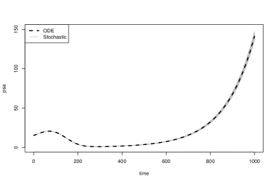
(a) ODE vs Stochastic, CAS policy

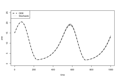
(b) ODE vs Stochastic, IAS policy

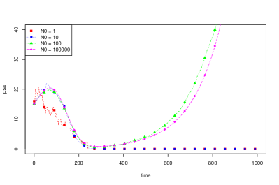
(c) CAS stochastic, $N_{0}$ varying

(d) IAS stochastic, external noise source

Figure 3: (3(a) and 3(b)) Comparison of simulated trajectories of PSA in the sCCP-programs and in the ODE models, both under CAS and IAS drug dispensation policies. Stochastic trajectories are generated by a Gillespie-like simulation algorithm [19]. The time unit is a day. Parameters of ODE are as in Figure 1. Scaling parameters of the stochastic model are set to $N_{0}=10^{5}$, $\Omega_{Z}=10^{5}$, $\Omega_{V}=10^{5}$. PSA of the stochastic model is rescaled as $v=\frac{V}{\Omega_{V}}$ before being plotted, so to have the same scale in both modes. Initial values of scaled variables are $x=15$, $y=0.1$, $z=12$. In the CAS policy, chemical castration is always in force. The IAS policy adopted is the following: every 4 weeks (28 time units) the value of PSA is checked. Drug dispensation is interrupted if normalized PSA has dropped below 4, while it is resumed when PSA exceeds 10. The behaviour of the stochastic model is essentially indistinguishable from the behavior of the ODE one. This basically happens for scaling parameters greater than $10^{3}$, hence their precise values do not have a relevant impact in the dynamics, as long as they are large enough. (3(c)) Comparison of single trajectories for CAS policy, and different values of $N_{0}$. (3(d)) Single trajectory for IAS policy in the presence of an external random disturbance source.

4.1 Hybrid dynamics and drug dispensation

The sCCP-program described above corresponds to the Continuous Androgen Suppression (CAS) policy [22, 12]. As said, more effective drug dispensation policies have been studied and in particular the Intermittent Androgen Suppression (IAS) has been proven effective to control prostate tumour development [4]. The mathematical rendering of such a policy calls naturally into play a hybrid model describing the on/off modes of drug dispensation. In our stochastic program this is done by introducing a variable $U$ (corresponding to the variable $u$ of the differential equation model) governing the switch between on/off androgen deprivation policy. The syntactic feature of $U$ is that it turns out to appear only in guards and not in rates: it is purely a control variable. More specifically, it appears in the new agent corresponding to androgen hormone production:

$$\mathtt{produceANDHc} [U=0\rightarrow Z^{\prime}=Z+1]_{\frac{z_{0}\Omega_{Z}}{\tau}}.\mathtt{produceANDHc}+[U=1\rightarrow Z^{\prime}=Z+1]_{0}.\mathtt{produceANDHc}$$ :-

The above agent replaces the corresponding agent ($\mathtt{produceANDH}$) in Figure 2.

Typical drug dispensation policies for androgen deprivation, control PSA concentration at fixed time intervals (usually every 4 weeks) and determine whether dispensation should be resumed/suspended by checking whether specific threshold values are reached. In order to describe such a policy, we can use sCCP agents with infinite rate and guards on system time, as described in Section 3. More precisely, we just need a variable $W$, which will describe in which day the level of PSA will be controlled, initially set to $\delta_{t}=28$, and add in parallel to the sCCP program the agent $\mathtt{checkPSA\_on}$, defined by:

$$\mathtt{checkPSA\_on} [Time=W\wedge V<v_{on}\rightarrow W^{\prime}=W+\delta_{t}\wedge U^{\prime}=0]_{\infty}.\mathtt{checkPSA\_off}$$ :-

$$+ [Time=W\wedge V\geq v_{on}\rightarrow W^{\prime}=W+\delta_{t}]_{\infty}.\mathtt{checkPSA\_on}$$

$$\mathtt{checkPSA\_off} [Time=W\wedge V\geq v_{off}\rightarrow W^{\prime}=W+\delta_{t}\wedge U^{\prime}=1]_{\infty}.\mathtt{checkPSA\_on}$$ :-

$$+ [Time=W\wedge V<v_{off}\rightarrow W^{\prime}=W+\delta_{t}]_{\infty}.\mathtt{checkPSA\_off}$$

Notice that, according to the semantics of Section 3, this is a proper hybrid model, as the explicit management of simulation time is a continuous ingredient. However, our semantics machinery in terms of TDSHA allows a much higher degree of flexibility, for instance treating (some of) the system variables as continuous to speed up simulation times.

5 Experimental results

In this section we briefly present an experimental analysis of the models of the previous section. More details on the analysis can be found in the supplementary material, available online [6]. The parameters are fixed to the same values of the ODE model (see Figure 1). The three scaling factors, $N_{0}$, $\Omega_{Z}$ and $\Omega_{V}$, have been fixed to values that we deemed meaningful and that were checked against real data, see the caption of Figure 3.

The first analysis that we consider is the comparison of the evolution of the agent-based stochastic model with the temporal evolution of ODE. In Figures 3(a) and 3(b) we compare the dynamics of PSA for the CAS and IAS drug dispensation policies, respectively. We show only the value of PSA, as it is the only observable quantity of the model. As we can see, the two models behave essentially in the same way. Even if a similar behaviour had to be expected, the fact that the stochastic system basically shows no noise at all may be seen as quite surprising. Actually, this phenomenon can be easily explained observing that the variables we are considering are all taking large values, i.e. they correspond to large populations, on the order of millions of cells or millions of molecules (in Figure 3, a PSA level of 10 corresponds to 1 million molecules). In these circumstances, the relative magnitude of fluctuations, which is of the order of $\frac{1}{\sqrt{N}}$, is too small to produce significant effects [18]. This essentially means that the variability in behaviour between single cells is lost when we consider large populations: the differences cancel out and the observed behaviour essentially coincides with the average one (cf. also Section 1 of Supplementary Material [6]).

One of the advantages of having a discrete and stochastic model is that we can also study the behaviour of the model when the population of cells is small. One way to perform this experiment in this setting is to decrement the parameter $N_{0}$, with the overall effect of reducing the total number of cancer cells. In Figure 3(d), we show the evolution of the number of tumour cells for different values of $N_{0}$. As expected, as $N_{0}$ decreases the evolution becomes more noisy. Interestingly, for very small populations the model changes its behaviour: there is a considerable probability that AI cells can extinguish before AD cells are eliminated by chemical castration, so that the tumour tends to be completely eliminated and no relapse can be observed. These low numbers may describe a situation during the initial stages of the tumour. Interestingly, the IAS therapy is less effective for low populations, as it reduces the chance of extinction of AD cells, so that the probability of tumour extinction is considearably lower. Details can be found in Section 2 of the Supplementary Material [6].

The sCCP-program model of tumor growth of Section 4 essentially does not show any noise in case of large cellular populations. Therefore, we considered possible modifications of the model to introduce some form of internal variability. This approach can be justified in order to check whether the variability in PSA concentration that is observed in real measurements, can be explained by the simple structure of this model. First, we modified the model adding a random source of variation in the PSA production rate. In Section 3 of the Supplementary Material [6] we present an experiment in which the production rate of PSA is no longer a constant with respect to the total number of tumor cells, but it is variable. In particular, we assume that production rate of PSA is a random number, uniformly distributed in the interval $[0,2\frac{\Omega_{V}(X+Y)}{N_{0}}]$. This is accomplished in the sCCP-program by introducing a new variable $K$ (the new production rate) and replacing the agent $\mathtt{producePSA}$ with the following one:

$$\mathtt{producePSA^{\prime}}\ \mbox{:-}\ [true\rightarrow K^{\prime}=Unif(0,2)]_{\infty}.[true\rightarrow V^{\prime}=V+1]_{K\frac{\Omega_{V}}{N_{0}}(X+Y)}.\mathtt{producePSA^{\prime}}.$$

Interestingly, even a large randomness in the PSA production rate does not result in a significant noisy behaviour: also in this case the fluctuations are averaged out.

We also considered a different modification of the model, in which we try to see whether noise may emerge as a consequence of the interaction with some external mechanism, possibly dependent on some global (physiological) condition. Specifically, we added a variable $H$ (for “hidden”) that can assume just two possible values, namely 0 and 1, representing the presence/absence of an unspecified (physiological) condition. We assume that $H$ switches from 0 to 1 and vice versa twice a day on average, and that the production rate of PSA is subject to a threefold increase when $H=1$. Hence, we added to the model the following agent:

$$\mathtt{hidden}\ \mbox{:-}\ [H=0\rightarrow H^{\prime}=1]_{2}+[H=1\rightarrow H^{\prime}=0]_{2},$$

and we replaced the PSA degradation rate by $(1+2H)$. Trajectories for this model are shown in Figure 3(d). In this case, we observe noise also in the case of large populations, cf. Section 4 of the Supplementary Material [6].

We stress that these last two models do not necessarily have any biologically significant interpretation. They are just illustrative examples of possible sources of noise in systems with large populations.

The analysis we carried out is different from the one of [30]. In this paper, noise is introduced in the model as an additional disturbance term in the ODEs (hence using Stochastic Differential Equations). In this case, however, the model does not provide any possible explanation of noise in terms of mechanisms intrinsic to the system under study. On the contrary, our study is aimed at better clarifying if the observed noise can be explained in terms of specific mechanisms, i.e. in terms of intrinsic properties of a given model. Notice that some noise will inevitably be introduced by factors external to the system, for instance by measurement errors.

What we understood from the analysis presented here is that the structure of phenomenological tumour cell growth models, like the one considered in this paper, may not be sufficiently rich to contain internal mechanisms for noise generation. If one is interested in these issues, then more complex models, taking into account more detailed biological mechanisms, should be considered. These models can also be easily described in our programming framework. We stress that this kind of analysis is more easily carried out in a discrete and stochastic setting.

6 Conclusion

The technique presented in this paper consists in showing how to step from a differential equation model to a “program” model, taking the form of a network of interacting agents. The specific programming language we used, allows us also to introduce a stochastic element (internal to the model and) rendered as the speed at which any specific interaction takes place. In particular, we considered a few extensions of sCCP-programs to describe time-driven events and random updates. General sCCP-programs, in addition, can easily model cell duplication events in the low level model of Section 2, by an unrestricted usage of parallel composition and local variable declaration. In general, communication between agents representing single cells can be easily encoded in an asynchronous setting like the one of sCCP  using dedicated variables, playing the role of communication channels, or modelling protein-mediated interaction. Exploiting the programmability of the shared memory (constraint store), one can easily introduce spatial information [10] or more complex cell interaction rules. Hence, sCCP-programs allow us to model explicitly geometrically qualified interactions or complex competitive dynamics regulating cells growths and deaths. However, a satisfactory definition of the hybrid semantics for this larger class of sCCP programs is still an open issue.

A programming environment like sCCP allows the construction of a “wizard” for fast prototyping of (cancer) cell population dynamics. Among other things, this approach should allow us to easily address such basic questions as the effect and nature of noise, parameter dependencies, logical structure of the interactions, etc. More advanced analysis techniques, like statistical model checking [23], will further enhance the framework.

We presented here a quantitative analysis on the nature of noise for a differential equation model of prostate cancer, based on the construction of an agent-based version of the model. Specifically, we showed that the phenomenological interactions of this model are not able to explain observed noise in data. We suggested that a more detailed description of interaction and regulation mechanisms involved is needed to better clarify the noise effects. We plan to further investigate this direction, taking also into account spatial organization of the tumour. Our future work will also benefit from a comparison with experimental data.

References

- [1]
- [2]
- [3] SBML website. http://www.sbml.org.
- [4] P.A. Abrahamsson (2010): Potential benefits of intermittent androgen suppression therapy in the treatment of prostate cancer: a systematic review of literature. Eur Urol 57, pp. 49–59, 10.1016/j.eururo.2009.07.049.
- [5] M. Bernardo & R. Gorrieri (1998): A tutorial on EMPA: a theory of concurrent processes with nondeterminism, priorities, probabilities and time. Theoret. Comput. Sci. 202, pp. 1 –54, 10.1016/S0304-3975(97)00127-8.
- [6] Supplementary Material. http://www.dmi.units.it/b̃ortolu/files/COMPMOD2011supp.pdf.
- [7] L. Bortolussi & A. Policriti (2008): Modeling Biological Systems in Concurrent Constraint Programming. Constraints 13(1), 10.1007/s10601-007-9034-8.
- [8] L. Bortolussi & A. Policriti (2009): Dynamical systems and stochastic programming — from Ordinary Differential Equations and back. T. Comp. Sys. Bio., XI pp. 216-267, 10.1007/978-3-642-04186-0_11.
- [9] L. Bortolussi & A. Policriti (2009): Hybrid Semantics of Stochastic Programs with Dynamic Reconfiguration. In: Proc. of CompMod, 10.4204/EPTCS.6.5.
- [10] L. Bortolussi & A. Policriti (2009): Tales of Spatiality in stochastic Concurrent Constraint Programming. In: Proc. of Bio-Logic.
- [11] L. Bortolussi & A. Policriti (2010): Hybrid Dynamics of Stochastic Programs. Theor. Comp. Sc. 411(20), pp. 2052-2077, 10.1016/j.tcs.2010.02.008.
- [12] M. K. Brawer (2006): Hormonal Therapy for Prostate Cancer. Rev Urol 8, pp. S35–S47.
- [13] F. Ciocchetta (2009): Bio-PEPA with Events. T. Comp. Sys. Bio. 11, pp. 45–68, 10.1007/978-3-642-04186-0_3.
- [14] F. Ciocchetta & J. Hillston (2008): Formal methods for computational systems biology, chapter Process algebras in systems biology, pp. 265–312. Springer-Verlag, 10.1007/978-3-540-68894-5_8.
- [15] F. Ciocchetta & J. Hillston (2009): Bio-PEPA: A framework for the modelling and analysis of biological systems. Theor. Comp. Sc. 410(33-34), pp. 3065 – 3084, 10.1016/j.tcs.2009.02.037.
- [16] M.H.A. Davis (1993): Markov Models and Optimization. Chapman & Hall.
- [17] M. Ajmone Marsan, G. Balbo, G. Conte, S. Donatelli & G. Franceschinis (1995): Modelling with Generalized Stochastic Petri Nets. Wiley.
- [18] D. Gillespie (2000): The chemical Langevin equation. Journal of Chemical Physics 113(1), pp. 297–306, 10.1063/1.481811.
- [19] D.T. Gillespie (1977): Exact Stochastic Simulation of Coupled Chemical Reactions. J. of Phys. Chem. 81(25), 10.1021/j100540a008.
- [20] H. Hermanns, U. Herzog & J.P. Katoen (2002): Process algebra for performance evaluation. Theor. Comp. Sci. 274(1-2), pp. 43–87, 10.1016/S0304-3975(00)00305-4.
- [21] A.M. Ideta, G. Tanaka, T. Takeuchi & K. Aihara (2008): A mathematical model of intermittent androgen suppression for prostate cancer. Nonlinear Science 18, pp. 593–614, 10.1007/s00332-008-9031-0.
- [22] T. L. Jackson (2004): A mathematical model of prostate tumor growth and androgen-independent relapse. Disc Cont Dyn Sys B 4, pp. 187–201, 10.3934/dcdsb.2004.4.187.
- [23] S.K. Jha, E.M. Clarke, C.J. Langmead, A. Legay, A. Platzer & P. Zuliani (2009): A Bayesian Approach to Model Checking Biological Systems. In: Proc. of the CMSB, pp. 218–234, 10.1007/978-3-642-03845-7_15.
- [24] P. Lecca, O. Kahramanogullari, D. Morpurgo, C. Priami & R. Soo (2011): Modelling the tumor shrinkage pharmacodynamics with BlenX. In: Proc. of ICCABS, 10.1109/UKSIM.2011.24.
- [25] T. Mazza & M. Cavaliere (2009): Cell Cycle and Tumor Growth in Membrane Systems with Peripheral Proteins. Electron. Notes Theor. Comput. Sci. 227, pp. 127–141, 10.1016/j.entcs.2008.12.108.
- [26] C.J. Mode (2005): Semi-Markov Processes. John Wiley & Sons, Ltd.
- [27] J. R. Norris (1997): Markov Chains. Cambridge University Press.
- [28] A.R. Rao, H.G. Motiwala & O.M.A. Karim (2008): The discovery of Prostate-Specific Antigen. BJU Int. 101, pp. 5–10, 10.1111/j.1464-410X.2007.07138.x.
- [29] D. Skulj (2009): Discrete time Markov chains with interval probabilities. Int. J. Approx. Reasoning 50(8), pp. 1314–1329, 10.1016/j.ijar.2009.06.007.
- [30] G. Tanaka, Y. Hirata, S.L. Goldenberg, N. Bruchovsky & K. Aihara (2010): Mathematical modelling of prostate cancer growth and its application to hormone therapy. Phyl Trans Royal Soc A 368, pp. 5029–5044, 10.1098/rsta.2010.0221.
- [31] D. J. Wilkinson (2006): Stochastic Modelling for Systems Biology. Chapman & Hall.