On the inclusive gluon production in the Lipatov effective action formalism

Abstract

The process of gluon production in quark-nucleus collisions is studied in the framework of Lipatov’s effective action formalism. The relevant simplifications and rules for longitudinal integrations are discussed in detail. The results obtained with the help of these rules correspond to the purely transversal formalism based on effective vertices in the transversal space.

1 Introduction

In the framework of the perturbative QCD, in the Regge kinematics, particle interaction can be described by the exchange of reggeized gluons which emit and absorb real gluons and also may split into several reggeized gluons. Emission of real gluons from reggeized gluons is described by vertices introduced in  [1] for non-split reggeons (”Lipatov vertices”) and in  [2] for split reggeons (”Bartels vertices”). Originally both type of vertices were calculated directly from the relevant simple Feynman diagrams in the Regge kinematics. Later a powerful effective action formalism was proposed by L.N.Lipatov  [3], which considers reggeized and normal gluons as independent entities from the start and thus allows to calculate all QCD diagrams in the Regge kinematics automatically and in a systematic and self-consistent way. However the resulting expressions are 4-dimensional and need reduction to the final 2-dimensional transverse form. This reduction is trivial for tree diagrams but becomes less trivial for diagrams with loops.

In the paper of two co-authors of the present paper (M.A.B. and M.I.V.)  [4] it was demonstrated that the diffractive amplitude for the production of a real gluon calculated by means of the Lipatov effective action and based on the Reggeon $\to$ one or two Reggeons and Particle (R$\to$R(R)P) vertices, after integration over longitudinal variables, goes over into the transversal expression obtained via the Lipatov and Bartels vertices (”BFKL-Bartels formalism”). However in the process of reduction to the transverse form a certain prescription had to be used to give sense to divergent integrals.

The total inclusive cross-section off the nucleus, apart from the diffractive contribution, contains a contribution from intermediate inelastic and possibly coloured states. This latter contribution has a structure different from the studied diffractive one. In particular, for the double scattering and in the lowest order, with which we limit ourselves here, a part of it is constructed as a square modulus of tree production amplitudes with the same R$\to$R(R)P vertices, so that the loops only appear at the stage of the formation of the cross-section itself. Correspondingly the longitudinal integrals which appear have a more complicated structure as compared to the diffractive contribution. In this paper we study this part of the non-diffractive contribution. We show that after integration over longitudinal variables it also coincides with the result obtained with the help of Lipatov and Bartels vertices directly in the transverse space  [5] provided a certain part of the R$\to$RRP vertex is dropped. This part was demonstrated to be absent in a particular kinematics, relevant for the inclusive cross-section  [6]. Our result confirms that the restoration of the unitarity contribution from the triple discontinuity of the amplitude, which can be proven for the total cross-section, remains valid also for the inclusive cross-section.

Note that a second part of the non-diffractive contribution corresponds to the product of tree amplitudes and amplitudes with a loop. The study of this ’single cut’ contribution requires knowledge of a more complicated R$\to$RRRP vertex and is postponed for future publications.

In our derivation we use a simplified picture, in which both incident and target particles are quarks. Also, we restrict ourselves to the double scattering and lowest non-trivial order of perturbation expansion.

2 Inclusive production off the nucleus

We start with reviewing the Glauber picture of gluon production off the nucleus of atomic number $A$ coming from the double scattering on the nuclear components. This derivation closely follows the original one in [7] (see also a later presentation in  [8]). There one can find a detailed description of the separation of the nuclear part, which is briefly repeated in the following. Our specific goal is to pass to light-cone variables and c.m. system for the high-energy part and find the kinematical region of momenta relevant for the calculation of the inclusive cross-section. The corresponding diagram is shown in Fig. 1. The blob $H$ corresponds to the high-energy part. The part belonging to the nucleus is indicated by nucleon propagators attached to the high-energy blob. For the inclusive cross-section the blob $H$ is to be cut in the center but this is not shown, since in fact we have to take its imaginary part above the cut corresponding to the variable $M^{2}=(k+l_{1}+l_{2}-p)^{2}>0$ having the meaning of the missing mass squared for gluon production. So we may start from the blob itself.

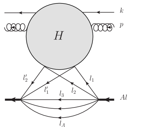
Figure 1: Inclusive production off the nucleus

Separation of the nuclear part is standardly done in the nuclear rest system (lab. system), in which the total nucleus 3-momentum $A{\bf l}$ is zero. Individual nuclear momenta have their components

$$l_{i}=l+\lambda_{i},\ \ l^{\prime}_{i}=l+\lambda^{\prime}_{i},\ \ l=(m-\epsilon,\vec{0}),$$ (1)

where $m$ is the nucleon mass, $\epsilon\to 0$ the binding energy per nucleon and where $\lambda_{i}=\lambda^{\prime}_{i}$ for $i\geq 3$. In the nucleus $\lambda_{i0}\sim\epsilon$ and $\lambda_{iz}\sim\lambda_{i\perp}\sim\sqrt{m\epsilon}$. So $|\lambda_{i0}|<<|\vec{\lambda}_{i}|<<l_{0}$ and similarly for the primed momenta.

Now we turn to the high-energy blob $H$. It is a Lorenz invariant function of nuclear momenta depending on $\lambda^{2}$ and products $kl_{1},kl_{2},k\lambda$ and $pl_{1},pl_{2},p\lambda$ where $\lambda=l^{\prime}_{1}-l_{1}=l_{2}-l^{\prime}_{2}$. In the lab. system we find $kl_{1}\simeq kl_{2}\simeq kl$, $pl_{1}\simeq pl_{2}\simeq pl$ and do not depend on nuclear momenta at all. The only dependence comes from $k\lambda$, $p\lambda$ and $\lambda^{2}$. Taking into account that $\lambda_{0}<<\lambda_{z}\to 0$ and that $k_{\perp},p_{\perp}<<k_{z},p_{z}\to\infty$ we find that in fact the only relevant variables are

$$k\lambda=-k_{z}\lambda_{z},\ \ p\lambda=-p_{z}\lambda_{z},$$ (2)

so that the high-energy part depends only on $\lambda_{z}$ via $(k\lambda)$ and $(p\lambda)$: $H=H(\lambda_{z})=H(p\lambda,k\lambda)$.

The separation of the nuclear part then easily follows. We have $(A-1)$ independent nuclear momenta, which may be chosen in a different manner. First we perform integrations over zero-components, taking as independent variables $\lambda_{20},\lambda^{\prime}_{20},\lambda_{i0},\ \ i\geq 3$. Integration over $\lambda_{i0},\ \ i\geq 3$ is done automatically when we take the cut, which puts these nucleons on the mass-shell. The dependence on $\lambda_{20}$ and $\lambda^{\prime}_{20}$ is assumed to be contained in four propagators for the active nucleons 1 and 2. The vertex for the decomposition of the nucleus as a whole into free nucleons is assumed to be independent of zero-components, which physically corresponds to absence of essential retardation in the nucleon-nucleon potentials. Then integration over $\lambda_{20}$ and $\lambda^{\prime}_{20}$ is done trivially and gives two denominators, which together with the above mentioned vertex form the product of nuclear wave functions in the momentum space

$$\frac{1}{2}A(A-1)\frac{(2\pi)^{3}}{m}\psi({\bf l}_{1},{\bf l}_{2},...{\bf l}_{A})\psi^{*}({\bf l}^{\prime}_{1},{\bf l}^{\prime}_{2},...{\bf l}^{\prime}_{A}),$$ (3)

(the coefficient is easily determined from the comparison with the baryonic nuclear form-factor at zero transferred momenta). Integration over the 3-momenta of spectator nucleons 3,…A converts this into the density matrix for the two active nucleons

$$\frac{1}{2}A(A-1)\frac{(2\pi)^{3}}{m}\rho({\bf l}_{1},{\bf l}_{2}|{\bf l}^{\prime}_{1},{\bf l}^{\prime}_{2}).$$ (4)

Next step is integration over the transverse momenta of the active nucleons $l_{1\perp},l_{2\perp},l^{\prime}_{1\perp}$ and $l^{\prime}_{2\perp}$ with

$$l_{1\perp}+l_{2\perp}=l^{\prime}_{1\perp}+l^{\prime}_{2\perp}.$$ (5)

The high-energy part is independent of these transverse momenta. We present

$$2\pi\delta^{2}(l_{1\perp}+l_{2\perp}-l^{\prime}_{1\perp}-l^{\prime}_{2\perp})=\int\frac{d^{2}b}{2\pi}e^{ib(l_{1\perp}+l_{2\perp}-l^{\prime}_{1\perp}-l^{\prime}_{2\perp})}$$ (6)

and pass to the transverse coordinate space in the density matrix. We get (suppressing the dependence on $z$-components)

$$\frac{1}{(2\pi)^{9}}\int\prod_{i=1,2}d^{2}l_{i}d^{2}l^{\prime}_{i}\prod_{i=1,2}d^{2}x_{i}d^{2}x^{\prime}_{i}d^{2}be^{ib(l_{1\perp}+l_{2\perp}-l^{\prime}_{1\perp}-l^{\prime}_{2\perp})}$$

$$e^{-ix_{1}l_{1\perp}-ix_{2}l_{2\perp}+ix^{\prime}_{1}l^{\prime}_{1\perp}+ix^{\prime}_{2}l^{\prime}_{2\perp}}\rho(x_{1},x_{2}|x^{\prime}_{1},x^{\prime}_{2})=\int\frac{d^{2}b}{2\pi}\rho(b,b|b,b).$$ (7)

We are left with integrations over the $z$-components $l_{1z},l_{2z}$ and $\lambda_{z}$ with the high-energy part depending only on $\lambda_{z}$. So our expression for the amplitude is

$${\cal A}=A(A-1)\frac{(2\pi)^{3}}{2m}\int\frac{d^{2}bdl_{1z}dl_{2z}d\lambda_{z}}{(2\pi)^{4}}H(\lambda_{z})\rho(b,l_{1z};b,l_{2z}|b,l_{1z}+\lambda_{z};b,l_{2z}-\lambda_{z}).$$ (8)

Again we pass to the coordinate representation for the density matrix as a function of $z$-components of momenta to obtain

$${\cal A}=\frac{A(A-1)}{4\pi m}\int d^{2}bd\lambda_{z}H(\lambda_{z})dz_{1}dz_{2}e^{i\lambda_{z}(z_{1}-z_{2})}\rho(b,z_{1};b,z_{2}|b,z_{1};b,z_{2}).$$ (9)

This is our final expression. Integration over $z_{1}-z_{2}$ is carried out along the path passing through the nucleus of the average length $\sim R_{A}\sim A^{1/3}$ and large in the limit $A>>1$. Correspondingly the order of essential values of $\lambda_{z}$ is $\sim A^{-1/3}$. Taking the imaginary part we obtain the inclusive cross-section as

$$\frac{(2\pi)^{3}d\sigma}{d^{3}p}=\frac{1}{s}{\rm Im}\,{\cal A}=\frac{A(A-1)}{4\pi ms}\int d^{2}bd\lambda_{z}{\rm Im}\,H(\lambda_{z})dz_{1}dz_{2}e^{i\lambda_{z}(z_{1}-z_{2})}\rho(b,z_{1};b,z_{2}|b,z_{1};b,z_{2}).$$ (10)

In fact the high-energy part normally contains a pole at $\lambda_{z}=0$  [7, 8], so that its imaginary part can be presented as

$${\rm Im}\,H(\lambda_{z})=F\delta(\lambda_{z})+C(\lambda_{z}).$$ (11)

The term with $\delta(\lambda_{z})$ gives the standard Glauber contribution corresponding to multiple collisions of the incident particle on the nucleons located at large distances between one another. Integration over $\lambda_{z}$ gives :

$$\frac{(2\pi)^{3}d\sigma}{d^{3}p}=\frac{A(A-1)}{4\pi ms}F\int d^{2}bdz_{1}dz_{2}\rho(b,z_{1};b,z_{2}|b,z_{1};b,z_{2}).$$ (12)

If we neglect nuclear correlations and factorize the density matrix (12) transforms into the standard Glauber expression

$$\frac{(2\pi)^{3}d\sigma}{d^{3}p}=\frac{A(A-1)}{4\pi ms}F\int d^{2}bT^{2}(b),$$ (13)

where $T_{A}(b)$ is the standard nuclear profile function

$$T(b)=\int dz\rho(b,z).$$ (14)

For $A>>1$ this Glauber contribution has order $A^{4/3}$. The non-singular part $C(\lambda_{z})$ gives a contribution corresponding to the scattering of the incident particle on two nucleons located at the same point. Indeed at $\lambda_{z}\to 0$ one can take $C(\lambda_{z})$ out of the integration over $\lambda_{z}$ in (9), so that this integration gives $2\pi\delta(z_{1}-z_{2})$. At $A>>1$ the resulting contribution has order $A$ and and can be neglected as compared to (12). So the leading Glauber term is determined by the contribution to $H(\lambda_{z})$ singular in the limit $\lambda_{z}\to 0$.

In fact we shall find out that the situation is more complicated. Many of our contributions to Im $H(\lambda_{z})$ will contain terms proportional to $\delta(\lambda_{z}-\beta(q_{\perp}))$ under the sign of integration over transverse momentum $q_{\perp}$ of the exchanged reggeons. In the limit when the energies of both the projectile and observed gluon tend to infinity all $\beta$ tend to zero, so that one finally obtains a non-zero contribution to the Glauber cross-section. However one finds that $\beta$ diminishes either with the energy of the projectile or with the energy of the observed gluon, much smaller than the former:

$$\beta(q_{\perp})\sim\frac{mq_{\perp}^{2}}{s}\ \ {\rm or}\ \ \beta(q_{\perp})\sim\frac{mq_{\perp}^{2}}{xs}$$

with $x=p_{+}/k_{+}<<1$. Put in (10) this introduces an oscillating factor into the integrand

$$e^{(z_{1}-z_{2})\frac{mq_{\perp}^{2}}{s}}\ \ {\rm or}\ \ e^{(z_{1}-z_{2})\frac{mq_{\perp}^{2}}{sx}}.$$

At very large $s$ this factor turns to unity. This happens when

$$R_{A}\frac{mq_{\perp}^{2}}{xs}<<1.$$ (15)

In the following we shall assume that this condition is fulfilled. Then we can neglect all terms depending on the transverse momenta as compared to $\lambda$ in the integrands. In particular we can neglect $p_{-}=-p_{\perp}^{2}/2p_{+}$ where it enters with $\lambda_{-}=-\lambda_{z}/\sqrt{2}$ and integration variables.

Function $H(\lambda_{z})=H(p\lambda,k\lambda)$ can be calculated in any system and in the c.m. system $k_{z}+l_{z}=k_{\perp}=l_{\perp}=0$ in particular, using the fact that the relevant scalar products are Lorenz invariant. For the calculation it is instructive to see the relative orders of all scalar product on which $H$ depends. They are $(kp),(kl),(pl),(k\lambda)$ and $(p\lambda)$. We define the longitudinal momenta as $a_{\pm}=a_{0}\pm a_{z}$. In the lab. system, denoting the $\pm$ momenta with tildes, we have $\tilde{l}_{\pm}=m$, $\tilde{\lambda}_{\pm}=\mp\lambda_{z}$, so that $\lambda_{-}=-\lambda_{z}(\sqrt{s}/m)$ The total energy squared is $s=2(kl)=k_{+}l_{-}=\tilde{k}_{+}m$, from which we find $\tilde{k}_{+}=s/m$ and then $\tilde{p}_{+}=xs/m$. We also have $\tilde{k}_{-}=0$ and $\tilde{p}_{-}-mp_{\perp}^{2}/xs$. Furthermore

$$s_{1}=(k+p)^{2}=2(kp)=k_{+}p_{-}=-\frac{p_{\perp}^{2}}{x},\ \ s_{2}=(p+l)^{2}=p_{+}l_{-}=xs,$$ (16)

(as expected $s_{1}s_{2}=-p_{\perp}^{2}s$). We assume all the three $s,s_{1}$ and $s_{2}$ large, which requires $x<<1$. Using the order of $\lambda_{z}$ in the lab system we find $\lambda_{\perp}=0$ so that $kq=\sim s\sqrt{\frac{\epsilon}{m}}$ and $pq=\sim xs\sqrt{\frac{\epsilon}{m}}$ So we have relative orders

$$\frac{k\lambda}{kl}\sim\sqrt{\frac{\epsilon}{m}},\ \ \frac{k\lambda}{pl}\sim\frac{1}{x}\sqrt{\frac{\epsilon}{m}},\ \ \frac{k\lambda}{k\lambda}\sim\frac{sx}{p_{\perp}^{2}}\sqrt{\frac{\epsilon}{m}},\ \ \frac{p\lambda}{kl}\sim x\sqrt{\frac{\epsilon}{m}},\ \ \frac{p\lambda}{pl}\sim\sqrt{\frac{\epsilon}{m}},\ \ \frac{p\lambda}{kp}\sim\frac{s}{p_{\perp}^{2}}\sqrt{\frac{\epsilon}{m}}.$$ (17)

In all cases the limit $\lambda_{z}\to 0$ is obtained taking $\epsilon/m\to 0$ and therefore neglecting $(k\lambda)$ and $(p\lambda)$ as compared to $(kl),(pl)$ and $(kp)$.

This fixes the rules for calculating the high-energy part $H$. Assuming for simplicity that the nucleus consists of quarks, one can take the two initial target quark momenta equal to $l$, the two final momenta of the target quark as $l+\lambda$ and $l-\lambda$ with $\lambda_{\perp}=\lambda_{+}=0$. Under assumption (15) one can neglect all terms depending on the transverse momenta ( $p_{-}$ in particular) as compared to $\lambda_{-}$ and “-”-components of integration momenta. Since these terms contain $k_{+}$ or $p_{+}$ in the denominator, this also corresponds to taking the limit $k_{+},p_{+}\to\infty$ in the final formulas. Then one has to take the limit $\lambda\to 0$ leaving only terms singular in this limit.

3 Non-diffractive contribution to the inclusive gluon production from R$\to$R(R)P vertices: the diagrams

In the framework of the effective action [3], in the lowest order the non-diffractive inclusive cross-section on two scattering centers (”nucleons”) generated by the R$\to$R(R)P vertices is given by the square modulus of the sum of five production amplitudes, shown in Fig. 2 and denoted as A,B,C,D and E. In the first four the number of reggeons does not change and the gluon is emitted by the R$\to$RP vertex. In Fig. 2,E the number of reggeons changes and the gluon is emitted by the R$\to$RRP vertex. In the kinematical region $q_{1-},q_{2-}\sim\lambda_{-}>>p_{-}$ essential for the inclusive cross-section, the diagrams A$-$D give only contributions to the production amplitude proportional to $\delta(q_{1-})$ or $\delta(q_{2-})$ and the diagram E contributes the rest  [6]. However, alternatively one can include diagrams A$-$D as a whole but then one has to exclude a part of the contribution from diagram E containing the principal part of the pole contribution at $q_{1,2-}=0$  [6]. We shall use the latter approach and discuss this point in the next section.

Taking the square modulus of the sum of these production amplitudes gives rise to 25 scattering amplitudes cut in the center, which are shown in Figs. 3–7. For interference diagrams only half is shown, the other half given by their complex conjugates. Note that the total contribution of these amplitudes to the cross-section includes also discontinuities across other cuts passing through only one of both targets. They involve the R$\to$RRRP vertex and, as mentioned in the Introduction, will be considered in a separate publication.

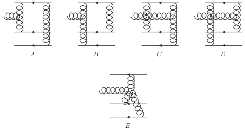
Figure 2: Gluon production amplitudes off two targets

As mentioned, for simplicity we model the two nuclear components by a pair of quarks or a pair of quark and antiquark with momenta $l_{1}$ and $l_{2}$ over which one has to integrate with the nuclear wave functions. Both $qq$ and $q\bar{q}$ targets lead to the same result. Here we will consider factors general for all these diagrams.

We choose $q_{1}$, $q_{1}^{{}^{\prime}}$, $l_{1}$ and $l_{1}^{{}^{\prime}}$ as integration variables. In the following we define (see Figs. 3–7 for notations)

$$\lambda=l_{1}^{{}^{\prime}}-l_{1}=l_{2}-l_{2}^{{}^{\prime}},\ \ q_{1}^{{}^{\prime}}=q_{1}-\lambda,\ \ q_{2}^{{}^{\prime}}=q_{2}+\lambda,\ \ q=p+q_{1}+q_{2}$$ (18)

with $\lambda_{+}=\lambda_{\perp}=0$.

We work in the Regge kinematics, so that the longitudinal components of our momenta should obey:

$$k_{+}\gg p_{+}\sim q_{+}\gg l_{1+}\sim l_{2+}\sim l^{\prime}_{1+}\sim l^{\prime}_{2+}\sim q_{1+}\sim q_{2+}\sim q^{\prime}_{1+}\sim q^{\prime}_{2+},$$ (19)

$$l_{1-}\sim l^{\prime}_{-}\sim l_{2-}\sim l^{\prime}_{2-}\gg p_{-}\sim q_{1-}\sim q_{2-}\sim q^{\prime}_{1-}\sim q^{\prime}_{2-}\gg k_{-}\sim q_{-}.$$ (20)

The quark masses are assumed to be equal to zero and we can put $k_{-}=k_{\perp}=l_{i+}=l_{i\perp}=0$ for $i=1,2$ Each transversal momentum is assumed to be much smaller than the larger of the longitudinal one.

Factors corresponding to the two target quarks, projected onto colourless states, are

$$2\pi\frac{g^{2}}{2N_{c}}l_{1-}^{2}\delta((l_{1}+q_{1})^{2})\ \ {\rm and}\ \ 2\pi\frac{g^{2}}{2N_{c}}l_{2-}^{2}\delta((l_{2}+q_{2})^{2})$$ (21)

We are interested in terms singular in $\lambda_{-}$.

The total number of longitudinal integrations is, obviously, four. However three of them are removed by the mass-shell conditions for real particles:

$$(k-q)_{-}=-\frac{q_{\perp}^{2}}{(k-q)_{+}},\ \ (l_{1}+q_{1})_{+}=-\frac{q_{1\perp}^{2}}{(l_{1}+q_{1})_{-}},\ \ (l_{2}+q_{2})_{+}=-\frac{q_{2\perp}^{2}}{(l_{2}+q_{2})_{-}}.$$ (22)

The last two conditions fix $q_{1+}$ and $q_{2+}$. From the first we find $q_{-}$ and from this relate $q_{1-}+q_{2-}=(q-p)_{-}\simeq-p_{-}$ We also have $q^{\prime}_{1}=l_{1}+q_{1}-l^{\prime}_{1}$ and $q^{\prime}_{2}=l_{2}+q_{2}-l^{\prime}_{2}$ and the emitted gluon momenta are (from the right) $q-q_{1}$, $q-q_{1}-q_{2}=p$ and $q-q_{1}-q_{2}+q^{\prime}_{1}$. Thus we are left with a single longitudinal variable for which we choose $q_{1-}$. So in our formulas momentum integrations are:

$$\frac{4}{(2\pi)^{8}k_{+}l_{-}^{2}}\int d^{2}q_{1\perp}d^{2}q_{2\perp}dq_{1-}\frac{1}{q_{1\perp}^{4}q_{2\perp}^{4}},$$ (23)

where we used that in our kinematics $l_{1-}=l_{2-}=l_{-}/2=\sqrt{s}/2$, $q^{\prime}_{1\perp}=q_{1\perp}$ and $q^{\prime}_{2\perp}=q_{2\perp}$.

4 Contribution from the R$\to$RRP vertex (diagram Fig. 3)

We start with the diagram in Fig. 3, which comes from the product of production amplitudes $(E)\cdot(E)^{*}$

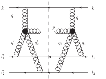
Figure 3: Contribution from two R$\to$RRP vertices

The product of reggeon propagators (apart from those included into the weight) in our approximation reduces to $1/q^{4}_{\perp}$. It depends only on the transversal components. The factor corresponding to the projectile quark $k$ is:

$$2\pi g^{2}\delta((k-q)^{2})k_{+}^{2}.$$ (24)

The R$\to$RRP vertex $q\to q_{1}+q_{2}+p$ was derived in [4]. It consists of two parts:

$$V=V_{1}+V_{2},$$ (25)

where

$$V_{1}=ig^{2}\frac{f^{ab_{1}d}f^{b_{2}cd}}{(q-q_{1})^{2}+i0}\Big{\{}q_{+}(q,\epsilon^{*}_{\perp})-\frac{q_{\perp}^{2}}{q_{1-}}\Big{[}(q-q_{1},\epsilon^{*}_{\perp})-\frac{(q-q_{1})^{2}}{p_{\perp}^{2}}(p,\epsilon^{*}_{\perp})\Big{]}\Big{\}}$$ (26)

and

$$V_{2}=ig^{2}\frac{f^{ab_{2}d}f^{b_{1}cd}}{(q-q_{2})^{2}+i0}\Big{\{}q_{+}(q,\epsilon^{*}_{\perp})-\frac{q_{\perp}^{2}}{q_{2-}}\Big{[}(q-q_{2},\epsilon^{*}_{\perp})-\frac{(q-q_{2})^{2}}{p_{\perp}^{2}}(p,\epsilon^{*}_{\perp})\Big{]}\Big{\}}.$$ (27)

It is convenient to split the terms in each of the parts $V_{1}$ and $V_{2}$ into two terms depending on their singularities in $q_{1-}$ and $q_{2-}$ respectively. Take $V_{1}$. In the second term in the brackets we present the product $1/q_{1-}[(q-q_{1})^{2}+i0]$ as

$$\frac{1}{q_{1-}[(q-q_{1})^{2}+i0]}=-\frac{1}{q_{+}a}\Big{(}\frac{1}{q_{1-}-a-i0}-\frac{1}{q_{1-}}\Big{)}=\frac{1}{a[(q-q_{1})^{2}+i0]}+\frac{1}{q_{1-}(q-q_{1})_{\perp}^{2}},$$

where

$$a=(q-q_{1})_{\perp}^{2}/q_{+}.$$ (28)

Combining terms with the same singularity in $q_{1-}$ we find

$$V_{1}=W_{1}+R_{1},$$ (29)

where

$$W_{1}=ig^{2}\frac{q_{+}q_{\perp}^{2}}{(q-q_{1})^{2}+i0}{\bf B}(p,q_{2},q_{1}){\bf e}_{\perp}f^{ab_{1}d}f^{b_{2}cd}$$ (30)

and

$$R_{1}=-ig^{2}\frac{q_{\perp}^{2}}{q_{1-}}{\bf L}(p,q_{2}){\bf e}_{\perp}f^{ab_{1}d}f^{b_{2}cd}.$$ (31)

Here the transverse spatial vectors ${\bf B}$ and ${\bf L}$ are the Bartels and Lipatov vertices respectively:

$${\bf L}(p,q_{2})=\frac{{\bf p}}{p_{\perp}^{2}}-\frac{{\bf p}+{\bf q}_{2}}{(p+q_{2})_{\perp}^{2}},\ \ \ {\bf B}(p,q_{2},q_{1})={\bf L}(p+q_{2},q_{1})$$ (32)

and we use $q-q_{1}=p+q_{2}$. Production amplitudes corresponding to the two terms $W_{1}$ and $R_{1}$ are schematically illustrated in Fig. 4. A similar representation for $V_{2}$ is obtained by interchanging the target quarks.

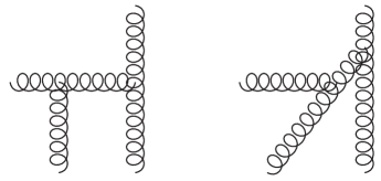
Figure 4: Two parts $W$ and $R$ of the R$\to$RRP vertex

As mentioned, the study of the production amplitude in the framework of the effective action and in the kinematics $q_{1,2-}>>p_{-}$ demonstrates that to get its correct parts, symmetric and antisymmetric with respect to the change $q_{1}\leftrightarrow q_{2}$, one should drop the contribution of $R_{1,2}$ but include diagrams A,$...$,D  [6]. So considering the contribution from the R$\to$RRP vertex we restrict ourselves to the contribution from from $W_{1,2}$ only.

Taking the square modulus, this contribution is a sum four parts, symbolically

$$(W_{1})\cdot(W_{1})^{*}+(W_{2})\cdot(W_{2})^{*}+(W_{1})\cdot(W_{2})^{*}+(W_{2})\cdot(W_{1})^{*}.$$ (33)

Obviously, the second term is obtained from the first one and the fourth term from the third one by the interchange $\lambda\to-\lambda$. So it is sufficient to calculate $(W_{1})\cdot(W_{1})^{*}$ and $(W_{1})\cdot(W_{2})^{*}$.

Different parts carry different color factors. Combining with (27) the total color factor for the part $(W_{1})\cdot(W_{1})^{*}$ is

$$C_{11}=\frac{N^{2}_{c}-1}{8N_{c}}.$$ (34)

For the part $(W_{1})\cdot(W_{2}^{*})$ it is twice smaller:

$$C_{12}=\frac{N_{c}^{2}-1}{16N_{c}}.$$ (35)

1. $(W_{1})\cdot(W_{1})^{*}$

Neglecting the dependence on $q_{1-}$ of the target, the remaining dependence comes from the denominators of the two virtual gluon propagators

$$D_{1}=(q-q_{1})^{2}+i0$$ (36)

and

$$D_{2}=(q-q^{\prime}_{1})^{2}-i0=(q-q_{1}+\lambda)^{2}-i0.$$ (37)

The integral over the longitudinal variable is

$$I_{11}=\int dq_{1-}\frac{1}{((q-q_{1})^{2}+i0)((q-q_{1}+\lambda)^{2}-i0)}=I(-q,-q-\lambda).$$ (38)

Here for future use we define

$$I(p_{1},p_{2})=\int dq_{1-}\frac{1}{((q_{1}+p_{1})^{2}+i0)((q_{1}+p_{2})^{2}-i0)}=$$

$$=\frac{1}{p_{1+}p_{2+}}\int dq_{1-}\frac{1}{\Big{(}q_{1-}+p_{1-}+\frac{(q_{1}+p_{1})_{\perp}^{2}}{p_{1+}}+i0\cdot p_{1+}\Big{)}\Big{(}q_{1-}+p_{2-}+\frac{(q_{1}+p_{2})_{\perp}^{2}}{p_{2+}}-i0\cdot p_{2+}\Big{)}}\ .$$ (39)

When $p_{1+}p_{2+}>0$ in (39), the two poles in $q_{1-}$ lie on the opposite sides of the real axis. Taking the residue we find

$$I(p_{1},p_{2})=\frac{2\pi i}{p_{1+}p_{2+}}\cdot\frac{-{\rm sign}(p_{1+})}{p_{2-}-p_{1-}+\frac{(q_{1}+p_{2})_{\perp}^{2}}{p_{2+}}-\frac{(q_{1}+p_{1})_{\perp}^{2}}{p_{1+}}-i0\cdot{\rm sign}(p_{1+})}\ .$$ (40)

When $p_{1+}p_{2+}<0$, the two poles in $q_{1-}$ lie on the same side of the real axis and the integral equals to zero.

For (38) we use $q^{\prime}_{1\perp}=q_{1\perp}$, so $(q-q_{1})_{\perp}^{2}=(q-q^{\prime}_{1})_{\perp}^{2}$, and also assume (as always in the Regge kinematics) $q_{-}<<q_{1-}$, then

$$I_{11}=I(-q,-q-\lambda)=\frac{2\pi i}{q_{+}^{2}}\frac{1}{-\lambda_{-}+i0}.$$ (41)

The result has a pole at $\lambda_{1}=0$ and will give a non-zero contribution to the inclusive cross-section.

2. $(W_{1})\cdot(W_{2})^{*}$

The difference from the term $(W_{1})(W_{1})^{*}$ is in $D_{2}$, which is now changed to

$$D_{2}=(p+q^{\prime}_{1})^{2}-i0=(p+q_{1}-\lambda)^{2}-i0.$$ (42)

We get an integral

$$I_{12}=I(-q,p-\lambda)=0,$$ (43)

which is equal to zero since both poles are located in the upper half-plane.

3.

The total contribution from $W_{1,2}$ is given by the sum $(W_{1})\cdot(W_{1})^{*}+(\lambda\to-\lambda)$. We find

$$(W_{1})\cdot(W_{1})^{*}+(\lambda\to-\lambda)=4\pi^{2}\delta(\lambda_{-})q_{\perp}^{4}{\bf B}^{2}(p,q_{2},q_{1}).$$ (44)

Supplying all the rest factors and using the relation between $\lambda_{-}$ in the c.m. system and $\lambda_{z}$ in the lab. system we get for the factor $F$ in the high-energy part coming from the product $|(W)_{1}+(W)_{2}|^{2}$

$$F_{1}=4\pi msg^{10}\frac{N_{c}^{2}-1}{N_{c}}\int\frac{d^{2}q_{1\perp}d^{2}q_{2\perp}}{(2\pi)^{4}}\frac{1}{q^{4}_{1\perp}q^{4}_{2\perp}}{\bf B}^{2}(p,q_{2},q_{1}).$$ (45)

This is the same expression which follows in the purely transversal BFKL-Bartels approach.

5 Contributions from the R$\to$RP vertex

This contribution comes from the diagrams in which the number of reggeons does not change and the gluons are emitted by the Lipatov verices. It is generated by the square modulus of the sum of production amplitudes $(A)+(B)+(C)+(D)$ in Fig. 2). It can be split into a direct part $\sum$(I)$\cdot$(I)^∗, $I=A,B,C,D$ and the interference part $\sum$(I)$\cdot$(J)^∗, $I\neq J=A,B,C,D$. The factor corresponding to the projectile quark $k$ is $2\pi g^{4}\delta((k-q)^{2})k_{+}^{4}$.

5.1 The direct part

Diagrams corresponding to products $(A)\cdot(A)^{*}$ and $(C)\cdot(C)^{*}$ are shown in Fig. 5. The other two corresponding to products $(B)\cdot(B)^{*}$ and $(D)\cdot(D)^{*}$ are obtained by the interchange of target quarks 1 and 2, which reduces to the change $\lambda\to-\lambda$. So they need not be studied separately.

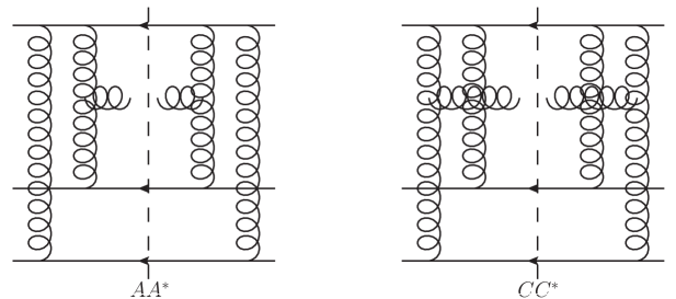
Figure 5: Direct diagrams with two R$\to$RP vertices

1. $(A)\cdot(A)^{*}$

The product of reggeon propagators and R$\to$RP vertices, summed over polarizations of the observed gluon, gives

$$g^{2}f^{a_{1}b_{1}c}f^{a^{\prime}_{1}b^{\prime}_{1}c}{\bf L}(p,q_{1}){\bf L}(p,q^{\prime}_{1}),$$ (46)

where vector ${\bf L}$ is the Lipatov vertex (32).

The colour factor is found to be

$$C_{AA}=\frac{(N_{c}^{2}-1)^{2}}{16N_{c}^{3}}.$$ (47)

The dependence on $q_{1-}$ comes from the virtual quarks propagators with the denominators

$$D_{1}=(k-q_{2})^{2}+i0=(k+p-q+q_{1})^{2}+i0$$ (48)

and

$$D_{2}=(k-q_{2}^{\prime})^{2}-i0=(k+p-q+q_{1}-\lambda)^{2}-i0.$$ (49)

Integration over $q_{1-}$ gives

$$I_{AA}=I(k+p-q,k+p-q-\lambda)=\frac{2\pi i}{k_{+}^{2}}\frac{1}{\lambda_{-}+i0},$$ (50)

where the relation $q^{\prime}_{2\perp}=q_{2\perp}$ is used.

2. $(C)\cdot(C)^{*}$

The reggeon propagators and vertices are obtained from (46) by the change $q_{1},b_{1}\to q_{2},b_{2}$ and $q^{\prime}_{1},b^{\prime}_{1}\to q^{\prime}_{2},b^{\prime}_{2}$. The dependence on $q_{1-}$ comes from the denominators in the virtual quarks propagators:

$$D_{1}=(k-p-q_{2})^{2}+i0=(k-q+q_{1})^{2}+i0,$$ (51)

$$D_{2}=(k-p-q_{2}^{\prime})^{2}-i0=(k-q+q_{1}-\lambda)^{2}-i0.$$ (52)

We get the longitudinal integral

$$I_{CC}=I(k-q,k-q-\lambda)=\frac{2\pi i}{k_{+}^{2}}\frac{1}{\lambda_{-}+i0}.$$ (53)

3.

Taking into account that the contributions from $(B)\cdot(B)^{*}$ and $(D)\cdot(D)^{*}$ are obtained from those from $(A)\cdot(A)^{*}$ and $(C)\cdot(C)^{*}$ respectively by the change $\lambda\to-\lambda$ we find

$$(A)\cdot(A)^{*}+(B)\cdot(B)^{*}=8\pi g^{10}l_{1-}l_{2-}k_{+}\frac{(N_{c}^{2}-1)^{2}}{N_{c}^{3}}\delta(\lambda_{-})\int\frac{d^{2}q_{1\perp}d^{2}q_{2\perp}}{(2\pi)^{4}}\frac{1}{q^{4}_{1\perp}q^{4}_{2\perp}}{\bf L}^{2}(p,q_{1}).$$ (54)

The contribution from $(C)\cdot(C)^{*}+(D)\cdot(D)^{*}$ is obtained from (54) by interchanging $q_{1\perp}\leftrightarrow q_{2\perp}$. So we finally get for the contribution to the high-energy part

$$F_{2}=4\pi msg^{10}\frac{(N_{c}^{2}-1)^{2}}{N_{c}^{3}}\int\frac{d^{2}q_{1\perp}d^{2}q_{2\perp}}{(2\pi)^{4}}\frac{1}{q^{4}_{1\perp}q^{4}_{2\perp}}{\bf L}^{2}(p,q_{1}).$$ (55)

In the integrand we find the product of two Lipatov vertices. The same result is obtained in the BFKL-Bartels approach.

5.2 Interference contributions from $|(A)+(B)+(C)+(D)|^{2}$

The 12 interference contributions from $|(A)+(B)+(C)+(D)|^{2}$ is the sum

$$(A)\cdot(B)^{*}+(A)\cdot(C)^{*}+(A)\cdot(D)^{*}+(C)\cdot(B)^{*}+(C)\cdot(D)^{*}+(B)\cdot(D)^{*},$$

the diagrams for which are shown in Fig. 6 and its conjugates.

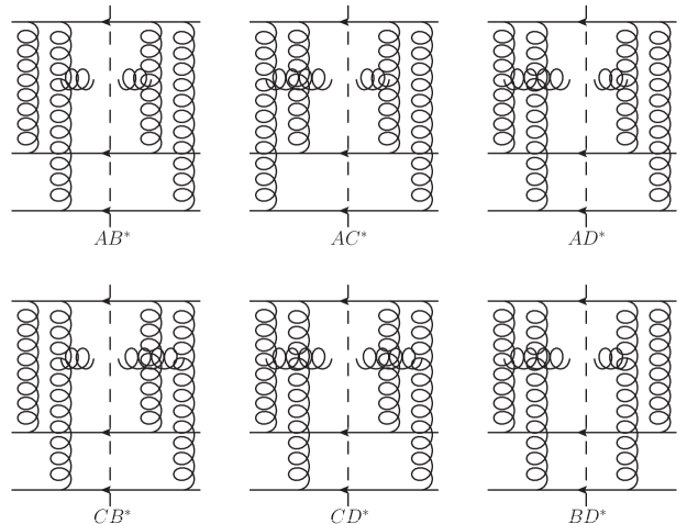
Figure 6: Interference diagrams with two R$\to$RP vertices

Obviously, $(B)\cdot(D)^{*}$ is obtained from $(A)\cdot(C)^{*}$ by the interchange of target quarks, that is, the change $\lambda\to-\lambda$. The same interchange transforms $(A)\cdot(D)^{*}$ into $(B)\cdot(C)^{*}=[(C)\cdot(B)^{*}]^{*}$, which amounts to changing $\lambda\to-\lambda$ and taking conjugate. So it is sufficient to consider 4 diagrams $(A)\cdot(B)^{*}$, $(A)\cdot(C)^{*}$, $(A)\cdot(D)^{*}$ and $(C)\cdot(D)^{*}$.

1. $(A)\cdot(B)^{*}$

The product of reggeon propagators and $R\to RP$ vertices is

$$g^{2}f^{a_{1}b_{1}c}f^{a^{\prime}_{1}b^{\prime}_{2}c}{\bf L}(p,q_{1}){\bf L}(p,q^{\prime}_{2}).$$ (56)

The colour factor is

$$C_{AB}=0.$$ (57)

The dependence on $q_{1-}$ comes from the denominators in the virtual quark propagators, which are $D_{1}$ from (48) and

$$D_{2}=(k-q^{\prime}_{1})^{2}-i0=(k-q_{1}+\lambda)^{2}-i0.$$ (58)

We get the longitudinal integral

$$I_{AB}=I(k+p-q,-k-\lambda)=0.$$ (59)

2. $(A)\cdot(C)^{*}$

The product of reggeon propagators and R$\to$RP vertices is the same as for $(A)(B)^{*}$. The colour factor is

$$C_{AC}=-\frac{N_{c}^{2}-1}{32N_{c}}.$$ (60)

The dependence on $q_{1-}$ comes from the denominators $D_{1}$ from (48) and

$$D_{2}=(k-p-q_{2}^{\prime})^{2}-i0=(k-q+q_{1}-\lambda)^{2}-i0.$$ (61)

We get the integral

$$I_{AC}=I(k+p-q,k-q-\lambda)=\frac{2\pi i}{k_{+}^{2}}\frac{1}{\lambda_{-}+\frac{q_{2\perp}^{2}}{k_{+}}-\frac{(p+q_{2})^{2}_{\perp}}{k_{+}}+i0},$$ (62)

where we neglected the term $p_{-}$ as compared to $\lambda_{-}$ in the denominator. In the limit $k_{+}\to\infty$ this develops a pole at $\lambda_{-}=0$ and will give a non-zero contribution to the inclusive cross-section.

3. $(A)\cdot(D)^{*}$

The product of reggeon propagators and $R\to RP$ vertices is the same as for the term $(A)\cdot(A)^{*}$ (46). The colour factor is

$$C_{AD}=-\frac{N_{c}^{2}-1}{16N_{c}^{3}}.$$ (63)

The denominators are $D_{1}$ from (48) and

$$D_{2}=(k-q+q_{2}^{\prime})^{2}-i0=(k-p-q_{1}+\lambda)^{2}-i0.$$ (64)

We get the integral

$$I_{AD}=I(k+p-q,-k+p-\lambda)=0.$$ (65)

4. $(C)\cdot(D)^{*}$

The product of reggeon propagators R$\to$RP vertices is the same as for $(C)\cdot(C)^{*}$ The color factor is given by (57) and equal to zero. The dependence on $q_{1-}$ comes from the denominators $D_{1}$ from (51) and $D_{2}$ from (64). We get the integral

$$I_{CD}=I(k-q,-k+p-\lambda)=0.$$ (66)

5.

As a result, interference contribution comes from diagrams

$$\Big{[}(A)\cdot(C)^{*}+(\lambda\to-\lambda)\Big{]}+c.c.$$

Supplying all the rest factors we find

$$F_{3}=-2\pi msg^{10}\frac{N_{c}^{2}-1}{N_{c}}\int\frac{d^{2}q_{1\perp}d^{2}q_{2\perp}}{(2\pi)^{4}}\frac{1}{q_{1\perp}^{4}q_{2\perp}^{4}}{\bf L}(p,q_{1}){\bf L}(p,q_{2}).$$ (67)

In the integrand there naturally appears product of Lipatov vertices. The same result follows from the BFKL-Bartels approach.

6 Interference between the R$\to$RP and R$\to$ RRP vertices

It corresponds to 4 diagrams $(E)\cdot[(A)^{*}+(B)^{*}+(C)^{*}+(D)^{*}]$ shown in in Fig. 7 plus 4 conjugated diagrams $[(A)+(B)+(C)+(D)]\cdot(E)^{*}$

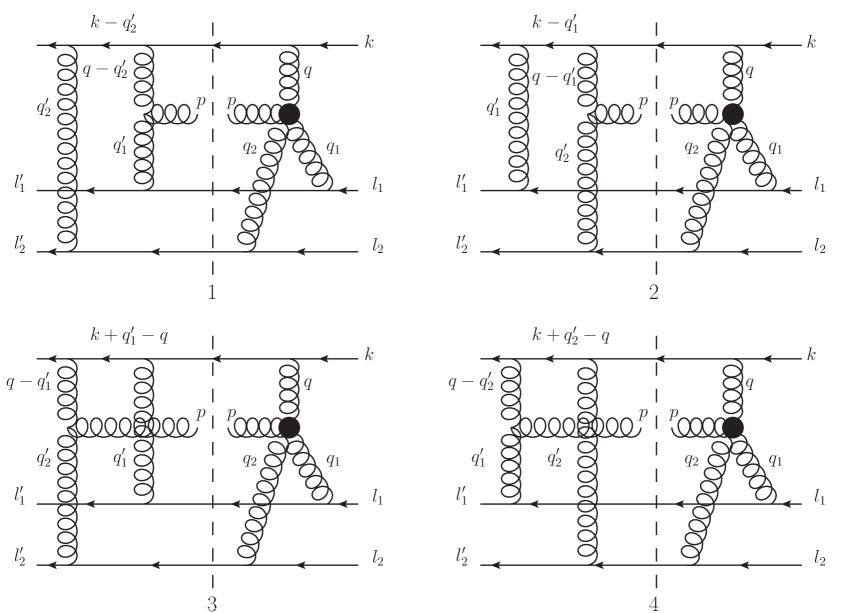
Figure 7: Interference between the R$\to$RP and R$\to$ RRP vertices

We consider only diagrams shown in Fig. 7. Obviously, $(E)\cdot(B)^{*}$ and $(E)\cdot(D)^{*}$ are obtained from $(E)\cdot(A)^{*}$ and $(E)\cdot(C)^{*}$ respectively by the interchange of the target quarks which is realized by the change $\lambda\to-\lambda$. So it is sufficient to consider only two diagrams $(E)\cdot(A)^{*}$ and $(E)\cdot(C)^{*}$.

Factors corresponding to the target quarks and the R$\to$ RRP vertex $V$ are common to all the diagrams and can be borrowed from (21), (26) and (27). The spin-momentum part of the factor corresponding to the projectile quark, also common for all the diagrams, is given by

$$-2\pi g^{3}\delta((k-q)^{2})k_{+}^{3}.$$ (68)

As mentioned, we neglect contributions coming from parts $R_{1,2}$ in $V_{1,2}$, which are absent according to  [6] and study the contributions coming from parts $W_{1,2}$ only.

1. $(W_{1})\cdot(A)^{*}$ (Fig. 7.1)

The product of reggeon propagators and $R\to RP$ and $R\to RRP$ vertices is

$$ig^{3}{f^{ab_{1}d}f^{b_{2}cd}}f^{eb^{\prime}_{1}c}\frac{q_{+}}{(q-q_{1})^{2}+i0}{\bf B}(p,q_{2},q_{1}){\bf L}(p,q^{\prime}_{1}).$$ (69)

The colour factor is

$$C_{1A}=-\frac{N_{c}^{2}-1}{32N_{c}}.$$ (70)

The dependence on $q_{1-}$ comes from the denominators in the vertex $W_{1}$:

$$D_{1}=(q-q_{1})^{2}+i0$$ (71)

and the virtual quark propagator:

$$D_{2}=(k-q_{2}^{\prime})^{2}-i0=(k+p-q+q_{1}-\lambda)^{2}-i0.$$ (72)

We get the longitudinal integral

$$I_{1A}=I(-q,k+p-q-\lambda)=0.$$ (73)

2. $(W_{1})\cdot(C)^{*}$ (Fig 7.3)

The product of reggeon propagators and $R\to RP$ and $R\to RRP$ vertices is

$$ig^{3}{f^{ab_{1}d}f^{b_{2}cd}}f^{eb^{\prime}_{2}c}\frac{q_{+}}{(q-q_{1})^{2}+i0}{\bf B}(p,q_{2},q_{1}){\bf L}(p,q^{\prime}_{2}).$$ (74)

The colour factor is

$$C_{1C}=\frac{N_{c}^{2}-1}{16N_{c}}.$$ (75)

The dependence on $q_{1-}$ comes from the denominators in the vertex $W_{1}$ and the virtual quark propagator: $D_{1}$ from (71) and

$$D_{2}=(k-p-q_{2}^{\prime})^{2}-i0=(k-q+q_{1}-\lambda)^{2}-i0.$$ (76)

We get the longitudinal integral

$$I_{1C}=I(-q,k-q-\lambda)=0.$$ (77)

3. $(W_{2})\cdot(A)^{*}$ (Fig. 7.1)

The product of reggeon propagators and $R\to RP$ and $R\to RRP$ vertices is

$$ig^{3}{f^{ab_{2}d}f^{b_{1}cd}}f^{eb^{\prime}_{1}c}\frac{q_{+}}{(q-q_{2})^{2}+i0}{\bf B}(p,q_{1},q_{2}){\bf L}(p,q^{\prime}_{1}).$$ (78)

The colour factor is

$$C_{2A}=-\frac{N_{c}^{2}-1}{16N_{c}}.$$ (79)

The longitudinal integral is

$$I_{2A}=I(p,k+p-q-\lambda)=\frac{2\pi i}{k_{+}q_{+}}\frac{1}{\lambda_{-}+\frac{(p+q_{1})^{2}_{\perp}}{q_{+}}-\frac{q_{2\perp}^{2}}{k_{+}}+i0}.$$ (80)

At both $k_{+},p_{+}\to\infty$ this gives a non-zero contribution to the inclusive cross-section.

4. $(W_{2})\cdot(C)^{*}$ (Fig. 7.3)

The product of reggeon propagators and $R\to RP$ and $R\to RRP$ vertices is

$$ig^{3}{f^{ab_{2}d}f^{b_{1}cd}}f^{eb^{\prime}_{2}c}\frac{q_{+}}{(q-q_{2})^{2}+i0}{\bf B}(p,q_{1},q_{2}){\bf L}(p,q^{\prime}_{2}).$$ (81)

The colour factor is

$$C_{2C}=\frac{N_{c}^{2}-1}{32N_{c}}.$$ (82)

The longitudinal integral is

$$I_{2C}=I(p,k-q-\lambda)=\frac{2\pi i}{k_{+}q_{+}}\frac{1}{\lambda_{-}+\frac{(p+q_{1})_{\perp}^{2}}{q_{+}}-\frac{(p+q_{2})_{\perp}^{2}}{k_{+}}+i0}.$$ (83)

At $k_{+},p_{+}\to\infty$ we get a non-zero contribution to the inclusive cross-section.

5.

The total contribution from interference terms between $(W_{1,2})$ and $(A)+(B)+(C)+(D)$ is given by

$$(W_{2})\cdot[(A)+(C)]^{*}+(\lambda\to-\lambda)+c.c.$$ (84)

Supplying all the necessary factors we find the contribution to the high-energy part

$$F_{4}=-2\pi msg^{10}\frac{N_{c}^{2}-1}{N_{c}}\int\frac{d^{2}q_{1\perp}d^{2}q_{2\perp}}{(2\pi)^{4}}\frac{1}{q_{1\perp}^{4}q_{2\perp}^{4}}{\bf B}(p,q_{2},q_{1})\Big{(}{\bf L}(p,q_{1})-2{\bf L}(p,q_{2})\Big{)}.$$ (85)

It coincides with the contribution obtained in the BFKL-Bartels approach.

7 Conclusions

The main result of this paper is that after all longitudinal integrations and with a certain restriction on the emitted gluon energy, the inclusive cross-section for gluon production can be obtained directly from the purely transverse BFKL-Bartels picture with the use of standard Lipatov-Bartels vertices, as was done in [5] on intuitive grounds. This circumstance may be very important for calculation of inclusive cross-sections in more complicated cases (such as nucleus-nucleus collisions), where avoiding longitudinal integrations may lead to substantial simplifications. To get our result it has been essential that the R$\to$RRP vertex depending on longitudinal variables and found by the direct application of the effective action approach consists of two parts $W$ and $R$. These two terms in their sum correctly describe the part of the amplitude which does not contain $\delta$-functions in the transferred ”energies” $q_{1,2-}$. The latter are supplied by the corresponding part of the contributions from the double reggeon exchange. However, alternatively, one can take the contribution from the double reggeon exchange as a whole, substituting by it the part $R$ from the R$\to$RRP effective vertex. Once this substitution has been done, the contribution coming from the remaining part $W$ together with contributions from the R$\to$RP vertices exactly coincides with what is found in the transverse space BFKL-Bartels approach and thus fully confirms its validity.

Note that in our paper  [4] this result required the principal value prescription for the integration of certain singularities in longitudinal integrals. In fact these singularities only appear in the part $R$ of the R$\to$RRP vertex. So if one drops this part altogether the principal value prescription, external with respect to the effective action formalism, becomes redundant.

We finally note once again that the found contribution is only a part of the total non-diffractive inclusive cross-section The rest comes from intermediate states with only one of the targets and requires knowledge of the R$\to$RRRP vertex. The study of the latter is in progress.

8 Acknowledgements

The authors are indebted to J.Bartels and L.N.Lipatov for helpful discussions. This work has been partially supported by the RFFI grant 09-02-01327-a (Russia).

References

[1] L.N.Lipatov, Sov. J. Nucl. Phys. 23 (1976) 338;
E.A.Kuraev, L.N.Lipatov and V.S.Fadin, Sov. Phys. JETP 45 (1977) 199;
I.I.Balitsky and L.N.Lipatov, Sov. J. Nucl. Phys. 28 (1978) 822.
[2] J.Bartels, Nucl. Phys. B175 (1980) 365.
[3] L.N.Lipatov, Phys. Rep. 286 (1997) 131.
[4] M.A.Braun, M.I.Vyazovsky,
Eur. Phys. J. C 51 (2007) 103.
[5] M.A.Braun, Eur. Phys. J. C 48 (2006) 501.
[6] M.A.Braun, L.N.Lipatov, M.Yu.Salykin and M.I.Vyazovski,
Eur. Phys. J. C 71 (2011) :1639.
[7] V.N.Gribov, Sov. Phys. JETP 29 (1969) 483.
[8] A.Capella and A.Krzywicki, Phys. Rev. D 18 (1978) 3357.