Planar approximation for the frequencies of spin transfer oscillators

Abstract

A large class of spin transfer oscillators use the free layer with a strong easy plane anisotropy, which forces its magnetization to move close to the plane. We show that in this situation the effective planar approximation provides a fast and accurate way of calculating the oscillator frequency.

I Introduction

Spin transfer devices can have regimes in which their magnetic moments perform perpetual precessional motions.slon96 ; bjz:2001 In this case they are also called spin torque oscillators (STO). Magnetic oscillations induced by direct current are intensively studied experimentally tsoi:2000 ; kiselev2003 ; rippard:2004 ; sankey:2005 ; rippard:2006 ; houssameddine:2007 ; boulle:2007 ; devolder:2007 ; houssameddine:2009 and theoretically.kent:2004 ; rezende:2005 ; bertotti:2005 ; serpico:2005:JMMM:oscillations ; serpico:2005 ; bonin:2007 ; wang2006 ; kim:2008:linewidth ; tibirkevich:2008 ; kim:2008:lineshape ; slavin:2008:IEEE In the STO regime the energy is constantly supplied to the device from the current source through the spin transfer mechanism. At the same time it is lost through the usual dissipation mechanisms, accounted for by the Gilbert damping constant. In a state of steady precession the energy gain and loss are balanced on average. In the limit of small damping one observes the following general picture of the STO operation.bertotti:2005 The magnetic moment moves close to the trajectory which it would follow in the absence of damping and spin transfer. The actual trajectory is a perturbation of the zero-damping trajectory, chosen so as to balance the small dissipation with the equally small energy gain. The main difficulty in describing the precession states is the lack of knowledge about the unperturbed trajectory which is a solution of the complicated non-linear Landau-Lifshitz-Gilbert (LLG) equation. Unless one considers a small radius precession near an equilibrium point, the analytic form of such a trajectory is usually unknown and one is forced to use numeric methods. In this paper we will consider a special class of spin transfer devices with dominating easy plane anisotropy. This anisotropy often arises from the thin disk shape of the magnetic layers found in the majority of experimental structures. Due to the dominating easy plane anisotropy the LLG equation can be approximated by an effective planar equation bazaliy:2007:APL ; bazaliy:2007:PRB ; bazaliy:2009:SPIE that is less complex and easier to treat analytically. Here we derive the planar approximation expressions for the STO oscillation periods and compare them with the numeric results obtained without approximations.

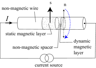
Figure 1: Spin transfer device with a fixed and free magnetic layers

II Model

We will consider the case of a spin transfer (Fig. 1) device with two magnetic layers, both described as macrospins. One of the layers has a fixed magnetic moment with a direction given by a unit vector $\bf s$. This layer acts as a spin polarizer. The other layers’s magnetization is free to move and can be described by a macrospin magnetic moment ${\bf M}(t)=M_{s}{\bf n}(t)$ where $M_{s}$ is the constant saturation magnetization and $\bf n$ is a unit vector.

The magnetic dynamics of the free layer is governed by the LLG equation with spin transfer term (see, e.g., Ref. bjz:2004, )

$${\dot{\bf n}}=\frac{\gamma}{M_{s}}\left[-\frac{\delta E}{\delta{\bf n}}\times{\bf n}\right]+u[{\bf n}\times[{\bf s}\times{\bf n}]]+\alpha[{\bf n}\times\dot{\bf n}]\ ,$$ (1)

where $E$ is the total magnetic energy of the free layer, $\gamma$ is the (positive) gyromagnetic ratio, $\alpha$ is the Gilbert damping, and the spin-transfer magnitude is given by

$$u=g(P,({\vec{n}}\cdot{\vec{s}}))\frac{\gamma(\hbar/2)}{VM_{s}}\frac{I}{e}\ ,$$ (2)

where $V$ is the free layer volume, $I$ is the electric current, and $e$ is the electron charge. The factor $I/e$ is positive when electrons flow into the free layer. Generally the spin polarization factor $g(P,({\vec{n}}\cdot{\vec{s}}))$ depends on the angle between the polarizer and the free layer and on the degree of spin polarization $P$.slon96 ; brouwer ; bauer_rmp In this paper we will employ the frequently used approximation $g=$ const. In this case $u$ is simply a rescaled current value.

We consider the free layer with an easy plane anisotropy in the $(x,y)$ plane and additional easy axis anisotropy along the $\hat{x}$ direction. External magnetic field $H$ is also applied along $\hat{x}$. The magnetic energy is given by

$$E({\bf n})=\frac{K_{p}}{2}n_{z}^{2}-\frac{K_{a}}{2}n_{x}^{2}-HM_{s}n_{x}$$ (3)

where $K_{p}$ and $K_{a}$ are the easy axis and easy plane anisotropy constants. To simplify notation we will use the rescaled energy function

$$\varepsilon({\bf n})=\frac{\gamma}{M_{s}}E=\frac{\omega_{p}}{2}n_{z}^{2}-\frac{\omega_{a}}{2}n_{x}^{2}-hn_{x}$$

where the new constants $\omega_{p}=\gamma K_{p}/M_{s}$, $\omega_{a}=\gamma K_{a}/M_{s}$, and $h=\gamma H$ have the dimensions of frequency.

The fixed layer magnetization is assumed to be pointing along the easy axis as well, ${\bf s}=+\hat{x}$.

III Effective planar description

As shown in Ref. bazaliy:2007:PRB, , when the inequalities $\omega_{p}\gg\omega_{a}$ and $\omega_{p}\gg h$ hold, vector $\bf n$ moves close to the $(x,y)$ plane and its magnetic dynamics can be described by an effective planar equation governing the behavior of its in-plane (azimuthal) angle $\phi(t)$, measured from the $x$-axis. The equation reads

$$\frac{\ddot{\phi}}{\omega_{p}}+\alpha_{eff}(\phi)\ \dot{\phi}=-\frac{d\varepsilon_{eff}}{d\phi}\ .$$ (4)

One can observe that it has a form of a Newton equation of motion for an “effective particle” with a mass $1/\omega_{p}$ moving in the external one-dimensional potential $\varepsilon_{eff}(\phi)$ with a variable friction coefficient $\alpha_{eff}(\phi)$. The effective energy and friction are found bazaliy:2007:PRB to be given by

$$\varepsilon_{eff} = -\frac{1}{2}\left(\omega_{a}+\frac{u^{2}}{\omega_{p}}\right)\cos^{2}\phi-h\cos\phi\ ,$$

$$\alpha_{eff} = \alpha+\frac{2u\cos\phi}{\omega_{p}}\ .$$ (5)

The analogy between the effective planar equation and the Newton equation for a one-dimensional particle often provides a qualitative understanding of the system’s behavior.

In the absence of spin transfer ($u=0$) one has $\alpha_{eff}=\alpha>0$, and the planar equation predicts that the solution $\phi(t)$ will approach a minimum of $\varepsilon_{eff}(\phi)$. Indeed, a particle subjected to a viscous friction force will eventually come to rest in one of the energy minima. This is guaranteed by a classical mechanics theorem, stating that the total energy

$$\varepsilon_{tot}(t)=\frac{\dot{\phi}^{2}}{2\omega_{p}}+\varepsilon_{eff}(\phi)$$ (6)

is a decreasing function of time. The theorem is based on the relationship

$$\frac{d\varepsilon_{tot}}{dt}=-\alpha_{eff}(\phi)\dot{\phi}^{2}\ ,$$ (7)

and holds for $\alpha_{eff}>0$ (case of conventional friction).

When the current is turned on, the effective friction can become negative for some values of $\phi$. In the areas of negative friction the energy of the effective particle may increase, the theorem about the decrease of $\varepsilon_{tot}(t)$ breaks down, and the particle motion does not necessarily have to stop in the local energy minimum. As a result, the effective particle can perform an oscillating motion which corresponds to the persistent precession state of the free layer.

III.1 Description of oscillation regimes

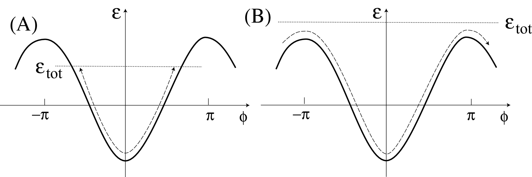
Figure 2: Oscillation states at $h>\tilde{\omega}$. The solid line gives the effective energy $\varepsilon_{eff}(\phi)$. Dashed lines with arrows show the motion of the particle in the potential profile. Horizontal dotted line gives the level of the total energy $\varepsilon_{tot}$. (A) small oscillations at $-u_{2}<u<-u_{1}$. (B) full rotations at $u<-u_{2}$.

In the case of effective energy and friction given by Eqs. 5 the effect of $u\neq 0$ was analyzed in Ref. bazaliy:2007:PRB, . We start with a review of these results. Denoting $\tilde{\omega}=\omega_{a}+u^{2}/\omega_{p}$, one finds that the effective energy has a minimum at $\phi=0$ for $h>-\tilde{\omega}$ and $\phi=\pi$ for $h<\tilde{\omega}$. Both minima are present for $|h|<\tilde{\omega}$. For small currents the effective damping is still positive for all values of $\phi$. As the current increases, $\alpha_{eff}$ first becomes negative at one of the minimum points $\phi=0$ or $\phi=\pi$ at the critical current values $u=\mp u_{1}$, where

$$u_{1}=\frac{\alpha\omega_{p}}{2}\ .$$

Negative $\alpha_{eff}$ at a point of energy minimum leads to the development of oscillations around this formerly stable equilibrium. As the current grows, the region of negative $\alpha_{eff}$ becomes larger and the oscillations amplitude increases. The evolution of oscillations at large amplitudes proceeds differently for $|h|<\tilde{\omega}$ and $|h|>\tilde{\omega}$.

In the large field case, $|h|>\tilde{\omega}$, the energy has only one minimum. For definiteness, consider the case of positive $h>\tilde{\omega}$, with the minimum of $\varepsilon_{eff}$ at $\phi=0$ and a maximum at $\phi=\pi$ (Fig. 2). The effective damping at the minimum point changes sign to negative at $u=-u_{1}$. After that the system develops small oscillations around $\phi=0$ (Fig. 2A). As the current is made even more negative, the amplitude of these oscillations grows, until at a second critical current $u=-u_{2}(h)$ it becomes so large that the effective particle reaches the point of energy maximum $\phi=\pi$. After that the particle starts to make full circles in the easy plane (Fig. 2B). The speed of the particle performing full circles becomes larger and larger as the current is decreased further below $-u_{2}$.

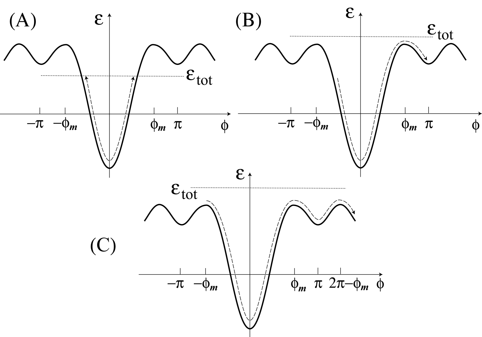
Figure 3: Oscillation states and switching at $0<h<\tilde{\omega}$. The solid line gives the effective energy $\varepsilon_{eff}(\phi)$. Dashed lines with arrows show the motion of the particle in the potential profile. Horizontal dotted line gives the level of the total energy $\varepsilon_{tot}$. (A) small oscillations at $-u_{2}<u<-u_{1}$; (B) Switching to the $\phi=\pi$ local minimum at $-u_{3}<u<-u_{2}$; (C) Full rotations at $u<-u_{3}$.

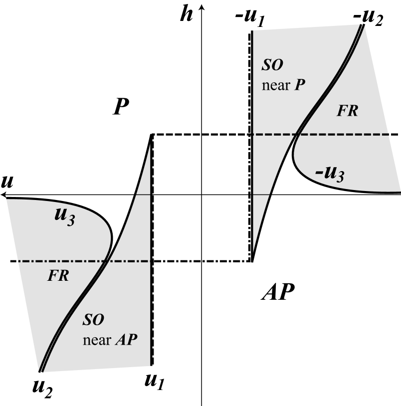
Figure 4: Switching diagram. The dashed and dash-dotted lines give the stability boundaries for the $\phi=\pi$, antiparallel (AP) and $\phi=0$, parallel (P) states respectively. These static states coexist with each other in the central rectangle of the diagram. The oscillatory regions are shown as grey areas, marked by the type of oscillation: small oscillations (SO) near P or AP points or full rotation regime (FR). Oscillations sometimes coexist with P or AP states. The diagram is symmetric in accord with the condition (8).

In the small field case, $|h|<\tilde{\omega}$, there are two minima of $\varepsilon_{eff}$ at $\phi=0$ and $\phi=\pi$ with a maximum point at the angle $\phi_{m}(h)$ between them (Fig. 3). Considering again the case of positive field $0<h<\tilde{\omega}$ one finds the following picture. The $\phi=0$ minimum is destabilized at a negative current $u=-u_{1}$ and small oscillations around this equilibrium are developed (Fig. 3A). As the current is decreased further, the amplitude of the oscillations grows until they reach the point of energy maximum at the second critical current $u=-u_{2}(h)$. For larger amplitudes the effective particle moves over the energy maximum into the basin of the $\phi=\pi$ minimum (Fig. 3B). In this basin the effective damping is positive and the particle gradually looses its total energy, ending up in the $\phi=\pi$ minimum.

There is, however, yet another transition at the third critical current $u=-u_{3}(h)$. Beyond the third threshold the particle reaches the $\phi=\phi_{m}$ maximum with a velocity that is sufficiently high to allow it to move all the way to the next energy maximum at $\phi=2\pi-\phi_{m}$, overcoming the friction force that attempts to stop it (Fig. 3C). In other words, the energy obtained in the negative damping area around $\phi=0$ is sufficient to push the particle around the full circle from $-\phi_{m}$ to $2\pi-\phi_{m}$. At $u<-u_{3}(h)$ the particle can be either in the oscillation regime with full circle rotations, or at rest in the $\phi=\pi$ energy minimum. The actual state is determined by the history of the system.

So far we have discussed small oscillations near the $\phi=0$ equilibrium and their transformation into the full rotation regime. Positive current $u>0$ can destabilize the $\phi=\pi$ equilibrium. Due to the symmetry of the problem, the critical currents $u_{i}$ of the $\phi=\pi$ equilibrium are related to those already found for $\phi=0$ as

$$u_{i}(\pi,h)=-u_{i}(0,-h)\qquad i=1,2,3$$ (8)

The switching diagrambazaliy:2007:PRB of our spin transfer system is shown in Fig. 4. It consists of the two 90-degree wedges of stability of the $\phi=0$ equilibrium (“parallel state”), and $\phi=\pi$ equilibrium (“antiparallel state”). In addition to the stability areas of the fixed points there are stability areas of the oscillating solutions (grey areas in Fig. 4). The oscillating solutions of the planar equation are in a one-to-one correspondence with the free layer precession states previously found numerically by solving the LLG equation.kiselev2003 ; xiao2005 The small oscillations regime corresponds to the case of in-plane precession of vector $\bf n$, and the full rotation regime corresponds to the out-of-plane precession.bazaliy:2007:PRB

As the current is increased deeper into the full rotation regime the deviations of $\bf n$ from the $(x,y)$ easy plane plane grow, and the planar approximation becomes inapplicable. The orbits of persistent precession evolve bertotti:2005 ; xiao2005 ; slavin:2008:IEEE into small circles around the maximum of the magnetic energy (3) far away from the easy plane. Eventually this point is stabilized by spin transfer.bjz:2001 ; bjz:2004

III.2 Small damping approximation

Consider first the planar equation (4) at $u=0$. In the limit of $\alpha\to 0$ the friction term can be viewed as a perturbation on top of the frictionless motion. When friction is completely absent, the total energy is exactly conserved

$$\varepsilon_{tot}(t)=\varepsilon_{tot}(0)$$ (9)

For small friction $\varepsilon_{tot}$ is conserved approximately, i.e., its relative change during one period of oscillations around the potential minimum is small. On a time scale of several periods one can approximately use equation (9). For longer time intervals one has to take into account that $\varepsilon_{tot}(t)$ is a slowly changing function of time.

In the case of $u\neq 0$ the same picture holds as long as the absolute value of $\alpha_{eff}$ is small. The only difference is that now the total energy can either decrease or grow during one period of oscillations. Here we want to note that the smallness of $|\alpha_{eff}|$ is already guaranteed by the smallness of $\alpha$ in the following sense. As discussed above, the oscillating regimes of spin transfer systems appear when the effective damping becomes negative. At the onset of the oscillation regime the Gilbert damping term and the spin transfer term in the expression for $\alpha_{eff}$ are of the same order. That means that $|\alpha_{eff}|$ and $\alpha$ have the same order of magnitude, unless the current is increased far above the threshold.

The slow time change of $\varepsilon_{tot}$ can be calculated using the following procedure. We use Eq. (7) to find the energy change during one period of oscillations

$$\Delta=-\int_{0}^{T}\alpha_{eff}\dot{\phi}^{2}dt\ .$$

Applying the approximate energy conservation during the period one can express the particle velocity as

$$\dot{\phi}\approx\pm\sqrt{2\omega_{p}(\varepsilon_{tot}-\varepsilon_{eff}(\phi))}=f(\phi,\varepsilon_{tot})$$ (10)

where $\varepsilon_{tot}$ is assumed to be constant, for example taken as the value of the total energy at the beginning of the period. The plus or minus sign in front of the expression is chosen according to the direction of particle motion. The electric current parameter $u$ enters $\alpha_{eff}$ as a linear correction, and $\varepsilon_{eff}$ as a quadratic correction. It will be shown in Sec. III.4 that the correction to the effective energy can be dropped in our approximation and $\varepsilon_{eff}$ can be substituted by $\varepsilon(\phi)=-(1/2)\omega_{a}\cos^{2}\phi-h\cos\phi$ in Eq. (10), i.e., one can use $\omega_{a}$ instead of $\tilde{\omega}$.

Using approximation (10) one finds both $\Delta$ and the oscillation period $T$ as

$$\Delta \approx -\oint\alpha_{eff}(\phi)f(\phi)\ d\phi\ ,$$ (11)

$$T = \int_{0}^{T}dt=\oint\frac{d\phi}{\dot{\phi}}\approx\oint\frac{d\phi}{f(\phi)}\ .$$

In these formulae the integrals over $\phi$ are taken along the closed trajectory corresponding to one period of oscillations in the absence of damping and spin transfer. The value of $\varepsilon_{tot}$ determines both the integration limits, and the integrand. Consequently, equations (11) give both $\Delta$ and $T$ as the functions of $\varepsilon_{tot}$. The slow time evolution of the total energy is described by an approximate equation

$$\frac{d\varepsilon_{tot}}{dt}\approx\frac{\Delta(\varepsilon_{tot})}{T(\varepsilon_{tot})}$$ (12)

In the regime of persistent oscillations the total energy is constant, which implies $\Delta(\varepsilon_{tot})=0$. In Ref. bazaliy:2007:PRB, this condition was used to find the critical currents $u_{i}$ by the following argument. The critical trajectories corresponding to each $u_{i}$ were already described in Sec. III.1. On those trajectories the value of $\varepsilon_{tot}$ is given by the value of $\varepsilon_{eff}$ at the turning points where $\dot{\phi}=0$. Now the integral (11) can be calculated as a function of $u$, and the equation $\Delta(u)=0$ gives a current threshold.

III.3 Oscillation periods

Here we use (12) to calculate the period of oscillations with arbitrary amplitude. Our goal is to find the function $T(u)$. The equation $d\varepsilon_{tot}/dt=0$ or $\Delta=0$ holds for persistent oscillation regimes at any current, not just for the critical current values. At a given $u$ this equation determines the value of $\varepsilon_{tot}$ and the endpoints of the integration contour in the first equation of the system (11). Knowing them, we can calculate $T$ from the second equation in (11) and find the function $T(u)$.

We will do the calculations for $u<0$. According to the symmetry of the switching diagram (Fig. 4) the $u>0$ results can be easily obtained from those for $u<0$.

III.3.1 Case of $h>\omega_{a}$

Here one observes small oscillations for $-u_{2}<u<-u_{1}$ and full rotations for $u<-u_{2}$.

In the small oscillations regime the particle moves between the points of maximum deviation $\pm\phi_{a}$ (Fig. 2A). The total energy is given by $\varepsilon_{tot}=\varepsilon(\phi_{a})=(1/2)\omega_{a}\cos^{2}\phi_{a}-h\cos\phi_{a}$, and the expression (10) specializes to

$$\dot{\phi} \approx \pm\Omega\sqrt{R(\phi)}\ ,$$

$$R(\phi,\phi_{a},h) = \cos^{2}\phi-\cos^{2}\phi_{a}+\frac{2h}{\omega_{a}}(\cos\phi-\cos\phi_{a})\ ,$$

$$\Omega = \sqrt{\omega_{a}\omega_{p}}\ .$$

Condition $\Delta=0$ together with (11) gives

$$\int_{-\phi_{a}}^{\phi_{a}}\left(\alpha+\frac{2u\cos\phi}{\omega_{p}}\right)\Omega\sqrt{R(\phi)}\ d\phi=0$$

or

$$\alpha K_{1}(\phi_{a})+\frac{2u}{\omega_{p}}K_{2}(\phi_{a})=0$$

with

$$K_{1}(\phi_{a})=\int_{-\phi_{a}}^{\phi_{a}}\sqrt{R(\phi)}\ d\phi\ ,$$

$$K_{2}(\phi_{a})=\int_{-\phi_{a}}^{\phi_{a}}\cos\phi\sqrt{R(\phi)}\ d\phi\ .$$

We can now express the current as a function of the oscillation amplitude $\phi_{a}$

$$u(\phi_{a})=-\frac{\alpha\omega_{p}}{2}\frac{K_{1}(\phi_{a})}{K_{2}(\phi_{a})}\ .$$ (13)

The second equation of (11) gives the oscillation period, also expressing it as a function of $\phi_{a}$

$$T(\phi_{a})=2\int_{-\phi_{a}}^{\phi_{a}}\frac{d\phi}{\Omega\sqrt{R(\phi)}}=\frac{2K_{3}(\phi_{a})}{\Omega}\ .$$ (14)

Using equations (13) and (14) one can make a parametric plot $T(u)$ by varying $\phi_{a}$ from zero to $\pi$. The integrals $K_{i}$ can be expressed through special functions or, in practice, calculated by a computer algebra system.

The boundary between the small oscillations and the full rotations is found at the current value

$$-u_{2}(h)=u(\pi)=-\frac{\alpha\omega_{p}}{2}\frac{K_{1}(\pi,h)}{K_{2}(\pi,h)}\quad(h>\omega_{a})\ ,$$ (15)

where we have explicitly indicated the dependence of the integrals on $h$. Note that this formula corrects formula (8) from Ref. bazaliy:2007:PRB, which is valid only for the values of $h$ slightly above $\omega_{a}$, i.e., for $h-\omega_{a}\ll\omega_{a}$.

Below the $-u_{2}$ threshold the oscillations happen with a full rotation of the angle $\phi$. There are no endpoints here (Fig. 2B) and we will parameterize the trajectory by the excess energy $\Delta\varepsilon=\varepsilon_{tot}-\varepsilon(\pi)>0$. Equation (10) specializes to

$$\dot{\phi}=\Omega\sqrt{R(\phi,\pi,h)+\frac{2\omega_{p}\Delta\varepsilon}{\Omega}}=\Omega\sqrt{R(\phi,\pi,h)+\delta}$$

where we have introduced $\delta=2\omega_{p}\Delta\varepsilon/\Omega$. Repeating the steps that led to equations (13) and (14) we get an analogous pair of equations for the full rotation regime

$$u(\delta) = -\frac{\alpha\omega_{p}}{2}\frac{L_{1}(\delta)}{L_{2}(\delta)}$$ (16)

$$T(\delta) = \frac{L_{3}(\delta)}{\Omega}$$ (17)

where the integrals $L_{i}$ are expressed through $\tilde{R}=R(\phi,\pi,h)$ as

$$L_{1}(\delta)=\int_{-\pi}^{\pi}\sqrt{\tilde{R}(\phi)+\delta}\ d\phi$$

$$L_{2}(\delta)=\int_{-\pi}^{\pi}\cos\phi\sqrt{\tilde{R}(\phi)+\delta}\ d\phi$$

$$L_{3}(\delta)=\int_{-\pi}^{\pi}\frac{d\phi}{\sqrt{\tilde{R}(\phi)+\delta}}$$

Using equations (16) and (17) one can make a parametric plot $T(u)$ by varying $\delta$ from zero up.

III.3.2 Case of $|h|<\omega_{a}$

For small oscillations ($-u_{2}<u<-u_{1}$), the calculations turn out to be identical with those performed in the previous section. Expressions (13) and (14) can be used to make a parametric plot $T(u)$. The only difference is that now the oscillation amplitude $\phi_{a}$ changes form zero to the angle $\phi_{m}$ of the energy maximum.

The critical current $u_{2}(h)$ is found by setting $\phi_{a}=\phi_{m}$. The position of the energy maximum is found from the equation $d\varepsilon/d\phi=0$ which gives

$$\cos\phi_{m}=-\frac{h}{\omega_{a}}\ .$$

At the same time the expression for $R$ can be rewritten as

$$R=\left(\cos\phi+\frac{h}{\omega_{a}}\right)^{2}-\left(\cos\phi_{a}+\frac{h}{\omega_{a}}\right)^{2}$$

As a result, for $\phi_{a}=\phi_{m}$ one is able to write an explicit formula for the square root

$$\sqrt{R(\phi,\phi_{m},h)}=|\cos\phi+h/\omega_{a}|\ .$$ (18)

The integrals $K_{1,2}$ can be then taken and one gets the expression for the critical currentbazaliy:2007:PRB

$$u_{2}=\alpha\omega_{p}\frac{\sin\phi_{m}+(h/\omega_{a})\phi_{m}}{\phi_{m}+(h/\omega_{a})\sin\phi_{m}},\quad(|h|<\omega_{a})\ .$$ (19)

The third critical current $u=-u_{3}(h)$ corresponds to the trajectory shown in Fig. 3C. The angle changes from $-\phi_{m}$ to $2\pi-\phi_{m}$, and the total energy is equal to $\varepsilon(2\pi-\phi_{m})$ because at the critical current the particle starts at $-\phi_{m}$ with zero velocity, makes a full rotation, and reaches $2\pi-\phi_{m}$ with zero velocity. Since $\varepsilon(2\pi-\phi_{m})=\varepsilon(\phi_{m})$, we find that the condition $\Delta=0$ specializes to

$$\int_{-\phi_{m}}^{2\pi-\phi_{a}}\left(\alpha+\frac{2u\cos\phi}{\omega_{p}}\right)\sqrt{R(\phi,\phi_{m},h)}\ d\phi=0$$

(the integrand is the same as in the case of small oscillations but the integration limits are different). Using equation (18) we then findbazaliy:2007:PRB

$$u_{3}=\alpha\omega_{p}\frac{\sin\phi_{m}+(h/\omega_{a})(\phi_{m}-\pi/2)}{(\phi_{m}-\pi/2)+(h/\omega_{a})\sin\phi_{m}},\quad(|h|<\omega_{a})\ .$$ (20)

For the currents exceeding the third threshold, $u<-u_{3}$, there are no turning points and, similar to the case of large fields, we parameterize the trajectory by the scaled energy excess over the maximum: $\delta=2\omega_{p}(\varepsilon(\phi)-\varepsilon(\phi_{m}))/\Omega>0$. The resulting parametric expressions for the current and period turn out to be identical to Eqs. (16) and (17), except that the meaning of $\tilde{R}$ changes to $\tilde{R}=R(\phi,\phi_{m},h)=(\cos\phi+h/\omega_{a})^{2}$ in the definitions of the integrals $L_{1,2,3}$.

Overall, equation pairs (13, 14) and (16, 17) give the planar approximation formulae for the periods of all spin transfer oscillations possible in our system. For small oscillations regime with current just above the first threshold the results (14) and (17) give the frequencies converging to $\sqrt{(\omega_{a}+h)\omega_{p}}$, i.e., to the Kittel’s formula with a substitution $\omega_{p}+h\to\omega_{p}$ in accord with our approximation $h\ll\omega_{p}$. For other current values we will present the results of the theory as graphs (Figs. 5 and 6) for the periods $T(u,h)$ rather than for the frequencies since oscillations periods are more directly interpreted in terms of effective particle analogy.

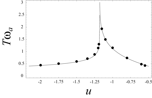
Figure 5: Large field case. Comparison between the no-approximation numeric results (dots) and planar approximation expressions (lines) for the oscillations periods. Here $\omega_{p}=100\ \omega_{a}$, $h=1.4\ \omega_{a}$, $\alpha=0.01$. The oscillation period diverges at $u=-u_{2}$

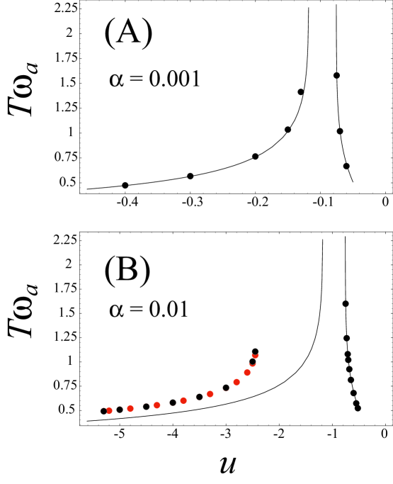
Figure 6: (Color online) Small field case. Comparison between the no-approximation numeric results (dots) and planar approximation expressions (line) for the oscillations periods for $\omega_{p}=100\ \omega_{a}$, $h=0.5\ \omega_{a}$. The oscillation period diverges at $u=-u_{2}$ and $u=-u_{3}$ with no oscillations between the two thresholds. Top panel (A) gives results for $\alpha=0.001$, where the agreement is very good. The bottom panel (B) shows a comparison for $\alpha=0.01$. Planar approximation works well for small precession, but the full rotations regime requires currents which are too large for the small friction approximation (16, 17) to be accurate. The exact solution of the planar equation (red (grey) dots) is still in very good agreement with the numeric solution of the LLG equation (black dots).

III.4 Condition of small damping

The validity of the small damping approximation for Eq. (4) requires

$$\Delta\ll\varepsilon_{tot}\ .$$ (21)

We can make a rough estimate by noting that in the regime of $h\sim\omega_{a}$ the value of $R$ is of the order of one. The current magnitude is assumed to be such that the spin transfer term in $\alpha_{eff}$ is of the same order as bare $\alpha$. Then the formula (11) gives

$$\Delta\sim\alpha\Omega\ .$$

As for the total energy, we assume that it has the same order of magnitude as the magnetic energy

$$\varepsilon_{tot}\sim\varepsilon\sim\omega_{a}\ .$$

With the above estimates the small damping condition (21) transforms into

$$\alpha\ll\sqrt{\frac{\omega_{a}}{\omega_{p}}}\ .$$ (22)

This is a well known condition of small Gilbert damping in planar systems.bazaliy:2007:APL ; weinan-e

We can now show that the current-dependent term in $\tilde{\omega}=\omega_{a}+u^{2}/\omega_{p}$ is a small correction to $\omega_{a}$ whenever the conditions (22) holds. Indeed, for currents of the same order as the critical current we have $u\sim\alpha\omega_{p}$, so

$$\frac{u^{2}}{\omega_{p}}\sim\alpha^{2}\omega_{p}\ll\omega_{a}\ .$$

This estimate justifies our statement in Sec. III.2.

IV Comparison with the no-approximation numeric results

Oscillation periods can be found numerically by solving the LLG equation without approximations. In practice this means rewriting the vector equation (1) in polar angles $\theta$ and $\phi$ of the unit vector ${\bf n}=\{n_{x},n_{y},n_{z}\}=\{\sin\theta\cos\phi,\sin\theta\sin\phi,\cos\theta\}$. One obtains a system

$$\dot{\phi} = \frac{F_{\phi}+\alpha F_{\theta}}{(1+\alpha^{2})\sin\theta}\ ,$$

$$\dot{\theta} = \frac{F_{\theta}-\alpha F_{\phi}}{1+\alpha^{2}}\ ,$$ (23)

with

$$F_{\phi} = -\sin\theta\cos\theta(\omega_{p}+\omega_{a}\cos^{2}\phi)-h\cos\theta\cos\phi$$

$$-u\sin\phi\ ,$$

$$F_{\theta} = -\omega_{a}\sin\theta\sin\phi\cos\phi-h\sin\phi+u\cos\theta\cos\phi\ .$$

The system is solved numerically with Mathematica. When an oscillating solution exists, the motion of $\bf n$ approaches the same precession cycle regardless of the initial conditions, as long as they are its basin of attraction. The period of the precession motion is measured after the stationary regime is achieved.

Fig. 5 compares the numeric LLG results with the planar approximation formula for the high field case, $h>\omega_{a}$. One observes a very good correspondence. Near the critical current $u=-u_{2}$ the periods of oscillations become infinite and their frequencies drop to zero.bertotti:2005 This is easy to understand from the effective particle analogy: at the critical current the particle travels between the two maxima of the energy profile that have the same height with the particle energy being equal to the potential energy at the maximum point. As it usually happens in such cases, the motion near the maximum is infinitely slow and the period is infinite.

In the low field case, $0<h<\omega_{a}$, the comparison of numeric and approximate results is shown in Fig. 6. In the top panel (Fig. 6A) the Gilbert damping is set to $\alpha=0.001$, and the condition $|\alpha_{eff}|\ll\sqrt{\omega_{a}/\omega_{p}}$ is well satisfied for all current magnitudes on the graph. The correspondence between the numeric LLG results and the small damping approximation to the planar equation is very good. As expected, the oscillations period diverges at $u=-u_{2}$ and $u=-u_{3}$, with no oscillations between the two thresholds.

Fig. 6B shows results for $\alpha=0.01$. We observe good correspondence between the LLG numeric results and our theory for the small oscillations, but the full rotations regime shows appreciable differences which become very large near the critical current. Their origin is the breakdown of the small damping approximation: for $\alpha=0.01$ the currents in the full rotation regime are so large that the strong inequality $|\alpha_{eff}|\ll\sqrt{\omega_{a}/\omega_{p}}$ is not well satisfied. To prove that the small damping approximation is the source of the discrepancy we have solved the planar equation (4) numerically. The results (red (gray) dots in Fig. 6B) correspond very well to those obtained directly from LLG (black dots in Fig. 6B).

It is also instructive to compare the cases of large and small fields with the same value of Gilbert damping $\alpha=0.01$ (Fig. 5 and Fig. 6B). One can see that the validity region of the small damping approximation extends at least to $u\approx-2$ in the case of large field. At the same time in the case of small fields this approximation is visibly violated for $u\approx-2$. The relative fragility of the small damping approximation in the full rotation regime in small fields can be traced to the presence of two energy maxima, $\phi=\pm\phi_{m}$, instead of just one maximum, $\phi=\pi$, in the large fields. The situation calls for more work on the approximate solutions of the effective planar equation (4) with variable damping.

V Conclusions

We have shown that the planar approximation bazaliy:2007:APL ; bazaliy:2007:PRB gives good results for the frequencies of spin transfer oscillators with dominating easy plane anisotropy. Analytic expressions for the oscillation periods were derived in the limit of small Gilbert damping. The mechanical analogy, associated with the effective planar equation, provides a qualitative understanding of different precession regimes and naturally explains the singular behavior of the precession frequency near the transition between in-plane and out-of-plane precessions.

An important advantage of the planar approximation is the fact that the problem of finding the unperturbed trajectory is drastically simplified. All one-dimensional trajectories are straight lines completely characterized by their endpoints. This property should help to develop theories of the large-angle precession regimes of planar spin torque oscillators in the presence of temperature fluctuations or other noise sources.

VI Acknowledgements

This work was supported by the NSF grant DMR-0847159.

References

- (1) J. Slonczewski, J. Magn. Magn. Mater. 159, L1 (1996).
- (2) Ya. B. Bazaliy, B.A.Jones, and Shou-Cheng Zhang, J. Appl. Phys. 89, 6793 (2001).
- (3) M. Tsoi, A. G. M. Jansen, J. Bass, W.-C. Chiang, V. Tsoi, and P. Wyder, Nature 406, 46 (2000).
- (4) S. I. Kiselev, J. C. Sankey, I. N. Krivorotov, N. C. Emley, R. J. Schoelkopf, R. A. Buhrman, and D. C. Ralph, Nature, 425, 380 (2003).
- (5) W. H. Rippard, M. R. Pufall, S. Kaka, S. E. Russek, and T. J. Silva, Phys. Rev. Lett. 92, 027201 (2004).
- (6) J. C. Sankey, I. N. Krivorotov, S. I. Kiselev, P. M. Braganca, N. C. Emley, R. A. Buhrman, and D. C. Ralph, Phys. Rev. B 72, 224427 (2005).
- (7) W. H. Rippard, M. R. Pufall, and S. E. Russek, Phys. Rev. B 74, 224409 (2006).
- (8) D. Houssameddine, U. Ebels, B. Dela t, B. Rodmacq, I. Firastrau, F. Ponthenier, M. Brunet, C. Thirion, J.-P. Michel, L. Prejbeanu-Buda, M.-C. Cyrille, O. Redon, B. Dieny, Nature Materials 6, 447 (2007).
- (9) O. Boulle, V. Cros, J. Grollier, L. G. Pereira, C. Deranlot, F. Petroff, G. Faini, J. Barnas, and A. Fert, Nature Physics 3, 492 (2007) .
- (10) T. Devolder, A. Meftah, K. Ito, J. A. Katine, P. Crozat, and C. Chappert, J. Appl. Phys., 101, 063916 (2007).
- (11) D. Houssameddine, U. Ebels, B. Dieny, K. Garello, J.-P. Michel, B. Delaet, B. Viala, M.-C. Cyrille, J. A. Katine, and D. Mauri, Phys. Rev. Lett. 102, 257202 (2009).
- (12) A. D. Kent, B. Ozyilmaz, and E. del Barco, Appl. Phys. Lett. 84, 3897 (2004).
- (13) S. M. Rezende, F. M. de Aguiar, and A. Azevedo, Phys. Rev. Lett. 94, 037202 (2005).
- (14) G. Bertotti, C. Serpico, I. D. Mayergoyz, A. Magni, M. d’Aquino, and R. Bonin, Phys. Rev. Lett. 94, 127206 (2005).
- (15) C. Serpico, M. d’Aquino, G. Bertotti, and I. D. Mayergoyz, J. Magn. Magn. Mat. 290-291, 502 (2005).
- (16) C. Serpico, J. Magn. Magn. Mat. 290-291, 48 (2005).
- (17) R. Bonin, C. Serpico, G. Bertotti, I. D. Mayergoyz and M. d’Aquino, Eur. Phys. J. B 59, 435 (2007).
- (18) X. Wang, G. E. W. Bauer, and A. Hoffmann, Phys. Rev. B, 73, 054436 (2006).
- (19) J.-V. Kim, V. Tiberkevich, and A. N. Slavin, Phys. Rev. Lett. 100, 017207 (2008).
- (20) V. S. Tiberkevich, A. N. Slavin, and J.-V. Kim, Phys. Rev. B 78, 092401 (2008).
- (21) J.-V. Kim, Q. Mistral, C. Chappert, V. S. Tiberkevich, and A. N. Slavin, Phys. Rev. Lett. 100, 167201 (2008).
- (22) A. Slavin and V. Tiberkevich, IEEE Trans. Magn. 44, 1916 (2008).
- (23) Ya. B. Bazaliy, Appl. Phys. Lett. 91, 262510, (2007).
- (24) Ya. B. Bazaliy, Phys. Rev. B 76, 140402(R), (2007).
- (25) Ya. B. Bazaliy, Proceedings of SPIE Conference, Spintronics II, 7398, 73980P-1 (2009).
- (26) Ya. B. Bazaliy, B. A. Jones, and Shou-Cheng Zhang, Phys. Rev. B, 69, 094421 (2004).
- (27) X. Waintal, E. B. Myers, P. W. Brouwer, and D. C. Ralph, Phys. Rev. B, 62, 12317 (2000).
- (28) Y. Tserkovnyak, A. Brataas, G. E. W. Bauer, and B. I. Halperin, Rev. Mod. Phys. 77, 1375 (2005).
- (29) J. Xiao, A. Zangwill, and M. D. Stiles, Phys. Rev. B, 72, 014446 (2005).
- (30) C. J. Garica-Cervera, Weinan E, J. Appl. Phys., 90, 370 (2001).