Planar approximation for spin transfer systems
with application to tilted polarizer devices

Abstract

Planar spin-transfer devices with dominating easy-plane anisotropy can be described by an effective one-dimensional equation for the in-plane angle. Such a description provides an intuitive qualitative understanding of the magnetic dynamics. We give a detailed derivation of the effective planar equation and use it to describe magnetic switching in devices with tilted polarizer.

I Introduction

The spin-transfer effect is a non-equilibrium interaction that arises when a current of electrons flows through a non-collinear magnetic texture berger ; slon96 ; bjz1997 . Spin transfer torque can lead to current induced magnetic switching in multilayer devices or domain wall motion in devices with continuous change of magnetization. Both phenomena serve as an underlying mechanism for a number of suggested memory and logic applications.

Magnetic dynamics in spin-transfer devices can be described by the Landau-Lifshitz-Gilbert (LLG) equation. Analytic solutions of LLG can be easily found in the simplest case of easy axis magnetic anisotropy. However, when the form of anisotropy energy becomes more complicated the investigations of the stability of static equilibria become much more involved. A study of the precession cycles is even more complicated and often makes it necessary to resort to numeric simulations. Due to the complexity of the LLG equation it is always interesting to consider cases where some simplifying approximations can be made.

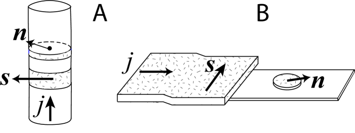
In many devices the easy plane anisotropy energy is much larger than the other anisotropy energies, and the system is in the planar spintronic device regime bauer-planar-review (Fig. 1). The limit of dominating easy plane energy is characterized by a simplification of the dynamic equations weinan-e , which comes not from the high symmetry of the problem, but from the existence of a small parameter: the ratio of the energy modulation within the plane to the easy plane energy. The deviation of the magnetization from the plane becomes small, making the motion effectively one dimensional. As a result, an effective description in terms of just one azimuthal angle becomes possible.

Figure 1: Planar spin-transfer devices. Hashed parts of the devices are ferromagnetic, clear parts are made from a non-magnetic metal.

Our publications boj:2008 ; bazaliy:2007:APL ; bazaliy:2007:PRB ; bazaliy:2009:SPIE introduced the planar approximation in the presence of spin-transfer torques and listed a number of results highlighting the practical use of the method. In this paper we give a detailed derivation the effective planar equation for a macrospin free layer in the presence of spin transfer torques (Sec. III). We then show in Sec. IV how this equation can be applied to a system with the tilted polarizer and obtain a qualitative picture of the device dynamics.

II Magnetic dynamics of the free layer

We consider a conventional spin-transfer device consisting of a a magnetic polarizer (fixed layer) and a small magnet (free layer) with electric current flowing from one to another (Fig. 1). The free layer is influenced by the spin transfer torque, while the polarizer is too large to feel it. It is assumed that due to the large exchange stiffness the free layers can be described by a macrospin model. Its magnetic dynamics is described by the Landau-Lifshitz-Gilbert equation with the spin transfer torque term.

The state of the free layer is characterized by just one vector, its total magnetic moment ${\bf M}=M{\bf n}$ which has a constant absolute value $M$ and a direction given by a unit vector ${\bf n}(t)$. The LLG equation slon96 ; bjz2004 reads:

$${\dot{\bf n}}=\left[-\frac{\delta\varepsilon}{\delta{\bf n}}\times{\bf n}\right]+u({\bf n})[{\bf n}\times[{\bf s}\times{\bf n}]]+\alpha[{\bf n}\times\dot{\bf n}]\ .$$ (1)

Here the re-scaled energy $\varepsilon=(\gamma/M)E$ has the dimensions of frequency and is expressed through the total magnetic energy $E({\bf n})$ of the free layer; $\gamma$ is the gyromagnetic ratio, and $\alpha$ is the Gilbert damping constant. The second term on the right is the spin transfer torque. Unit vector ${\bf s}$ points along the direction of the polarizer moment, and the spin transfer strength $u({\bf n})$ is proportional to the electric current $I$ bjz2004 . In general, spin transfer strength is a function of the angle between the polarizer and the free layer $u({\bf n})=g[({\bf n}\cdot{\bf s})]\ I$. The spin current efficiency factor $g[({\bf n}\cdot{\bf s})]$ is a material and device specific function.

In polar angles $(\theta,\phi)$ equation (1) reads

$$\dot{\theta}+\alpha\dot{\phi}\sin\theta = -\frac{1}{\sin\theta}\frac{\partial\varepsilon}{\partial\phi}+u({\bf n})({\bf s}\cdot{{\bf e}_{\theta}})\ ,$$

$$\dot{\phi}\sin\theta-\alpha\dot{\theta} = \frac{\partial\varepsilon}{\partial\theta}+u({\bf n})({\bf s}\cdot{\bf e}_{\phi})\ ,$$ (2)

where the unit tangent vectors ${\bf e}_{\theta}$ and ${\bf e}_{\phi}$ are defined in the Appendix A.

We assume that the easy plane is defined by $\theta=\pi/2$, and the rescaled magnetic energy has the form

$$\varepsilon=\frac{\omega_{p}}{2}\cos^{2}\theta+\varepsilon_{r}(\theta,\phi)\ .$$

The first term represents the easy plane anisotropy, with the planar frequency $\omega_{p}$ related to the easy plane constant $K_{p}$ as $\omega_{p}=\gamma K_{p}/M$. The remainder $\varepsilon_{r}$ is the “residual” energy. The planar limit is characterized by $\omega_{p}\to\infty$. Large easy plane constant forces the energy minima to be very close to the easy plane and the low energy solutions of LLG to have the property $\theta(t)=\pi/2+\delta\theta$ with $\delta\theta\to 0$. Equations (2) can then be expanded in small parameters

$$\frac{|\varepsilon_{r}|}{\omega_{p}}\ll 1\quad{\rm and}\quad\frac{|u({\bf n})|}{\omega_{p}}\ll 1\ .$$

By truncating this expansion one obtains the effective planar approximation.

III Derivation of the effective planar equation

Explicitly separating the large easy plane terms, we rewrite equation (2) as

$$\dot{\theta}+\alpha\dot{\phi}\sin\theta = f_{\theta}+u_{\theta}$$

$$\dot{\phi}\sin\theta-\alpha\dot{\theta} = -\omega_{p}\cos\theta\sin\theta+f_{\phi}+u_{\phi}$$

where the residual anisotropy is responsible for the terms

$$f_{\theta}(\theta,\phi) = -\frac{1}{\sin\theta}\frac{\partial\varepsilon_{r}}{\partial\phi}\ ,$$

$$f_{\phi}(\theta,\phi) = \frac{\partial\varepsilon_{r}}{\partial\theta}\ ,$$ (3)

and the spin transfer torque produces the terms

$$u_{\theta}(\theta,\phi) = u({\bf n})({\bf s}\cdot{\bf e}_{\theta})\ ,$$

$$u_{\phi}(\theta,\phi) = u({\bf n})({\bf s}\cdot{\bf e}_{\phi})\ .$$ (4)

We also introduce a notation $F_{\theta,\phi}=f_{\theta,\phi}+u_{\theta,\phi}$, and re-write the LLG system as

$$\dot{\theta} = \frac{F_{\theta}-\alpha(-\omega_{p}\cos\theta\sin\theta+F_{\phi})}{1+\alpha^{2}}$$

$$\dot{\phi} = \frac{-\omega_{p}\cos\theta\sin\theta+F_{\phi}+\alpha F_{\theta}}{(1+\alpha^{2})\sin\theta}$$

Next, we make the approximations. In the $\omega_{p}\to\infty$ limit the solution is expected to have a property $\theta(t)=\pi/2+\delta\theta(t)$ with $\delta\theta\to 0$. Expanding all quantities on the r.h.s. of (LABEL:eq:dotthetadotphi) in small $\delta\theta$ up to the first order we get

$$\delta{\dot{\theta}} = \frac{F^{0}_{\theta}+F^{1}_{\theta}\delta\theta-\alpha(\omega_{p}\delta\theta+F^{0}_{\phi}+F^{1}_{\phi}\delta\theta)}{1+\alpha^{2}}\ ,$$ (6)

$$\dot{\phi} = \frac{\omega_{p}\delta\theta+F^{0}_{\phi}+F^{1}_{\phi}\delta\theta+\alpha(F^{0}_{\theta}+F^{1}_{\theta}\delta\theta)}{1+\alpha^{2}}\ ,$$ (7)

where we have used the notation

$$F^{0} = F\left(\frac{\pi}{2},\phi\right)\ ,$$

$$F^{1} = \frac{\partial F}{\partial\theta}\left(\frac{\pi}{2},\phi\right)\ .$$

In the approximation (6,7) equations are linear with respect to the unknown function $\theta(t)$, but still fully non-linear with respect to $\phi(t)$.

Eq. (7) can be viewed as an equation on $\delta\theta$ which gives

$$\delta\theta=\frac{(1+\alpha^{2})\dot{\phi}-F^{0}_{\phi}-\alpha F^{0}_{\theta}}{\omega_{p}+F^{1}_{\phi}+\alpha F^{1}_{\theta}}=q(\phi,\dot{\phi})$$ (8)

so that the out-of-plane deviation becomes a “slave” of the in-plane motion.weinan-e The presence of the large $\omega_{p}$ in the denominator ensures the smallness of $\delta\theta$. Substituting the resulting expression $\delta\theta=q(\phi,\dot{\phi})$ back into equation (6) one obtains a second order differential equation for a single unknown function $\phi(t)$

$$\frac{\partial q}{\partial\dot{\phi}}\ \ddot{\phi}+\frac{\partial q}{\partial\phi}\ \dot{\phi}=\frac{F^{0}_{\theta}-\alpha F^{0}_{\phi}}{1+\alpha^{2}}+\left(\frac{F^{1}_{\theta}-\alpha\omega_{p}-\alpha F^{1}_{\phi}}{1+\alpha^{2}}\right)q\ .$$

By denoting $\Omega(\phi)=\omega_{p}+F^{1}_{\phi}+\alpha F^{1}_{\theta}$ and simplifying the terms we get

$$\frac{1+\alpha^{2}}{\Omega}\ddot{\phi} + \left(\alpha+\frac{\partial q}{\partial\phi}-(1+\alpha^{2})\frac{F^{1}_{\theta}}{\Omega}\right)\dot{\phi}=$$ (9)

$$= F^{0}_{\theta}-\frac{F^{1}_{\theta}(F^{0}_{\phi}+\alpha F^{0}_{\theta})}{\Omega}$$

In this form the equation is still too complicated to be useful but since it was obtained from the approximations (6,7) we are allowed to drop the terms that are smaller or equal to the already neglected ones. Those were the $F^{\prime\prime}\delta\theta^{2}$ terms in the expansion of $F$, and the third order terms $\omega_{p}\delta\theta^{3}$ in the easy plane energy expansion. While formally the latter are of higher order in the $\delta\theta$ expansion, the large coefficient $\omega_{p}$ can causes them to have the same order of magnitude.

To compare the orders of magnitude of the terms consistently, we need to know the order of magnitude of $\delta\theta$. At the present stage we know that $\delta\theta$ is small but its exact order of magnitude is not known because we do not have an estimate for the $\dot{\phi}$ term in the numerator of Eq. (8).

III.1 Simple residual energy in the absence of spin torque

To estimate $\delta\theta$, let us first consider the problem in the absence of spin transfer ($F=f$),weinan-e assuming a simple form of residual energy $\varepsilon_{r}=\varepsilon_{r}(\phi)$. In this case we find $f^{0}_{\phi}=f^{1}_{\phi}=f^{1}_{\theta}=0$ and get

$$q(\phi,\dot{\phi})=\frac{(1+\alpha^{2})\dot{\phi}-\alpha f^{0}_{\theta}}{\omega_{p}}\ .$$ (10)

Equation (9) takes a form

$$\frac{1+\alpha^{2}}{\omega_{p}}\ddot{\phi}+\alpha\left(1-\frac{1}{\omega_{p}}\frac{\partial f^{0}_{\theta}}{\partial\phi}\right)\dot{\phi}=f^{0}_{\theta}\ .$$

Assuming that the residual energy $\varepsilon_{r}(\phi)$ does not have any special points of fast change we can estimate $F^{0}_{\theta}\sim\varepsilon\ll\omega_{p}$. Then

$$1-\frac{1}{\omega_{p}}\frac{\partial f^{0}_{\theta}}{\partial\phi}\approx 1$$

and we can approximate the equation by

$$\frac{1+\alpha^{2}}{\omega_{p}}\ddot{\phi}+\alpha\dot{\phi}=f^{0}_{\theta}=-\frac{\partial\varepsilon_{r}}{\partial\phi}\ .$$

The equation above has the form of the Newton’s equation for a particle of mass $(1+\alpha^{2})/\omega_{p}$ moving in a one-dimensional potential $\varepsilon_{r}(\phi)$, subject to a viscous friction force with a friction coefficient $\alpha$. Our goal is to estimate the value of $\dot{\phi}$, i.e., the speed of the “effective particle”.

The particle’s characteristic speed depends on the total energy and on the relative strength of the friction forces. We will assume that the energy is of the order of $\varepsilon_{r}$ (this is the mathematical equivalent of our original assumption about the low-energy dynamics of the moment). Furthermore, in the present paper we will concentrate on the case of $\alpha\to 0$ that corresponds to an almost frictionless motion of the particle. Then one can use the approximate energy conservation and write $(1/2\omega_{p})\dot{\phi}^{2}=\varepsilon_{r}$ for the maximum speed. This gives

$$\dot{\phi}\sim\sqrt{\varepsilon_{r}\omega_{p}}$$

Using similar arguments one can estimate the maximum acceleration as

$$\ddot{\phi}\sim\varepsilon_{r}\omega_{p}$$

Note that the viscous friction can be approximately neglected when $\alpha\dot{\phi}\ll F^{0}_{\theta}\sim\varepsilon_{r}$, i.e., the Gilbert damping constant $\alpha$ has to be not just small compared to unity but satisfy a more stringent inequality

$$\alpha\ll\sqrt{\frac{\varepsilon_{r}}{\omega_{p}}}\ll 1\ .$$ (11)

We see now that $\dot{\phi}$ is the largest term in the denominator of (10) and as a result obtain an estimate

$$\delta\theta\sim\sqrt{\frac{\varepsilon_{r}}{\omega_{p}}}\ .$$ (12)

III.2 Arbitrary residual energy in the absence of spin torque

Let us return to the approximation (6,7) with the general form of the residual energy $\varepsilon_{r}=\varepsilon_{r}(\theta,\phi)$ and zero current, $u=0$, $F=f$. It is now possible to use the a posteriori estimate (12) for $\delta\theta$ to consider the orders of magnitude of the terms on the right hand sides of the equations. We start the discussion from the “slave” equation (7). Here

$$\omega_{p}\delta\theta \sim \sqrt{\varepsilon_{r}\omega_{p}}$$

$$f^{0} \sim \varepsilon_{r}$$

$$f^{1}\delta\theta \sim \varepsilon_{r}\sqrt{\frac{\varepsilon_{r}}{\omega_{p}}}$$

$$\alpha f^{0} \ll \varepsilon_{r}\sqrt{\frac{\varepsilon_{r}}{\omega_{p}}}$$

$$\alpha f^{1}\delta\theta \ll \varepsilon_{r}\frac{\varepsilon_{r}}{\omega_{p}}$$

As we see, the orders of magnitude of the terms form a series

$$\ldots\quad\varepsilon_{r}\frac{\varepsilon_{r}}{\omega_{p}},\quad\varepsilon_{r}\sqrt{\frac{\varepsilon_{r}}{\omega_{p}}},\quad\varepsilon_{r},\quad\sqrt{\varepsilon_{r}\omega_{p}}\quad\ldots$$ (13)

with the general term given by $\varepsilon_{r}(\varepsilon_{r}/\omega_{p})^{n/2}$.

The terms neglected in transition from system (LABEL:eq:dotthetadotphi) to (7) were

$$\omega_{p}\delta\theta^{3} \sim \varepsilon_{r}\sqrt{\frac{\varepsilon_{r}}{\omega_{p}}}\ ,$$

$$\frac{\partial^{2}f}{\partial\theta^{2}}\delta\theta^{2} \sim \varepsilon_{r}\frac{\varepsilon_{r}}{\omega_{p}}\ .$$

This means that in (7) one should only keep the terms of the order $\varepsilon_{r}$ and higher. Lower order terms would be comparable to some of the discarded terms. Using this argument we discard $f^{1}\delta\theta$, $\alpha f^{0}$ and $\alpha f^{1}\delta\theta$. The $1/(1+\alpha^{2})$ factor in (7) can be expanded using Eq. (11)

$$\frac{1}{1+\alpha^{2}}=1+\delta,\quad\delta\sim\alpha^{2}\ll\frac{\varepsilon_{r}}{\omega_{p}}\ .$$

This inequality shows that $1/(1+\alpha^{2})$ can can be approximated by unity in Eq. (7) without changing the accuracy. After those simplifications equation (8) takes the form

$$q(\phi,\dot{\phi})=\frac{\dot{\phi}-f^{0}_{\phi}}{\omega_{p}}\ ,$$

As for the equation (6), the terms discarded in going from (LABEL:eq:dotthetadotphi) to (6) were

$$\alpha\omega_{p}\delta\theta^{3} \ll \varepsilon_{r}\frac{\varepsilon_{r}}{\omega_{p}}$$

$$\frac{\partial^{2}f}{\partial\theta^{2}}\delta\theta^{2} \sim \varepsilon_{r}\frac{\varepsilon_{r}}{\omega_{p}}$$

and therefore we have to keep the terms of the orders $\varepsilon_{r}\sqrt{\varepsilon_{r}/\omega_{p}}$ and higher. Thus the $f^{1}\delta\theta$ and $\alpha f^{0}$ terms should be kept in (6) but the $\alpha F^{1}\delta\theta$ terms should be discarded. One can also conclude that it is safe to replace the $1/(1+\alpha^{2})$ factor by unity. Equation (6) is now replaced by

$$\delta{\dot{\theta}}=f^{0}_{\theta}+f^{1}_{\theta}\delta\theta-\alpha(\omega_{p}\delta\theta+f^{0}_{\phi})\ ,$$

where one should use

$$f^{1}_{\theta}\delta\theta=f^{1}_{\theta}\frac{\dot{\phi}-f^{0}_{\phi}}{\omega_{p}}\approx\frac{f^{1}_{\theta}\dot{\phi}}{\omega_{p}}\ ,$$

since the term $f^{1}_{\theta}f^{0}_{\phi}/\omega_{p}\sim\varepsilon_{r}^{2}/\omega_{p}$ is of the same order as the already discarded terms.

Re-deriving Eq. (9) in this approximation one gets

$$\frac{\ddot{\phi}}{\omega_{p}}+\left(\alpha-\frac{1}{\omega_{p}}\left[\frac{\partial f^{0}_{\phi}}{\partial\phi}+f^{1}_{\theta}\right]\right)\dot{\phi}=f^{0}_{\theta}=-\frac{\partial\varepsilon_{r}(\pi/2,\phi)}{\partial\phi}$$

This is the equation for the effective particle as discussed in the previous section, except that the viscous friction coefficient seems to acquire a correction. While the correction is of the order $\varepsilon_{r}/\omega_{p}$, it is added to a small number $\alpha$ and thus can potentially have a significant effect of changing the sign of the dissipation term. However, one finds

$$\frac{\partial f^{0}_{\phi}}{\partial\phi}+f^{1}_{\theta}=\frac{\partial}{\partial\phi}\frac{\partial\varepsilon_{r}}{\partial\theta}+\frac{\partial}{\partial\theta}\left(-\frac{\partial\varepsilon_{r}}{\partial\phi}\right)=0\ ,$$ (14)

so the correction actually vanishes. We come back to the effective equation

$$\frac{\ddot{\phi}}{\omega_{p}}+\alpha\dot{\phi}=-\frac{\partial\varepsilon_{r}(\pi/2,\phi)}{\partial\phi}\ ,$$

which corresponds to the most natural generalization of the equation derived in the previous section for a special form of the residual energy $\varepsilon_{r}=\varepsilon_{r}(\phi)$. The positive effective friction coefficient ensures that the effective particle always stops in the point of energy minimum, as expected for a closed system with dissipation described by the LLG equation without spin torques.

III.3 Effective equation in the presence of spin torque

Finally, we proceed to the derivation of the effective equation in the presence of the spin torque. Consider approximations (6,7) with $\varepsilon_{r}=\varepsilon_{r}(\theta,\phi)$ and $u\neq 0$.

The order of magnitude of the extra terms produced by the current will depend on the value of $u$. One condition that certainly has to be satisfied is the smallness of the spin torque compared to the anisotropy torques produced by the easy plane contribution. The latter are responsible for the terms of the order $\sqrt{\varepsilon_{r}\omega_{p}}$ in Eqs (6,7). Thus it seems that $u$ should not exceed $\varepsilon_{r}$, which is the largest term before $\sqrt{\varepsilon_{r}\omega_{p}}$ in the series (13). Such a conclusion is correct for a general situation. We will, however, see below that in some special cases the current can be increased up to $u\sim\sqrt{\varepsilon_{r}\omega_{p}}$ without violating the dominance of the easy plane anisotropy torque.

To include those cases we assume $u\lesssim\sqrt{\varepsilon_{r}\omega_{p}}$ and revisit Eqs. (6,7) discarding the terms smaller than $\varepsilon_{r}\sqrt{\varepsilon_{r}/\omega_{p}}$ in Eq. (6), and smaller than $\varepsilon_{r}$ in Eq. (7).

Eq. (7) which acquires the form

$$\dot{\phi}=(\omega_{p}+u_{\phi}^{1})\delta\theta+f^{0}_{\phi}+u^{0}_{\phi}\ .$$

(as in the previous section, one can prove that the factor $1/(1+\alpha^{2})$ can be approximated by unity without loss of accuracy). By solving for $\delta\theta$ and expanding the denominator up to the same accuracy we find the form of the slave condition (8)

$$\delta\theta=\left(1-\frac{u^{1}_{\phi}}{\omega_{p}}\right)\frac{\dot{\phi}}{\omega_{p}}-\frac{f^{0}_{\phi}+u^{0}_{\phi}}{\omega_{p}}+\frac{u^{1}_{\phi}u^{0}_{\phi}}{\omega_{p}^{2}}$$ (15)

Differentiating both sides one gets

$$\delta\dot{\theta} = \left(1-\frac{u^{1}_{\phi}}{\omega_{p}}\right)\frac{\ddot{\phi}}{\omega_{p}}-\frac{\partial u^{1}_{\phi}}{\partial\phi}\frac{\dot{\phi}^{2}}{\omega_{p}^{2}}-$$ (16)

$$-\left(\frac{\partial f^{0}_{\phi}}{\partial\phi}+\frac{\partial u^{0}_{\phi}}{\partial\phi}-\frac{1}{\omega_{p}}\frac{\partial\big{[}u^{1}_{\phi}u^{0}_{\phi}\big{]}}{\partial\phi}\right)\frac{\dot{\phi}}{\omega_{p}}$$

Returning to Eq. (6) we find that with the declared accuracy it can be rewritten as

$$\delta\dot{\theta}=f^{0}_{\theta}+u^{0}_{\theta}-\alpha u^{0}_{\phi}+\left(f^{1}_{\theta}+u^{1}_{\theta}-\alpha\omega_{p}\right)\delta\theta\ .$$

Substituting $\delta\theta$ from (15) and discarding any terms that are smaller than $\varepsilon_{r}\sqrt{\varepsilon_{r}/\omega_{p}}$, we get

$$\delta\dot{\theta} = f^{0}_{\theta}+u^{0}_{\theta}-\left(\alpha-\frac{f^{1}_{\theta}+u^{1}_{\theta}}{\omega_{p}}+\frac{u^{1}_{\theta}u^{1}_{\phi}}{\omega_{p}^{2}}\right)\dot{\phi}-$$

$$-\frac{f^{1}_{\theta}u^{0}_{\phi}+u^{1}_{\theta}f^{0}_{\phi}+u^{1}_{\theta}u^{0}_{\phi}}{\omega_{p}}+\frac{u^{1}_{\theta}u^{1}_{\phi}u^{0}_{\phi}}{\omega_{p}^{2}}$$

The last step is to use Eq. (16) to express $\delta\dot{\theta}$ on the left hand side. This gives the form of the effective equation (9) without the terms below our accuracy

$$\left(1-\frac{u^{1}_{\phi}}{\omega_{p}}\right)\frac{\ddot{\phi}}{\omega_{p}}+$$

$$+\left(\alpha-\frac{1}{\omega_{p}}\left[\frac{\partial f^{0}_{\phi}}{\partial\phi}+f^{1}_{\theta}+\frac{\partial u^{0}_{\phi}}{\partial\phi}+u^{1}_{\theta}\right]-\right.$$

$$\left.\quad\quad\ -\frac{1}{\omega_{p}^{2}}\left[\frac{\partial\big{[}u^{1}_{\phi}u^{0}_{\phi}\big{]}}{\partial\phi}-u^{1}_{\theta}u^{1}_{\phi}\right]\right)\dot{\phi}-\frac{\partial u^{1}_{\phi}}{\partial\phi}\frac{\dot{\phi}^{2}}{\omega_{p}^{2}}=$$

$$=f^{0}_{\theta}+u^{0}_{\theta}-\frac{f^{1}_{\theta}u^{0}_{\phi}+u^{1}_{\theta}f^{0}_{\phi}+u^{1}_{\theta}u^{0}_{\phi}}{\omega_{p}}+\frac{u^{1}_{\theta}u^{1}_{\phi}u^{0}_{\phi}}{\omega_{p}^{2}}\ ,$$

where identity (14) can be used to simplify the bracketed expression on the second line.

We now cast the effective planar equation in its final form

$$m\ddot{\phi}+\alpha_{eff}\dot{\phi}-\frac{(u^{1}_{\phi})^{\prime}}{\omega_{p}^{2}}\dot{\phi}^{2}=-(\varepsilon_{eff})^{\prime}\ .$$ (17)

Here primes denote differentiation with respect to $\phi$, and the parameters are given by

$$m = \frac{1}{\omega_{p}}\left(1-\frac{u^{1}_{\phi}}{\omega_{p}}\right)\ ,$$

$$\alpha_{eff} = \alpha-\frac{(u^{0}_{\phi})^{\prime}+u^{1}_{\theta}}{\omega_{p}}+\frac{\big{(}u^{1}_{\phi}u^{0}_{\phi}\big{)}^{\prime}+u^{1}_{\phi}u^{1}_{\theta}}{\omega_{p}^{2}}\ ,$$ (18)

$$\varepsilon_{eff} = \varepsilon_{r}\left(\frac{\pi}{2},\phi\right)+U\ ,$$

$$-U^{\prime} = u^{0}_{\theta}-\frac{f^{1}_{\theta}u^{0}_{\phi}+u^{1}_{\theta}f^{0}_{\phi}+u^{1}_{\theta}u^{0}_{\phi}}{\omega_{p}}+\frac{u^{1}_{\theta}u^{1}_{\phi}u^{0}_{\phi}}{\omega_{p}^{2}}\ .$$

Equations (17) and (18) constitute the first main result of this paper.

In the presence of the current, $u\neq 0$, the right hand side of (17) contains additional “effective forces” added to the $-{\varepsilon_{r}}^{\prime}$ term. Since all functions depend on just one variable $\phi$, these forces can be always represented as the derivatives of an additional energy $U$ according to the definition (18).

One of the forces, namely the $u^{0}_{\theta}$ term, requires a special discussion. When $u\sim\sqrt{\varepsilon_{r}\omega_{p}}$ this term becomes larger than ${\varepsilon_{r}}^{\prime}$ on the right hand side of Eq. (17), and the estimates for $\dot{\phi}$ and $\ddot{\phi}$ made in Sec. III.1 become invalid. As it was discussed above, this means that in a general case with non-zero $u^{0}_{\theta}$ the effective equations (17, 18) can be only used for currents $u\lesssim\varepsilon_{r}$. However, if $u^{0}_{\theta}$ is identically equal to zero, while the other spin torque terms in $U$ and $\alpha_{eff}$ remain non-zero, one can apply Eqs. (17, 18) for currents up to $u\sim\sqrt{\varepsilon_{r}\omega_{p}}$.

Corrections to the friction coefficient are explicitly dependent on the current magnitude. In the presence of spin torque the sign of the friction coefficient may change bazaliy:2007:APL ; bazaliy:2007:PRB ; boj:2008 ; bazaliy:2009:SPIE , reflecting the possible influx of the energy from the current source into the system.

Below we investigate the application of the effective planar equation to the device with a “tilted polarizer” geometry.

IV Tilted polarizer device

In tilted polarizer devices vector $\bf s$ is pointed at an angle $\theta_{s}$ to the axis $z$ and constitutes an angle $\pi/2-\theta_{s}$ with the easy plane. We will assume that $\bf s$ is in the $(x,z)$ plane, i.e., $\phi_{s}=0$.

To calculate $u_{\theta}$ and $u_{\phi}$ from Eq. (4) one needs to know the function $u({\bf n})$. In many cases slon96 ; slonczewski:2002 it has a form

$$u({\bf n})=\frac{g_{0}I}{1+g_{1}({\bf n}\cdot{\bf s})}$$

We will consider the case of small $g_{1}\ll 1$ and approximate

$$u({\bf n})=g_{0}I(1-g_{1}({\bf n}\cdot{\bf s}))$$ (19)

Using the expressions in Appendix A, we find

$$u_{\theta} = g_{0}I\left[1-g_{1}(\sin\theta_{s}\sin\theta\cos\phi+\cos\theta_{s}\cos\theta)\right]$$

$$\times(\sin\theta_{s}\cos\theta\cos\phi-\cos\theta_{s}\sin\theta)\ ,$$

$$u_{\phi} = -g_{0}I\left[1-g_{1}(\sin\theta_{s}\sin\theta\cos\phi+\cos\theta_{s}\cos\theta)\right]$$

$$\times\sin\theta_{s}\sin\phi\ .$$

Therefore

$$u^{0}_{\theta} = -g_{0}I\left[1-g_{1}\sin\theta_{s}\cos\phi\right]\cos\theta_{s}\ ,$$

$$u^{0}_{\phi} = -g_{0}I\left[1-g_{1}\sin\theta_{s}\cos\phi\right]\sin\theta_{s}\sin\phi.$$ (20)

and

$$u^{1}_{\theta} = -g_{0}I[\sin\theta_{s}\cos\phi+g_{1}(\sin^{2}\theta_{s}\cos^{2}\phi-\cos^{2}\theta_{s})]\ ,$$

$$u^{1}_{\phi} = -g_{0}Ig_{1}\sin\theta_{s}\cos\theta_{s}\sin\phi\ .$$ (21)

IV.1 In-plane polarizer

In the case of in-plane polarizer with $\theta_{s}=\pi/2$ further simplifications happen:

$$u^{0}_{\theta} = 0$$

$$u^{0}_{\phi} = -(1-g_{1}\cos\phi)\sin\phi$$

$$u^{1}_{\theta} = -(1-g_{1}\cos\phi)\cos\phi$$

$$u^{1}_{\phi} = 0$$

As we see, the in-plane polarizer is one of the special cases with $u^{0}_{\theta}=0$, discussed at the end of Sec. III.3. Consequently, the effective equation can be used up to the currents $u\sim g_{0}I\sim\sqrt{\varepsilon_{r}\omega_{p}}$. The coefficients (18) acquire the form

$$m = \frac{1}{\omega_{p}}\ ,$$

$$\alpha_{eff} = \alpha+\frac{g_{0}I\big{[}2\cos\phi-g_{1}(3\cos^{2}\phi-1)\big{]}}{\omega_{p}}\ ,$$ (22)

$$-U^{\prime} = -\frac{g_{0}I(1-g_{1}\cos\phi)}{\omega_{p}}\times$$

$$\times \left[g_{0}I(1-g_{1}\cos\phi)\sin\phi\cos\phi\ -\right.$$

$$\qquad\qquad\left.-(f^{1}_{\theta}\sin\phi+f^{0}_{\phi}\cos\phi)\right]\ .$$

Importantly, the $\dot{\phi}^{2}$ term in Eq. (17) vanishes identically.

In Refs. bazaliy:2007:APL, ; bazaliy:2007:PRB, the in-plane polarizer was considered in the case of $g_{1}=0$ and residual energy

$$\varepsilon_{r}=-\frac{\omega_{a}}{2}\sin^{2}\theta\cos^{2}\phi-h\sin\theta\cos\phi\ ,$$ (24)

describing a device with small easy axis anisotropy $\omega_{a}\ll\omega_{p}$ in an external magnetic field $h$, both pointed along the $x$ axis. In this case one finds $f^{1}_{\theta}=f^{0}_{\phi}=0$ and expressions (IV.1) reproduce the results obtained in Refs. bazaliy:2007:APL, and bazaliy:2007:PRB, .

IV.2 General case of a tilted polarizer

When the polarizer magnetization $\bf s$ points at an arbitrary angle $\theta_{s}$ the term $u^{0}_{\theta}$ is nonzero and we have to limit the current magnitudes to $g_{0}I\lesssim\varepsilon_{r}$ to maintain the validity of Eq. (17). With smaller currents more terms can be discarded from the effective equation without changing its accuracy. Parameter expressions (18) reduce to

$$m = \frac{1}{\omega_{p}}\ ,$$

$$\alpha_{eff} = \alpha-\frac{(u^{0}_{\phi})^{\prime}+u^{1}_{\theta}}{\omega_{p}}\ ,$$ (25)

$$-U^{\prime} = u^{0}_{\theta}\ .$$

Moreover, for $g_{0}I\lesssim\varepsilon_{r}$ the nonlinear term with $\dot{\phi}^{2}$ becomes small enough to be dropped from Eq. (17).

The effective planar equation now reads

$$\frac{\ddot{\phi}}{\omega_{p}}+\alpha_{eff}\dot{\phi}=-\frac{\partial\varepsilon_{eff}}{\partial\phi}\ ,$$ (26)

where the effective damping and the effective energy can be expressed through the polarizer tilting angle $\theta_{s}$ using Eqs. (20), (21), and (25)

$$\alpha_{eff} = \alpha+\frac{g_{0}I}{\omega_{p}}(2\sin\theta_{s}\cos\phi-g_{1}[3\sin^{2}\theta_{s}\cos^{2}\phi-1])\ ,$$

$$\varepsilon_{eff} = \varepsilon_{r}(\frac{\pi}{2},\phi)+g_{0}I(\cos\theta_{s}\cdot\phi-g_{1}\sin\theta_{s}\cos\theta_{s}\sin\phi)\ .$$

IV.3 Switching diagram of the tilted polarizer device

Let us now discuss the consequences of the modification of $\alpha\to\alpha_{eff}$ and $\varepsilon_{r}\to\varepsilon_{eff}$ in the presence of spin torque. The advantage of the effective planar approximation is the possibility of using the analogy with the particle motion which enables one to use mechanical intuition to qualitatively predict the behavior of the solutions of Eq. (26), and thus understand the dynamics of the spin-transfer device.

We will assume the standard nanopillar device described by the residual energy (24). In the special case of an in-plane polarizer this problem was discussed in our earlier publications.bazaliy:2007:APL ; bazaliy:2007:PRB ; bazaliy:2009:SPIE Modifications of the effective damping transform the particle motion qualitatively when $\alpha_{eff}(\phi)$ changes sign. Modifications of $\varepsilon_{eff}(\phi)$ become qualitatively important when equilibrium points appear or disappear as the energy profile is deformed.

Figure 2: Effective energy profile in the case of a tilted polarizer.

Our goal here is to generalize the results of Refs. bazaliy:2007:APL, ; bazaliy:2007:PRB, ; bazaliy:2009:SPIE, to the case of a non-zero polarizer tilt and show that the effective planar approach allows one to understand the qualitative picture of the motion without doing the detailed calculations. The case of a tilted polarizer was considered in recent publications Zhou:2009 ; He:2010 using conventional methods. The switching diagrams were calculated assuming that $\bf s$ is tilted straight up from the easy axis direction. This corresponds to our assumption of $\phi_{s}=0$. It was also assumed that there is no magnetic field, $h=0$. We adopt the assumptions of Refs. Zhou:2009, and He:2010, to illustrate the application of the formalism developed in this paper.

In the case of a general tilt angle $\theta_{s}$ the terms containing a small factor $g_{1}$ give negligible corrections in the expressions (LABEL:eq:effective_parameters_u_order_E_through_thetaS) for $\alpha_{eff}$ and $\varepsilon_{eff}$. They can only become important when $\theta_{s}$ approaches zero or $\pi/2$ and the main terms vanish. We will assume that $\bf s$ is not to close to either the in-plane or the perpendicular directions and an inequality $\cos\theta_{s},\sin\theta_{s}\gg g_{1}$ holds. Then we can use the simplified form of Eqs. (LABEL:eq:effective_parameters_u_order_E_through_thetaS)

$$\alpha_{eff} = \alpha+\frac{2g_{0}I\sin\theta_{s}}{\omega_{p}}\cos\phi\ ,$$

$$\varepsilon_{eff} = \varepsilon_{r}(\frac{\pi}{2},\phi)+g_{0}I\cos\theta_{s}\cdot\phi\ .$$ (28)

Finding the critical currents in the narrow bands of angles $\theta_{s}\approx 0$ or $\approx\pi/2$ where the $g_{1}$ terms are important would require a more careful consideration.

Figure 3: Effective particle performing a 360^∘ motion, starting from the energy maximum $M_{1}$ and reaching an equivalent maximum $M_{3}$. The red (gray) interval denotes the region of $\alpha_{eff}<0$.

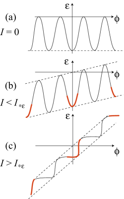
The profile of the energy $\varepsilon_{eff}(\phi)$ is shown in Fig. 2. The spin torque produces the tilted washboard potential in which the effective particle moves. The washboard tilt reflects the fact that spin torques can change the magnetic energy of the system by using work performed by the current source. The energy minima are shifted from their zero current positions at $\phi=0$ (parallel, or $P$ state) and $\phi=\pi$, (antiparallel, or $AP$ state) to the new positions $\phi_{0}(I)$ that are given by the equation

$$\sin 2\phi_{0}=\frac{2g_{0}I\cos\theta_{s}}{\omega_{a}}\ .$$

One can check that the energy minima located at the angles $\phi_{0min}+\pi n$ are still separated by the energy maxima located at at $\phi_{0max}=\pi/2-\phi_{0min}+\pi n$ (Fig. 2b). To be concise will still call the $\phi_{0min}$ minimum the $P$-point, and the $\phi_{0min}+\pi$ minimum the $AP$ point.

As the current grows, the washboard tilts more and more, until the extrema or $\varepsilon_{eff}(\phi)$ disappear altogether (Fig. 2c). A short calculations shows that this occurs at a critical current

$$I_{*\varepsilon}=\frac{\omega_{a}}{2g_{0}\cos\theta_{s}}\ .$$ (29)

For $I>I_{*\varepsilon}$ the effective particle slides down the slope of the potential energy profile regardless of the sign and magnitude of $\alpha_{eff}$. This corresponds to $\bf n$ performing full 360^∘ rotations in the azimuthal angle $\phi$. In the spin transfer literature such a regime is called the out-of-plane (OPP) precession.

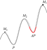
Importantly, the OPP precession can exist even at $I<I_{*\varepsilon}$. When the particle moves down the washboard, the drop of its potential energy during one spatial period may be large enough to overcome the friction energy loss (Fig. 3). Therefore there must be a second critical current $I_{OPP}<I_{*\varepsilon}$, such that the OPP precession happens for $I>I_{OPP}$. In the interval $I_{OPP}<I<I_{*\varepsilon}$ the stationary equilibrium of the particle at the energy minimum coexists with the state of OPP precession. The functional form of $I_{OPP}(\theta_{s})$ depends on the energy profile and the friction coefficient. Our goal here is not to find the expression for it, but to see how far can we proceed in qualitative understanding of the device dynamics without doing the actual calculations.

Figure 4: (a) Effective particle performing small oscillations (IPP precession) near the minimum corresponding to the AP state that lies within he red (gray) interval of $\alpha_{eff}<0$. (b) With growing current the amplitude of the oscillations increases and the particle reaches the $M_{2}$ maximum point. Above this threshold the IPP precession is unstable.

The effective damping $\alpha_{eff}$ changes its sign in the vicinity of the angles $\phi_{+n}=2\pi(n+1/2)$ for $I>0$ and $\phi_{-n}=2\pi n$ for $I<0$ when the current magnitude exceeds the threshold

$$I_{*\alpha}=\frac{\alpha\omega_{p}}{2g_{0}\sin\theta_{s}}\ .$$ (30)

The regions of $\alpha_{eff}<0$ are shown in Figs. 2,3 by red (gray) thicker line. On the intervals of negative friction the system acquires energy instead of loosing it. This makes it easier for the particle to achieve the state of the OPP precession. The actual calculation of the $I_{OPP}$ threshold must take into account the energy gain due to the tilt of the potential and the presence of negative friction intervals. Both features mathematically represent the ability of the spin torques to transfer energy from the current source to the system.

Another important effect of negative $\alpha_{eff}$ is the local destabilization of the energy minima. If the minimum point $\phi_{0}(I)$ lies within the interval of $\alpha_{eff}<0$, it becomes unstable and small oscillations around it are developed. Fig. 4a shows such oscillations near the AP minimum which, according to Eq. (28), is destabilized for $I>0$. These oscillations correspond to the precession of $\bf n$ around the equilibrium point and are called an in-plane (IPP) precession in the spin transfer literature.

The amplitude of the oscillations is determined by the balance of energy influx and dissipation on the intervals of negative and positive friction.bazaliy:2007:APL ; bazaliy:2007:PRB ; bazaliy:2009:SPIE As the current is increased, the amplitude grows and eventually becomes so large that the particle reaches the crest of the potential (Fig. 4b) and falls down into the neighboring valley. This process leads to the destruction of the IPP state. The latter therefore exists between the two threshold currents. For the $AP$ equilibrium these are the $I_{AP}$ threshold, where the $AP$ point becomes unstable, and the $I_{IPP}$ threshold, where the precession amplitude becomes too large to be contained in the $AP$ valley.

The critical current of minimum point destabilization is determined from the equation $\alpha_{eff}(\phi_{0}(I))=0$ which can be rewritten as

$$I_{AP}\cos[\phi_{0}(I_{AP})]=I_{*\alpha}\ ,$$

$$I_{P}\cos[\phi_{0}(I_{P})]=-I_{*\alpha}\ ,$$ (31)

for $P$ and $AP$ minima. The equations show that the threshold currents satisfy $|I|>I_{*\alpha}$ in both cases. This result can be naturally understood as follows. The friction first becomes negative at the $\phi=0$ or $\phi=\pi$ points at $I=\pm I_{*\alpha}$. But the $P$ and $AP$ minima are shifted from the $0,\pi$ points to the $\phi_{0}(I)$ points. In order to destabilize them the negative friction interval has to grow large enough to cover the actual minima positions.

The critical current $I_{IPP}$ depends on the shape of the potential in the entire interval traveled by the particle in Fig. 4b. Its actual calculation is not the goal of our qualitative approach. We can make two general statements about $I_{IPP}$. First, the destabilization of the precession state certainly happens at a current that is larger than the one required for the destabilization of the corresponding energy minimum. For example, $I_{IPP}>I_{AP}$.

Figure 5: Critical lines of the $P/AP$ equilibrium states and the IPP precession state on the $(I,\theta_{s})$ switching diagrams. Each line is marked by the name of the state which gets destabilized on it. The name is put on the side of the line where the state is stable. Inset: an impossible arrangement of the $AP$ and $IPP$ lines.

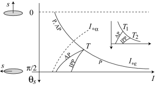
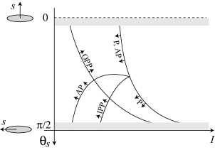
To set the stage for the second observation, we proceed to the discussion of the switching diagram. In our case the experimental parameters are the current $I$ and the tilting angle $\theta_{s}$. Various critical currents are represented as lines on the $(I,\theta_{s})$ plane and divide it into domains with different sets of stable states. The currents $I_{*\varepsilon}$, $I_{*\alpha}$, $I_{AP}$, and $I_{APP}$ are sketched as functions of the angle $\theta_{s}$ in Fig. 5. The lines $I_{*\varepsilon}(\theta_{s})$ and $I_{*\alpha}(\theta_{s})$, given by Eqs. (29) and (30), intersect at a certain point. Due to $I_{AP}>I_{*\alpha}$ the $I_{AP}(\theta_{s})$ has to be located to the right of the $I_{*\alpha}(\theta_{s})$ line on the diagram. It intersects the $I_{*\varepsilon}(\theta_{s})$ line as well — one can prove that $I_{AP}(\theta_{s})$ is a decreasing function of the tilt angle. The $I_{IPP}(\theta_{s})>I_{AP}(\theta_{s})$ is also a decreasing function and the corresponding line has to be located even further to the right. Both $I_{AP}(\theta_{s})$ and $I_{IPP}(\theta_{s})$ cross the $I_{*\varepsilon}(\theta_{s})$ line, and one can prove that they do it at the same point $T$. This is second general property of the $I_{IPP}$ threshold.

Figure 6: Switching diagram of a spin-transfer device with a tilted polarizer: a qualitative sketch. Each line is marked by the name of the state which gets destabilized on it. The arrows next to the name point to the side of the line where this state is stable. Gray horizonthal strips denote the regions where the approximation (28) may fail and (LABEL:eq:effective_parameters_u_order_E_through_thetaS) should be used.

The second property can be proven by considering a hypothetical switching diagram shown in the inset in Fig. 5 where it is assumed that that the $AP$ and $IPP$ lines cross $I_{*\varepsilon}(\theta_{s})$ at different points $T_{1}$ and $T_{2}$. Consider the point $T_{2}$. Approaching it from within the domain of existence of the $IPP$ precession one should observe a decreasing amplitude of oscillations around the $AP$ minimum, because the size of the valley around $AP$ shrinks to zero. At $T_{2}$ the amplitude of sustained oscillations around $AP$ should be equal to zero. At the same time the $AP$ point should be unstable because the current is larger than the $I_{AP}$ threshold. But an instability of a minimum with zero amplitude of oscillations is the definition of the $I_{AP}$ current, so $T_{2}$ has to lie on the $AP$ line. This argument proves that the assumption about the existence of two different crossing points $T_{1,2}$ was inconsistent.

The relationships between $I_{AP}$ and $I_{IPP}$ discussed above follow from the fact that both currents are determined by the energy and friction near the same minimum. The $I_{OPP}$ current depends on the details of $\varepsilon_{eff}$ and $\alpha_{eff}$ on the whole $2\pi$ interval of the angle $\phi$ and thus no qualitative relationships for it can be found, except for the already mentioned $I_{OPP}<I_{*\varepsilon}(\theta_{s})$. A qualitative sketch of the full switching diagram is given in Fig. 6. The $I<0$ part of the sketch can be obtained by reflecting it with respect to the vertical axis: the diagram is symmetric with respect to the $I\to-I$ transformation. This is a consequence of two symmetries built into the energy and friction functions  (28): the $\pi$-periodicity of the energy (24), and the $\alpha_{eff}(\pi-\phi,-I)=\alpha_{eff}(\phi,I)$ symmetry of the effective friction. The latter depends on $\bf s$ being directed in the symmetry plane and the fact that the $g_{1}$ terms were dropped. If either of the two symmetries is violated, the $P$ and $AP$ states would no longer be equivalent in all respects.

Notably, Fig. 6 reproduces all qualitative features of the switching diagrams obtained in Refs. Zhou:2009, and He:2010, by conventional methods. In addition, it brings important qualitative understanding of the behavior of critical currents as a function of system parameters and approximations used for the spin torque efficiency factor $g({\bf n})$. For example, we see that the threshold currents in the two most frequently considered limiting cases of the perpendicular ($\theta_{s}=0$) and in-plane ($\theta_{s}=\pi/2$) polarizers will be most sensitive to the $g({\bf n})$ function used for the calculations.

Finally, we should mention that the results of the effective planar approach are not limited to the qualitative conclusions discussed in this paper. It allows one to calculate the critical currents, often being the only one providing analytical expressions in the case of precession states. In our case the $I_{*\varepsilon}$ threshold is given by the expression (29). The $I_{P}$ and $I_{AP}$ currents can be obtained from Eqs. (31). At the crossing point $\theta_{s*}$ of the $AP$, $IPP$ and $I_{*\varepsilon}$ lines both equations should hold, which gives

$$\tan\theta_{s*}=\frac{\sqrt{2}\alpha\omega_{p}}{\omega_{a}}$$

In the limit of small friction $\alpha\ll\sqrt{\omega_{a}/\omega_{p}}$ considered here the critical currents $I_{OPP}(\theta_{s})$ and $I_{IPP}(\theta_{s})$ related to the precession states may be found using the method introduced in Ref. bazaliy:2007:PRB, .

V Conclusions

We have given the detailed derivation of the effective planar equation for spin-transfer devices with dominating easy plane anisotropy and illustrated its application by performing a qualitative study of a spin-transfer device with tilted polarizer. Once the parameters of the effective equation are found, the approach allows one to understand the dynamics qualitatively without performing detailed calculations. This is especially important in the case of precession cycles which are usually studied numerically. The method also elucidates the role of approximations used to model the spin torque and shows the limits of their applicability.

The obtained switching diagram demonstrates a competition between the two types of switching. For small $\theta_{s}$ the destabilization of the $AP$ minimum results from the merging and disappearance of the minimum and maximum points of $\varepsilon_{eff}$. For $\theta_{s}$ close to $\pi/2$ the destabilization happens locally, changing the nature of the $AP$ equilibrium from stable to unstable. This type of competition is not unique to the systems with strong easy plane anisotropy — it was shown in Ref. sodemann:2011, that it may happen in any spin-transfer device.

Figure 7: Definitions of the tangent vectors and polar angles.

VI Acknowledgments

This research was supported by the NSF grant DMR-0847159.

Appendix A Vector definitions

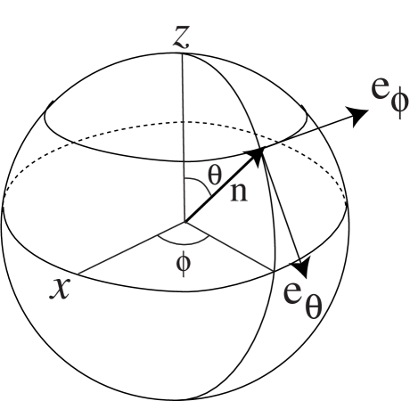
We use the standard definitions of polar coordinates and tangent vectors (see Fig. 7):

$${\bf n} = (\sin\theta\cos\phi,\sin\theta\sin\phi,\cos\theta)$$

$${\bf e}_{\theta} = (\cos\theta\cos\phi,\cos\theta\sin\phi,-\sin\theta)$$ (32)

$${\bf e}_{\phi} = (-\sin\phi,\cos\phi,0)$$

For the polarizer unit vector ${\bf s}$ with polar angles $(\theta_{s},\phi_{s})$ the scalar product expressions are

$$({\bf s}\cdot{\bf e}_{\theta}) = \sin\theta_{s}\cos\theta\cos(\phi_{s}-\phi)-\cos\theta_{s}\sin\theta$$

$$({\bf s}\cdot{\bf e}_{\phi}) = \sin\theta_{s}\sin(\phi_{s}-\phi)$$ (33)

References

- (1) L. Berger, J. Appl. Phys., 49, 2160 (1978); Phys. Rev. B 33, 1572 (1986); J.Appl.Phys. 63, 1663 (1988).
- (2) J.Slonczewski, J.Magn.Magn.Mater. 159, L1 (1996).
- (3) Ya. B. Bazaliy, B. A. Jones, and Shou-Cheng Zhang, Phys. Rev. B, 57, R3213 (1998).
- (4) A. Brataas, G. E. W. Bauer, and P. J. Kelly, Phys. Rep., 427, 157 (2006).
- (5) C. J. Garia-Cervera, Weinan E, J. Appl. Phys., 90, 370 (2001).
- (6) Ya. B. Bazaliy, Appl. Phys. Lett. 91, 262510, (2007).
- (7) Ya. B. Bazaliy, Phys. Rev. B 76, 140402(R), (2007).
- (8) Ya. B. Bazaliy, D. Olaosebikan, B. A. Jones, J. Nanoscience and Nanotechnology 8, 2891 (2008).
- (9) Ya. B. Bazaliy, Proceedings of SPIE Conference, Spintronics II, 7398, 73980P-1 (2009).
- (10) Ya. B. Bazaliy, B. A. Jones, and Shou-Cheng Zhang, Phys. Rev. B, 69, 094421 (2004).
- (11) J.C. Slonczewski, J. Magn. Magn. Mater. 247, 324 (2002)
- (12) Y. Zhou, S. Bonetti, C. L. Zha, and J. Akerman, New Journ. Phys. 11, 103028 (2009).
- (13) P.-B. He, R.-X. Wang, Z.-D. Li, Q.-H. Liu, A.-L. Pan, Y.-G. Wang, and B.-S. Zou, Eur. Phys. J. B 73, 417 (2010).
- (14) I. Sodemann and Ya. B. Bazaliy, Phys. Rev. B. 84, 064422 (2011).