Dispersion relations for meson-proton and proton-proton forward elastic scattering

Abstract

An analysis of the data on forward $pp,\bar{p}p,\pi^{\pm}p$ and $K^{\pm}p$ scattering is performed making use of the single- and double-subtraction integral and comparing with derivative dispersion relations for amplitudes. Various pomeron and odderon models for the total cross sections are considered and compared. The real part of the amplitude is calculated via dispersion relations. It is shown that the integral dispersion relations lead to a better description of the data for $\sqrt{s}>$5 GeV. Predictions of the considered models for the TOTEM experiment at LHC energies are given.

1 Introduction

High-energy hadron interactions in a soft kinematical region (low or zero transferred momenta) were and still are an important area of interest for experimentalists and theoreticians. One of the first tasks of all accelerators always is the measurement of the total and differential cross sections at small scattering angles. The TOTEM experiment [1] is running at the LHC to measure first of all the total $pp$ cross section at energies 7 TeV and 14 TeV and secondly the differential cross section of $pp$ scattering in quite a large interval of scattering angle. From the theoretical point of view, soft physics is beyond the reach of the perturbative methods of QCD. The most successful theoretical approach for a description of the various soft hadron processes is the theory of the analytic $S-$matrix and the methods of complex angular momentum. There are many important results in $S-$matrix theory that have a general character and do not depend on additional assumptions such as the existence of the Regge poles. Very useful examples of such results are the dispersion relations (DR) which the amplitude of hadron scattering must satisfy. The dispersion relations for the forward hadron-scattering amplitude is a subject of the special interest because it can be written in a form which relates measured quantities. Thus the dispersion relations can be used in two ways. If all terms in the DR can be calculated, then comparing it with the experimental data verifies the validity of analyticity, which is one of the main postulates of the theory. Alternatively, if for example some parameters are unknown, we can determine them by requiring the best agreement of DR with the corresponding experimental data. In what follows we show how the DR for the forward scattering of $pp,\bar{p}p,\pi^{\pm}p$ and $K^{\pm}p$ amplitudes must be applied to describe the experimental data on the total cross sections and the ratios of the real part to the imaginary part of amplitudes. We remind the reader of the main postulates and assumptions which are important in order to derive DR, describe the procedure for correctly using them, show the resulting description of the data and make predictions for measurements at LHC energies.

2 The main properties of the amplitude needed to derive DR

Mandelstam variables. The analytic $S$-matrix theory postulates that the amplitude of any hadronic process $ab\to cd$ is an analytic function of invariant kinematic variables.

$$s=(p_{a}+p_{b})^{2},\quad t=(p_{a}-p_{c})^{2},\quad u=(p_{a}-p_{d})^{2},\qquad s+t+u=m_{a}^{2}+m_{b}^{2}+m_{c}^{2}+m_{d}^{2}.$$ (1)

For the processes under interest $a^{\pm}p\to a^{\pm}p$ where $a=p,\pi,K,p^{-}\equiv\bar{p}$,

$$s+t+u=2(m_{a}^{2}+m_{p}^{2}).$$ (2)

Crossing symmetry. Crossing symmetry means that processes $a+p\longrightarrow a+p$ ($s$-channel), $a+\bar{a}\longrightarrow p+\bar{p}$ ($t$-channel) and $\bar{p}+p\longrightarrow a+\bar{a}$ ($u$-channel) are described by the limiting values of one analytic function $A(s,t,u)$ taken in different regions of the variables $s$, $t$ and $u$. Because only two of three variables $s$, $t$, $u$ are independent, in what follows we often write $A(s,t)$ instead of $A(s,t,u)$.

Structure of singularities. The main singularities of $ap$ and $\bar{a}p$ elastic scattering amplitudes at $t=0$ are shown in Fig.1. They are: i) the branch points at $s\geq(m_{a}+m_{p})^{2}$ corresponding to the threshold energies of elastic and inelastic processes, ii) branch points generated by the thresholds in $u$-channel at $s\leq 0$, iii) unphysical branch points (for elastic $\bar{a}p$ scattering) generated by $u$-channel states (at $4m_{\pi}^{2}\leq u\leq 4m_{p}^{2}$ ). Thus for amplitude we have the right-hand and the left-hand cuts shown in Fig. 1 (left).

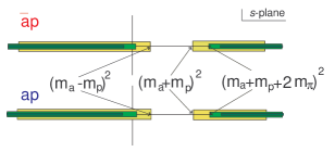
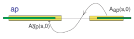
Figure 1: Structure of the singularities (left) and analytic continuation (right) of the $ap$ and $\bar{a}p$ elastic-scattering amplitudes

The physical amplitude of $ap$ elastic scattering is defined at the upper side of the all cuts from $(m_{a}+m_{p})^{2}$ to $+\infty$, i.e. $A_{ap}(s,t)=\lim\limits_{\varepsilon\to 0}A(s+i\varepsilon,t,u)\equiv A_{-}(s,t,u)$ at $s>(m_{a}+m_{p})^{2}$, $A_{\bar{a}p}(u,t)=\lim\limits_{\varepsilon\to 0}A(s,t,u+i\varepsilon)\equiv A_{+}(s,t,u)$ at $u>(m_{a}+m_{p})^{2}$. Furthermore, one can derive from the definition that

$$A_{\bar{a}p}(u,t)=\lim\limits_{\varepsilon\to 0}A(s-i\varepsilon,t,u)\quad\mbox{at}\quad s+t<0.$$ (3)

It follows from the above definitions that the amplitude $A_{\bar{a}p}$ can be obtained from $A_{ap}$ by analytic continuation as shown on the right-hand part of the Fig. 1.

The amplitudes can have poles at complex values of $s$ corresponding to resonances as well as branch points and corresponding unphysical cuts as for example at $s=4m_{\pi}^{2}$ in $\bar{p}p$ elastic scattering amplitude. Usually they are considered as small corrections at high energy.

Optical theorem. For $ap$ and $\bar{a}p$ it states that

$$\sigma_{tot}^{\bar{a}p}(s)\equiv\sigma_{+}=\frac{1}{2m_{p}p}ImA_{\bar{a}p}(s,0)=\frac{1}{2q_{s}\sqrt{s}}\,ImA_{+}(s,0),$$ (4)

$$\sigma_{tot}^{ap}(s)\equiv\sigma_{-}=\frac{1}{2m_{p}p}ImA_{ap}(s,0)=\frac{1}{2q_{s}\sqrt{s}}\,ImA_{-}(s,0)$$ (5)

where $p$ is the momentum of hadron $a$ in the laboratory system, $q_{s}$ is the relative momentum of $a$ and $p$ in the center-of-mass system, given by $q_{s}^{2}=\frac{1}{4s}[s-(m_{a}+m_{p})^{2}][s-(m_{a}-m_{p})^{2}]$ and $A_{\pm}(s,0)=A^{\bar{a}p}_{ap}(s,0)$.

Polynomial behaviour. It is well known that the scattering amplitude cannot rise at high $|s|$ faster than a power, i.e. $N$ must exist such that for $|s|\to\infty$ and $t_{0}<t\leq 0$

$$|A(s,t)|<|s|^{N}.$$ (6)

High-energy bounds for cross-sections. Total hadron cross sections behave at asymptotic energies in accordance with the well- known Froissart-Martin-Łukaszuk bound

$$\sigma_{t}(s)<\frac{\pi}{m_{\pi}^{2}}\ln^{2}(s/s_{0})\quad\mbox{at}\quad s\to\infty,\quad s_{0}\sim 1\ \mbox{GeV}^{2}.$$ (7)

The last inequality means that $|A(s,0)/s^{2}|\to 0\quad{\rm for}\ |s|\to\infty$. i.e. $N<2$ in Eq. (6).

3 Integral Dispersion Relations (IDR)

As an analytic function of the variable $s$, the amplitude $A(s,t)$ (in what follows we consider forward scattering amplitude, $t=0$) must satisfy the dispersion relation which can be derived from Cauchy’s theorem for analytic functions:

$$f(z)=\frac{1}{2\pi i}\oint\frac{f(z^{\prime})}{z^{\prime}-z}$$ (8)

where the contour $C$ surrounds the point $z$ and any singularity of $f(z)$ inside.

Because hadronic amplitudes $|A(s,0)/s^{2}|\to 0$ while $|A(s,0)/s|\nrightarrow 0$ at $|s|\to\infty$, it is more convenient to apply Cauchy’s theorem to the function $A(s,0)/((s-s_{0})(s-s_{1}))$ rather than directly to the amplitude. Generally, the points $s_{0}$ and $s_{1}$ are arbitrary but usually they are chosen at $s_{0}=s_{1}=2m_{p}^{2}$.

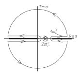
Figure 2: Deformation of an integration contour in the Cauchy integral for $A(s,0)$

Deforming the integration contour $C$ as shown in Fig. 2 in Cauchy’s theorem (more details can be found in the books [2, 3, 4]), and taking the circle to an infinite radius, so that its integral tends to $0$ (because $|A(s,0)/s^{2}|\to 0$ at $|s|\to\infty$), one can write

$$A(s,0)= A(s_{0},0)+(s-s_{0})A^{\prime}(s_{0},0)+\frac{(s-s_{0})^{2}}{2\pi}\bigg{[}\int\limits_{s_{tr}}^{\infty}\frac{D_{s}(s^{\prime},0)}{(s^{\prime}-s_{0})^{2}(s^{\prime}-s)}ds^{\prime}+\int\limits_{-\infty}^{\tilde{s}_{tr}}\frac{D_{s}(s^{\prime},0)}{(s^{\prime}-s_{0})^{2}(s^{\prime}-s)}ds^{\prime}\bigg{]}$$

$$= A(s_{0},0)+(s-s_{0})A^{\prime}(s_{0},0)+\frac{(s-s_{0})^{2}}{2\pi}\bigg{[}\int\limits_{s_{tr}}^{\infty}\frac{D_{s}(s^{\prime},0)}{(s^{\prime}-s_{0})^{2}(s^{\prime}-s)}ds^{\prime}+\int\limits_{s_{tr}}^{\infty}\frac{D_{u}(u^{\prime},0)}{(u^{\prime}-u_{0})^{2}(u^{\prime}-u)}du^{\prime}\bigg{]}$$ (9)

where $s_{tr}=(m_{a}+m_{p})^{2},\tilde{s}_{tr}=(m_{a}-m_{p})^{2}$ for the amplitudes $A_{ap}^{\bar{a}p}(s,0)$ and

$$D_{s}(s,t)=\frac{1}{i}[A(s+i\epsilon,t,u)-A(s-i\epsilon,t,u)],\qquad D_{u}(u,t)=\frac{1}{i}[A(s,t,u+i\epsilon)-A(s,t,u-i\epsilon)]$$ (10)

are the discontinuities of the amplitude accross the cuts.

After some simple transformations one can obtain the standard form of the integral dispersion relations written in the laboratory system ($s=2m_{p}(E+m_{p}),u=2m_{p}(-E+m_{p})$, the point $s_{0}=u_{0}$ corresponding to $E_{0}=0$ ):

$$\rho_{\pm}\sigma_{\pm}=\frac{A_{\pm}(s_{0},0)}{2m_{p}p}+\frac{E\,A_{\pm}^{\prime}(s_{0},0)}{p}+\frac{E^{2}}{\pi p}{\rm P}\int\limits_{m_{a}}^{\infty}\left[\frac{\sigma_{\pm}}{E^{\prime 2}(E^{\prime}-E)}+\frac{\sigma_{\mp}}{E^{\prime 2}(E^{\prime}+E)}\right]p^{\prime}\,dE^{\prime}$$ (11)

where $\rho_{\pm}=ReA_{\pm}(s,0)/ImA_{\pm}(s,0)$, $A^{\prime}(z,0)=dA(z,0)/dz$, $s_{0}=(m_{a}+m_{p})^{2}$ and

$$A_{+}(s_{0})=A_{-}(s_{0}),\qquad A^{\prime}_{+}(s_{0})=-A^{\prime}_{-}(s_{0}).$$ (12)

We would like to note that in reviews on high-energy physics [5] and [6] the dispersion relation with two subtractions contains missprints. Namely, in [5] the indexes “$pp$” and “$\bar{p}p$” must be rearranged in the integrands of the Eqs. (4.85) and (4.86). In the Eqs. (203) and (204) the sign “-” in the integrand must be replaced for the “+”.

It was confirmed by the COMPETE analysis [7], as well as in [8], that there are no indications of an odderon contribution to $\sigma_{tot}(s)$ and $\rho(s)$. This means that $\Delta\sigma_{t}(s)=\sigma_{t}^{(\bar{a}p)}(s)-\sigma_{t}^{(ap)}(s)\to 0$ at $s\to\infty$. If this is so, one should not apply the IDR in the form of Eq. (11) with free unknown constants $A(s_{0}),A^{\prime}(s_{0})$ even if $\sigma_{t}^{(a^{\pm}p)}(s)\propto\ln^{2}s$, i.e. $|A(s,0)|\propto s\ln^{2}s$ .

Indeed, let us consider the relation (11), insert $E$ in the integrand and write it as $(E-E^{\prime})+E^{\prime}$ in the first term and $(E+E^{\prime})-E^{\prime}$ in the second one. After simple transformations we obtain

$$\begin{array}[]{lll}\rho_{\pm}\,\sigma_{\pm}&=&\displaystyle\frac{1}{p}\left\{A_{\pm}(s_{0},0)/2m_{p}+E\,\left[A_{\pm}^{\prime}(s_{0},0)\mp\frac{1}{\pi}\int\limits_{m_{a}}^{\infty}\frac{\sigma_{+}-\sigma_{-}}{E^{\prime 2}}p^{\prime}\,dE^{\prime}\right]\right\}\\ &+&\displaystyle\frac{E}{\pi p}{\rm P}\int\limits_{m_{a}}^{\infty}\left[\frac{\sigma_{\pm}}{E^{\prime}(E^{\prime}-E)}-\frac{\sigma_{\mp}}{E^{\prime}(E^{\prime}+E)}\right]p^{\prime}\,dE^{\prime}.\end{array}$$ (13)

Now one can show that if $\Delta\sigma=\sigma_{+}-\sigma_{-}\to 0$ then

$$A_{\pm}^{\prime}(s_{0},0)=\pm\frac{1}{\pi}\int\limits_{m_{a}}^{\infty}\frac{\sigma_{+}-\sigma_{-}}{E^{\prime 2}}p^{\prime}\,dE^{\prime}.$$ (14)

This can be proven taking into account that $\sigma_{+}(s^{\prime})-\sigma_{-}(s^{\prime})=(-i/4m_{p}p^{\prime})[A^{(-)}(s^{\prime}+i\varepsilon)-A^{(-)}(s^{\prime}-i\varepsilon)]$, where $A^{(-)}(s)$ is the crossing-odd part of the amplitudes $A_{\pm}(s)$

$$A_{+}(s)\pm A_{-}(s)=2A^{(\pm)}(s).$$ (15)

Thus, if the odderon does not contribute to the amplitudes $A_{ap}^{\bar{a}p}(s,0)$ then the constants $A^{\prime}_{\pm}(s_{0},0)$ cannot be considered as free parameters, and their values can be calculated explicitly. Furthermore the IDR of the Eq.(11) is reduced to the form

$$\rho_{\pm}\,\sigma_{\pm}=\frac{A_{\pm}(s_{0},0)}{2m_{p}p}+\frac{E}{\pi p}{\rm P}\int\limits_{m_{p}}^{\infty}\left[\frac{\sigma_{\pm}}{E^{\prime}(E^{\prime}-E)}-\frac{\sigma_{\mp}}{E^{\prime}(E^{\prime}+E)}\right]p^{\prime}\,dE^{\prime}$$ (16)

which is the IDR with one subtraction. Dispersion relations of this form were first applied to data analysis by P. Söding [9] in 1964. It was then believed in that cross sections go to a constant at asymptotic energies. Therefore an application of the IDR with one subtraction was completely justified. But now we know that cross sections are rising with energy. Moreover, if we want to check the odderon hypothesis within the IDR method, we must use the relation (11) at least for $pp$ and $\bar{p}p$ cross sections and $\rho$ ratios. Note that because of its negative P-parity, the odderon does not contribute to meson-nucleon amplitudes. Hence for $\pi p$ and $Kp$ amplitudes we have to use the IDR (16) with one substraction.

4 Phenomenological application of the IDR for meson-proton and proton-proton forward- scattering amplitudes

We consider three explicit models for high-energy $p^{\pm}p,\pi^{\pm}p,K^{\pm}p$ total cross sections and corresponding $\rho$ ratios calculated through integral dispersion relations. We compare two possibilities for $p^{\pm}p$ cross sections, with and without an odderon contribution. In the first case, the IDR with two subtractions, Eq.(11), is used to calculate $\rho_{pp}$ and $\rho_{\bar{p}p}$, while in the second case the IDR with one subtraction, Eq.(16), is applied to calculate all $\rho$ ratios.

4.1 Low-energy part of the dispersion integral.

A high-energy parametrizations for the total cross sections based on the three pomeron models describe the data (all data used for presented analysis are taken from the standard set of the Particle Data Group [11]) at $\sqrt{s}\geq\sqrt{s_{min}}$= 5 GeV well. However, in order to calculate $\rho(s)$, we have to integrate the total cross sections from the threshold up to infinity. Thus we need an analytic form for the total cross sections at low energy. Therefore, we parametrize the cross sections for each process at low energies by some function which can have any number of parameters. The main aim is to describe the data as well as possible. Then when the high-energy data are fitted to in the various pomeron models, all these low-energy parameters are fixed. We only slightly change the low-energy parameterization to ensure continuity of the cross sections at the point $s=s_{min}$. Thus, in the low-energy parametrization we keep one free parameter for each cross section. The details of the parametrization of low-energy cross section play an auxiliary role and do not influence the results at $\sqrt{s}\geq\sqrt{s_{min}}$. The quality of the data description is quite good as can be seen from Fig.3.

However we would like to comment on the obtained $\chi^{2}/N_{p}$ ($\approx$ 3.9 for the whole set of data (number of points $N_{p}$=1932). The data are strongly spread around the main group of points, as it is seen from the Fig.4. There are a few points deviating quite far from them, and some of these points (for example in the $pp$ set only 6 points) individually contribute more than 40 to $\chi^{2}$ . If we exclude their contribution we obtain a reasonable value $\chi^{2}/N_{p}\approx 1.5$. In our opinion this quality of data description is acceptable in order to have a sufficiently precise value of the dispersion integral from the threshold to $\sqrt{s}$=5 GeV.

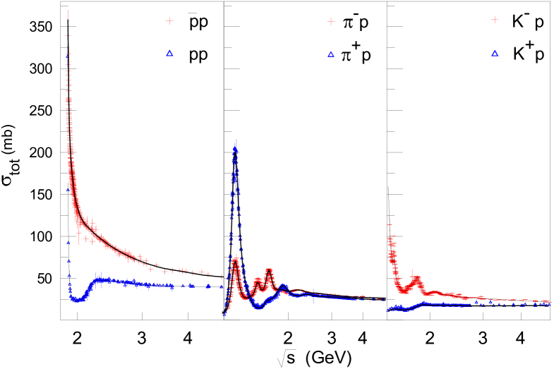
Figure 3: Description of the low-energy cross sections.

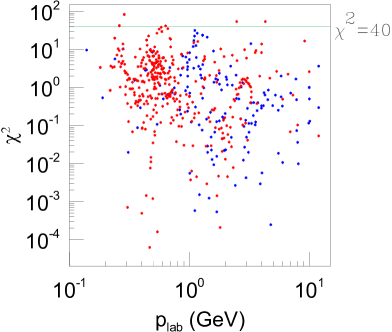
Figure 4: $\chi^{2}$ in the fit of the low-energy $pp$ and $\bar{p}p$ cross sections.

4.2 High-energy pomeron models.

We consider three models leading to different asymptotic behavior for the total cross sections. We start from the explicit parameterization of the total $pp$ and $\bar{p}p$ cross sections, then, to find the ratios of the real part to the imaginary part, we apply the IDR making use of the above-described parameterizations and calculating the low-energy part of the dispersion integral.

All the models include the contributions of the pomeron ${\cal P}$, of crossing-even and crossing-odd reggeons R (we consider these two reggeons as effective ones to avoid increasing the number of parameters as would be the case if we included the full set of secondary reggeons, $f,\omega,\rho,a_{2}$) and of the odderon (for $pp$ and $\bar{p}p$).

$$ImA_{ap}^{\bar{a}p}(s,0)={\cal P}(z)+{\cal R}_{+}(z)\pm{\cal R}_{-}(z)\pm{\cal O}(z),$$ (17)

$${\cal R}_{\pm}(z)=g_{\pm}z^{\alpha_{\pm}(0)},$$ (18)

$$z=|\cos\vartheta_{t}|=\frac{t+2(s-m_{p}^{2}-m_{a}^{2})}{\sqrt{(4m_{p}^{2}-t)(4m_{a}^{2}-t)}}=\frac{t+4Em_{p}^{2}}{\sqrt{(4m_{p}^{2}-t)(4m_{a}^{2}-t)}}$$ (19)

where $\vartheta_{t}$ is the scattering angle in the cross channel. If $t=0$ then $z=E/m_{a}$.

Simple-pole-pomeron model (SP). In this model, the intercept of the pomeron is larger than unity. In contrast with well-known Donnachie-Landshoff model [10], we add in the amplitude a simple pole (with $\alpha_{\cal P}(0)=1$) contribution

$${\cal P}(E)=g_{0}z+g_{1}z^{\alpha_{\cal P}(0)}.$$ (20)

In this model, we write the odderon contribution in the form

$${\cal O}(E)=g_{od}z^{{\alpha_{\cal O}(0)}},\quad\alpha_{\cal O}(0)\leq\alpha_{\cal P}(0).$$ (21)

Dipole-pomeron model (DP). The pomeron in this model is a double pole in the complex-angular-momentum plane with intercept $\alpha_{{\cal P}}(0)=1$.

$${\cal P}(E)=g_{0}z+g_{1}z\ln z,$$ (22)

$${\cal O}(E)=g_{od}z.$$ (23)

Tripole-pomeron model (TP). This pomeron is the hardest complex $j$-plane singularity allowed by unitarity, it is a pair of branch points which collide when $t\to 0$ and produce a triple pole at $j=1$

$${\cal P}(E)=g_{0}z+g_{1}z\ln z+g_{2}z\ln^{2}z.$$ (24)

$${\cal O}(E)=g_{1od}z+g_{2od}z\ln z.$$ (25)

The real part of amplitude can be calculated in two ways. It is obtained either by IDR (for $pp$ and $\bar{p}p$, with Eq. (11) if the odderon is taken into account and with Eq.(16) if not, or by the derivative-dispersion-relation method (alternatively one can use explicit parameterizations for both the imaginary part and the real part of the amplitude). Here we present the results for the IDR method. The second method is discussed and used in [12, 13, 15].

We can compare the fits using IDR with those based on standard asymptotic expressions for the amplitudes. These are built as follows. The contribution of Regge poles of signature $\tau$ ( +1 or -1) to the amplitude is

$$A_{R_{\tau}}(s,0)=\eta_{\tau}(\alpha_{R}(0))g_{R}z_{t}^{\alpha_{R}(0)}$$ (26)

where $\eta_{\tau}(\alpha_{R})$ is the signature factor

$$\eta_{\tau}(\alpha_{R})=\frac{1+\tau\exp(-i\pi\alpha_{R})}{-\sin(\pi\alpha_{R})}=\left\{\begin{array}[]{l}-\exp(-i\pi\alpha_{R}/2)/\sin(\pi\alpha_{R}/2),\quad\tau=+1,\\ -i\exp(-i\pi\alpha_{R}/2)/\cos(\pi\alpha_{R}/2),\quad\tau=-1.\end{array}\right.$$ (27)

The pomeron, odderon and reggeon contributions to the $pp,\ \bar{p}p$ scattering amplitudes due to the form (27) of the signature factor can be written as follows

$$\begin{array}[]{lll}A^{\bar{a}p}_{ap}(s,0)&=&-{\cal P}(-i\tilde{s})-{\tilde{R}}_{+}(-i\tilde{s})\mp i{\tilde{R}}_{-}(-i\tilde{s})\mp i{\tilde{\cal O}}_{-}(-i\tilde{s})\end{array}$$ (28)

where $\tilde{s}=s/s_{0},s_{0}=1$ GeV² and

$$\tilde{R}_{\pm}(-i\tilde{s})=\left\{\begin{array}[]{l}{\cal R}_{+}(-i\tilde{s})/\sin(\pi\alpha_{+}/2),\quad\tau=+1,\\ {\cal R}_{-}(-i\tilde{s})/\cos(\pi\alpha_{-}/2),\quad\tau=-1.\end{array}\right.$$ (29)

The odderon contribution ${\cal O}$ has a similar form if it is chosen as a simple pole. An advantage of the presentation (28) is that the cross sections in the models (18) and (29) have the same form. If the asymptotic normalization $\sigma_{t}(s)=ImA(s,0)/s)$ is chosen then Eq. (28) is a standard analytic parametrization in its asymptotic form. We denote a fit with such expressions for the amplitudes as a “$-is$ fit”.

We present here the results of the fit using IDR with the standard optical theorem (4) and briefly compare it with “$-is$” fits.

5 Fit results.

5.1 The experimental data and the fitting procedure.

We apply the dispersion relation method to the description and analysis of experimental data not only for $pp$ and $\bar{p}p$ total cross sections and ratios of the real part to the imaginary part of the forward scattering amplitudes. This has been done in the number of papers [6, 12, 13, 14, 15, 16, 17] (see also refs in these papers). We consider here additionally $\pi^{\pm}p$ and $K^{\pm}p$ data. All the data are taken from the standard set [11]. There are 411 points for total cross sections $\sigma_{t}^{a^{\pm}p}(s)$ and 131 points for ratios $\rho^{a^{\pm}p}(s)$ at $\sqrt{s}\geq$ 5 GeV.

5.2 The odderon contribution.

The odderon terms defined in Eqs.(21,23,25) in the corresponding pomeron models give small contribution to the $pp$ and $\bar{p}p$ cross sections. At LHC energies, the Reggeon contributions ${\cal R}_{\pm}$ are negligible, therefore $\Delta\sigma_{t}=\sigma_{t}^{\bar{p}p}-\sigma_{t}^{pp}$ is dominated by the odderon contribution. The fit to the data shows that the odderon contribution to the imaginary part of the forward scattering $pp$ and $\bar{p}p$ amplitude is very small. However, the real part of the odderon contribution is about 10% of the real part of the pomeron contribution, which can calculated at high energy as follows

$$\lambda=\frac{\rho_{\bar{p}p}\sigma_{t}^{\bar{p}p}-\rho_{pp}\sigma_{t}^{pp}}{\rho_{\bar{p}p}\sigma_{t}^{\bar{p}p}+\rho_{pp}\sigma_{t}^{pp}}=\frac{ReA^{(-)}}{ReA^{(+)}}.$$ (30)

The behavior of $\Delta\sigma$ and of $\lambda$ at energies $\sqrt{s}>$25 GeV are shown in Fig. 5 and Fig. 6. One can barely see a very small odderon contribution to the total cross section: ($\Delta\sigma/\sigma\leq 0.5\%$. Indeed, in the tripole-pomeron model $\sigma\propto\ln^{2}s$ and $\Delta\sigma\propto\ln s$). Nevertheless, Fig. 6 shows that the contribution of the odderon to the real part of the amplitudes in the TeV-energy region is sizeable (about 10%). The tripole-pomeron model is shown as an example, as the dipole- and simple-pole pomeron models show the same odderon effects.

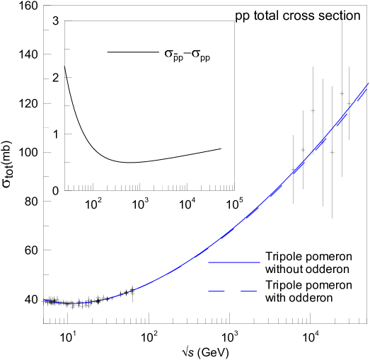
Figure 5: Tripole pomeron model with and without Odderon contribution.

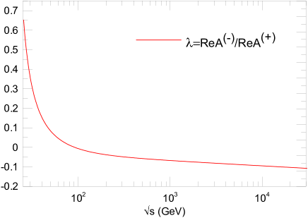
Figure 6: The odderon contribution to the real part of the amplitude in the tripole pomeron model at high energy.

However, comparing the values of the $\chi^{2}$ obtained in the considered models, one can conclude that the odderon contribution is not significant for data at $t=0$. The values of the $\chi^{2}/dof$ obtained in the considered models are given in the Table 1.

Table 1: The values of $\chi^{2}/dof$ in three pomeron models with and without odderon contribution

	$\chi^{2}/dof$
	Simple pole pomeron	Dipole pomeron	Tripole pomeron
With odderon	0.974	0.974	0.960
No odderon	0.976	0.974	0.963

5.3 Models without an odderon.

The quality of the data description in terms of $\chi^{2}/dof$ are again given in the Table 1, the parameters of the models are presented at the Table 2, comparison of the theoretical curves and the data are in the Figs. 7, 8, 9 for total cross sections and in the Figs. 10, 11, 12 for the ratios of real to imaginary part.

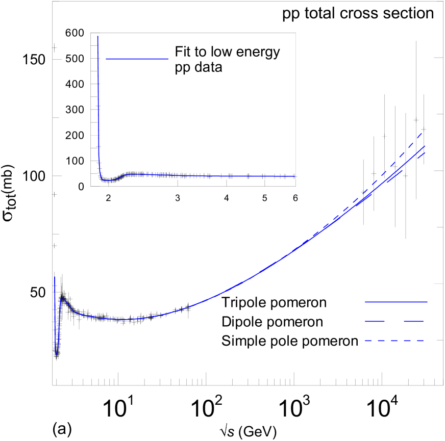
Figure 7: Total $pp$ (a) and $\bar{p}p$ (b) cross sections

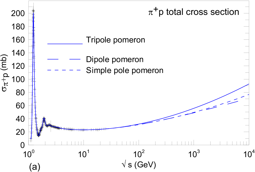
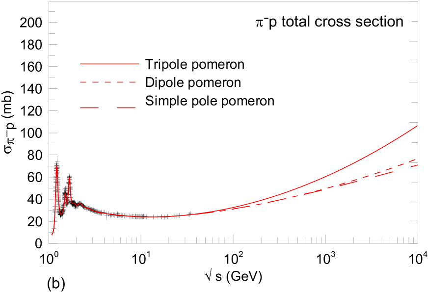
Figure 8: Total $\pi^{+}p$ (a) and $\pi^{-}p$ (b) cross sections

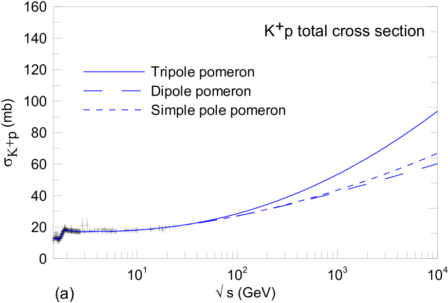
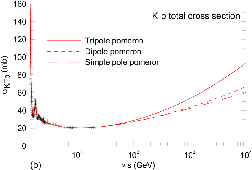
Figure 9: Total $K^{+}p$ (a) and $K^{-}p$ (b) cross sections

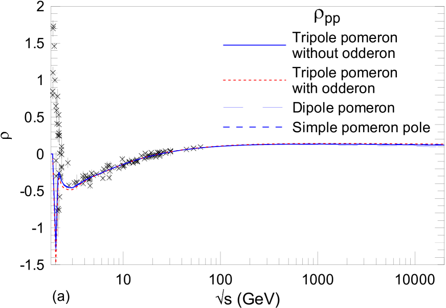
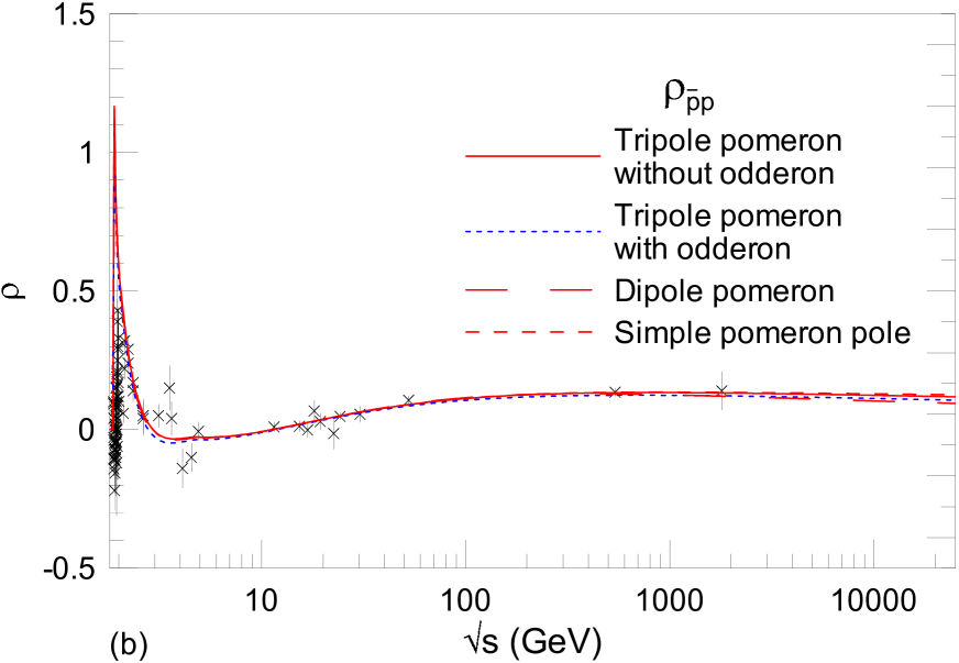
Figure 10: Ratio of real part to imaginary part of $pp$ (a) and $\bar{p}p$ (b) forward scattering amplitudes

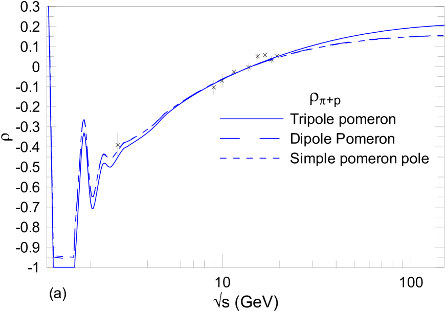
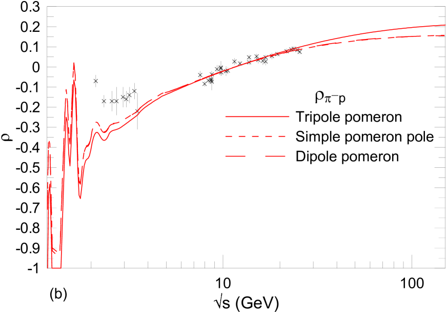
Figure 11: Ratio of real part to imaginary part of $\pi^{+}p$ (a) and $\pi^{-}p$ (b) forward scattering amplitudes

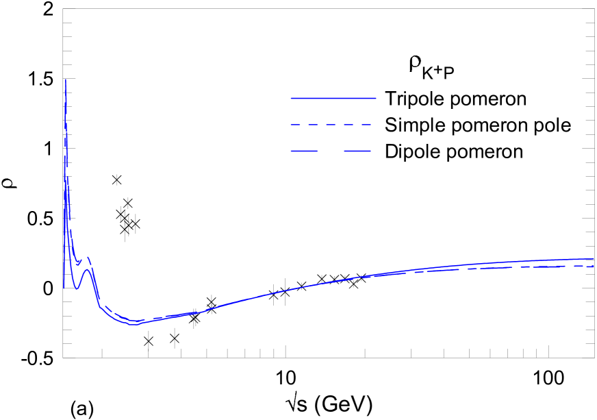
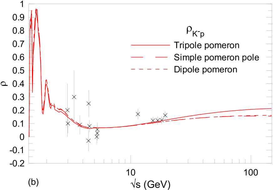
Figure 12: Ratio of real part to imaginary part of $K^{+}p$ (a) and $K^{-}p$ (b) forward scattering amplitudes

Table 2: The values of parameters obtained in the IDR fit for three pomeron models.

	Simple pole pomeron		Dipole pomeron		Triple pomeron
	value	error	value	error	value	error
Pomeron
$\alpha_{\cal P}(0)$	1.06435	0.00027	–	–	–	–
$g_{0p}$	-130.8	1.1	-136.7	1.2	122.00	0.23
$g_{1p}$	185.25	0.70	31.09	0.12	1.146	0.042
$g_{2p}$	–	–	–	–	0.9619	0.0060
$g_{0\pi}$	-20.659	0.095	-24.98	0.10	21.554	0.018
$g_{1\pi}$	20.184	0.060	3.607	0.010	-2.6941	0.0029
$g_{2\pi}$	–	–	–	–	0.25396	0.00041
$g_{0K}$	-59.91	0.40	-49.67	0.43	60.51	0.30
$g_{1K}$	66.32	0.25	10.231	0.049	-7.178	0.030
$g_{2K}$	–	–	–	–	0.8618	0.0028
$R^{+}$-Reggeon
$\alpha_{+}(0)$	0.7012	0.0018	0.80483	0.00069	0.6244	0.0011
$g_{+p}$	254.2	1.7	432.6	1.7	196.66	0.87
$g_{+\pi}$	41.22	0.31	62.05	0.19	13.11	0.12
$g_{+K}$	65.29	0.68	118.72	0.64	0.	490.
$R^{-}$-Reggeon
$\alpha_{-}(0)$	0.4726	0.0081	0.4734	0.0081	0.4725	0.0028
$g_{-p}$	103.3	3.3	102.9	3.3	103.4	1.3
$g_{-\pi}$	7.65	0.36	7.58	0.36	7.51	0.17
$g_{-K}$	30.6	1.1	30.5	1.1	30.50	0.52
Subtraction constants
$B_{p}$	-167.	33.	-172.	33.	-164.	30.
$B_{\pi}$	-78.	21.	-79.	21.	-89.	19.
$B_{K}$	13.	26.	14.	26.	6.	24.

One can see from the Figures that all the data at $\sqrt{s}>$ 5GeV are reproduced very well in all considered pomeron models. Nevertheless, they show (as should be because of the different asymptotic behavior) the different cross sections and ratios for the energies where there are no data yet. In Table 3 we compare predictions for the LHC energies obtained in three pomeron models, using three different methods for data analysis. The first one implements the IDR for all amplitudes, the second one is the standard “-is” fit with the asymptotic value of the flux factor in the optical theorem, and the third considers [17] only data on $pp$ and $\bar{p}p$ were analyzed. The values of $\chi^{2}/dof$ are shown as well for all cases.

Table 3: Predictions for the LHC energies of the considered pomeron models obtained within three methods of the fit. SP is the simple pole pomeron model, DP is the dipole pomeron model, TP is the tripole pomeron model.

	IDR, $a^{\pm}p,a=p,\pi,K$			“-is”, $a^{\pm}p,a=p,\pi,K$			IDR, $pp,\bar{p}p$
	SP	DP	TP	SP	DP	TP	SP	DP	TP
$\sqrt{s}=7$TeV
$\sigma_{t}$ (mb)	95.04	91.10	94.14	94.92	90.79	94.20	96.36	90.40	95.07
$\rho$	0.138	0.112	0.138	0.186	0.107	0.142	0.141	0.106	0.130
$\sqrt{s}=14$TeV
$\sigma_{t}$ (mb)	105.90	99.65	104.60	106.20	99.68	105.10	108.99	98.96	106.43
$\rho$	0.135	0.105	0.135	0.192	0.100	0.137	0.140	0.099	0.126
$\chi^{2}/dof$	0.976	0.974	0.963	1.14	0.998	0.984	1.096	1.103	1.096

Comparing the results obtained for $pp,\bar{p}p$ only with those for all processes we first note that the values of $\chi^{2}$ in the later fit are lower. Secondly, the predictions of three pomeron models in the later fit are closer to each other than those obtained from fitting $pp,\bar{p}p$ only. It seems, that the addition of the $\pi p$ and $Kp$ data restricts the freedom of the adjustable parameters of the models.

At the same time the curves $\rho$ for $\pi^{\pm}p$ and $K^{\pm}p$ at $\sqrt{s}<5$ GeV deviate significantly from the data. We would like to note that at low energies there is a well pronounced resonance structure in the $\pi^{\pm}p$ and $K^{\pm}p$ cross sections. It is well described by the low-energy parametrization (Section 4.1), but if the resonances contribute to the amplitudes, then they should be associated with poles of the amplitudes shifted from the real axis in the complex s-plane. Effectively they are taken into account in the imaginary part of amplitude, i.e. in the cross section. However they should contribute as well to the real part of amplitude. If we treat these resonances as stable strong interacting hadrons or as asymptotic states (in terms of S-matrix theory) we should add the residues of these poles to the IDR. This would lead to additional constants in the expressions for $ReA(s,0)$ in Eqs.(16), (11). Because of the different sets of the resonances for different processes, these constants must be not the same for $A_{a^{+}p}$ and $A_{a^{-}p}$ amplitudes. We tried to add such constants to the IDR but the decrease of $\chi^{2}$ (about 2-3%) and they do not improve an agreement with low-energy data. To explain these situation one should presumably argue that new branch points cuts, related to the production of the resonances and their subsequent decay into asymptotic particles, must be exist and must be taken into account in the IDR. These cuts are not important at high energy but they significantly contribute to the real part of amplitude at very low energy. This problem requires further investigation.

6 Conclusion

The method of integral dispersion relations leads to a better description of the high energy data, giving a $\chi^{2}/dof$ lower by a few percents than other methods, and to predictions similar to those obtained through other methods. LHC predictions of the each model from the three considered methods of analysis, we show the overall intervals for the predicted $pp$ cross section and $\rho$ ratios.

• Simple-pole pomeron model

  $$\sigma_{t}=\left\{\begin{array}[]{lll}\,\,\,\,94.9-\,\,\,\,96.4&\mbox{mb},&\sqrt{s}=\,\,\,\,{\rm 7\,\,TeV,}\\ 105.9-109.0&\mbox{mb},&\sqrt{s}={\rm 14\,\,TeV.}\\ \end{array}\right.\!\!\quad\rho=\left\{\begin{array}[]{ll}0.138-0.186,&\sqrt{s}=\,\,\,\,{\rm 7\,\,TeV,}\\ 0.135-0.192,&\sqrt{s}={\rm 14\,\,TeV.}\\ \end{array}\right.$$

• Double-pole pomeron model

  $$\sigma_{t}=\left\{\begin{array}[]{lll}90.4-91.1&\mbox{mb},&\sqrt{s}=\,\,\,\,{\rm 7\,\,TeV,}\\ 99.0-99.7&\mbox{mb},&\sqrt{s}={\rm 14\,\,TeV.}\\ \end{array}\right.\quad\rho=\left\{\begin{array}[]{ll}0.106-.112,&\sqrt{s}=\,\,\,\,{\rm 7\,\,TeV,}\\ 0.10-0.11,&\sqrt{s}={\rm 14\,\,TeV.}\\ \end{array}\right.$$

• Triple-pole pomeron model

  $$\sigma_{t}=\left\{\begin{array}[]{lll}\,\,\,\,94.1-\,\,\,\,95.1&\mbox{mb},&\sqrt{s}=\,\,\,\,{\rm 7\,\,TeV,}\\ 104.6-106.4&\mbox{mb},&\sqrt{s}={\rm 14\,\,TeV,}\\ \end{array}\right.\quad\rho=\left\{\begin{array}[]{ll}0.130-0.142,&\sqrt{s}=\,\,\,\,{\rm 7\,\,TeV,}\\ 0.126-0.137,&\sqrt{s}={\rm 14\,\,TeV.}\\ \end{array}\right.$$

If the precision of the TOTEM measurement of the total $pp$ cross section turns out to be better than 1% we will have a chance to select either DP model or SP and TP models (it seems from the total cross section only it would difficult to distinguish SP and TP models).

References

-
[1]
http://totem.web.cern.ch/Totem/ and references therein;
K. Eggert: Discussion Session EDS’09 - What can we learn / expect from the LHC Experiments? Proceedings of the 13th International Conference on Elastic and Diffractive Scattering (Blois Workshop) EDS 2009 - Moving Forward into the LHC Era, CERN-Proceedings-2010-002, ed. M. Deile et al., arXiv:1002.3527v1 [hep-ph]. - [2] P.D.B. Collins: An Introduction to Regge Theory and High Energy Physics, pp 460, Cambridge University Press (1977).
- [3] V. Barone, E. Predazzi: High-Energy Particle Diffraction, pp 419, Schpringer (2002).
- [4] S. Donnachie; P. Landshoff; O. Nachtmann; G. Dosch: Pomeron physics and QCD, pp 360, Cambridge University Press (2005).
- [5] M.M. Block, R.N. Cahn: High-energy and forward elastic scattering and total cross sections, Review of Modern Physics, 57, No 2, 563 (1985).
- [6] M.M. Block: Hadronic forward scattering: Predictions for the Large Hadron Collider and cosmic rays, Physics Report, 436, 71 (2006).
- [7] J.R. Cudell et al., (COMPETE Collab.): High-energy forward scattering and the pomeron: Simple pole versus unitarized models, Physical Review, D61, 034019 (2001). 612001034019; Hadronic scattering amplitudes: Medium-energy constraints on asymptotic behavior. Physical Review, D65, 074024 (2001): Benchmarks for the forward observables at RHIC, the Tevatron Run II and the LHC, Physical Revie Letters, 89, 201801 (2002).
- [8] M. Block, K. Kang: New limits on odderon amplitudes from analyticity constraints, Physical Review, D73, 094003 (2006).
- [9] P. Söding: Real part of the proton-proton and proton-antiproton forward scattering amplitude at high energies, Physics Letter, B8, 285 (1964).
- [10] A. Donnachie, P.V. Landshoff: Total Cross Sections, Physics Letter, B296, 227 (1992).
- [11] K. Nakamura et al. (Particle Data Group): The Review of Particle Physics, Journal of Physics, G 37, 075021 (2010), http://pdg.lbl.gov/.
- [12] E. Martynov, J.R. Cudell, Oleg V. Selyugin: Integral and derivative dispersion relations in the analysis of the data on and forward scattering, Ukrainian Journal of Physics, 48, 1274 (2003).
- [13] E. Martynov, J.R. Cudell, Oleg V. Selyugin: Integral and derivative dispersion relations, analysis of the forward scattering data, European Physics Journal, C 33, S533 (2004)
- [14] J.R. Cudell, E. Martynov, O. Selugin, A. Lengyel: The hard pomeron in soft data. Physics Letters, B587, 78 (2004) .
- [15] R.F. Avila, M.J. Menon: Derivative dispersion relations above the physical threshold, Brazilian Journal of Physics, 37, 358, (2007).
- [16] M. Ishida, K. Igi: Test of universal rise of hadronic total cross sections based on pi p, K p, anti-p p and p p scatterings, Progress of Theoretical Physics,.Suppl.187, 297 (2011).
- [17] A. Alkin, E. Martynov: Predictions for TOTEM experiment at LHC from integral and derivative dispersion relations, e-Print: arXiv:1009.4373 [hep-ph].