Semiclassical Spectrum of Small Bose-Hubbard Chains: A Normal Form Approach

Abstract

We analyze the spectrum of the 3-site Bose-Hubbard model with periodic boundary conditions using a semiclassical method. The Bohr-Sommerfeld quantization is applied to an effective classical Hamiltonian which we derive using resonance normal form theory. The derivation takes into account the 1:1 resonance between frequencies of a linearized classical system, and brings nonlinear terms into a corresponding normal form. The obtained expressions reproduce the exact low-energy spectrum of the system remarkably well even for a small number of particles $N$ corresponding to fillings of just two particles per site. Such small fillings are often used in current experiments, and it is inspiring to get insight into this quantum regime using essentially classical calculations.

I Introduction

Recent experimental and theoretical progress in the field of ultracold quantum gases has stimulated many studies at the interface of traditionally different disciplines such as atomic physics, quantum optics and condensed matter physics providing an intriguing link to fundamental many-body problems exp1 ; Bloch . A specific, but yet particularly interesting topic is the quantum-to-classical correspondence in degenerate quantum gases such as the adiabaticity versus non-adiabaticity of the quantum dynamics of finite matter-wave systems RMP ; Dziarmaga ; Altland ; Gurarie ; Mathey ; Grandi ; Abdullaev ; Kamchatnov1 ; Kamchatnov2 ; Sacha ; Ahufinger ; ITorma .

The Bose-Hubbard model (BHM) which we study here is a hallmark of condensed matter theory, and was realized experimentally using ultracold quantum gases in optical lattices Bloch following an ingenious theoretical suggestion Zoller . At the same time, in the classical limit it is described by the celebrated Discrete Nonlinear Schrodinger Equation (DNLSE), which possesses both a rich statics and dynamics Eilbeck . Properties of the BHM at high fillings (many particles per site) are known to be well-reproduced by several semiclassical methods, such as the mean-field approximation Kevrekidis or the truncated Wigner approximation TWAZoller ; TWAP . At low fillings, one would generally expect semiclassical methods to be inapplicable. Interesting enough, in a two-site BHM it was shown recently Korsch ; Keeling that semiclassical quantization reproduces the quantum spectrum remarkably well. That is, when considering the classical limit of the BHM and applying e.g. the Bohr-Sommerfeld quantization to the classical action, one obtains (semi)classical energies which show a good quantitative agreement with the exact (quantum) energies. A similar approach has been taken for the case of the three- and five-site BHM Kolovsky , with significant insights into the qualitative properties of the quantum spectrum, but no explicit expressions for the semiclassical spectrum having been obtained, and a corresponding comparison of the quantum and semiclassical predictions is still missing.

As we show here, the multi-site BHM exhibits an intricate classical dynamics which renders the construction of an effective Hamiltonian, necessary for a corresponding semiclassical quantization, a nontrivial mathematical problem. Our approach for the derivation of an effective classical Hamiltonian relies on resonance normal form theory AKN . We note that the classical system linearized around its equilibrium can be represented as a collection of harmonic oscillators, the frequencies of these oscillators being doubly degenerate. A pair of oscillators with frequencies in resonance 1:1 to each other can be analyzed using normalization techniques. To this end one needs to apply a series of canonical transformations that bring the quadratic and quartic terms of the Hamiltonian to a normal form, thereby completely eliminating all cubic terms. The obtained normalized Hamiltonian, written in terms of action-angle variables, depends on a pair of classical actions, which can then be straightforwardly quantized.

We note that our use of the normalization technique is very similar to that exploited recently in the studies of the mean-field dynamics of a nonlinear Stimulated Raman Adiabatic Passage (STIRAP) process PRL_STIRAP ; PRA_STIRAP . In its simplest version, nonlinear STIRAP considers three uniform condensates: an atomic Bose-Einstein condensate (BEC) in its ground state and a molecular BEC in its ground and an excited state coupled by a laser fields (a theory for the non-uniform case has also been developed K_STIRAP ). Using a certain time-dependent sequence of laser pulses, it is possible to convert the atomic BEC into a ground-state molecular BEC without populating the molecular BEC in the excited state. From a mathematical point of view, the system is a Hamiltonian dynamical system with two degrees of freedom possessing a rich dynamics, including e.g. nonlinear instabilities due to 1:1 resonances. It is an interesting fact that exactly the same degeneracy influences the dynamics of small Bose-Hubbard chains, as we will show below.

In detail we proceed as follows. Section II describes our classical and quantum model. It contains a derivation of the effective classical Hamiltonian, its semiclassical quantization and a comparison with the exact numerical results for the spectra for both the weak and strong interaction regime. Section III provides our conclusions. The Appendix contains a discussion of the two-site Bose-Hubbard chain, where the difference between weak and strong interaction regimes becomes transparent.

II Classical and quantum model

Let us consider the 3-site Bose-Hubbard model with periodic boundary conditions i.e. a ring geometry

$$H=-J\sum\limits_{\langle i,k\rangle}(\hat{a}_{i}^{\dagger}\hat{a}_{k}+h.c.)+\frac{U}{2}\sum\limits_{l=1}^{3}\hat{a}_{l}^{\dagger}\hat{a}_{l}^{\dagger}\hat{a}_{l}\hat{a}_{l},$$ (1)

where the first sum runs over all the nearest neighbours. As discussed e.g. in Ref. Kolovsky , one may try to understand its spectrum using the quantization of a corresponding effective classical Hamiltonian which will be derived in the following. To apply a semiclassical quantization, we firstly slightly modify the BHM Hamiltonian, thereby writing it in a symmetrized form:

$$H=-J\sum\limits_{\langle i,k\rangle}(\hat{a}_{i}^{\dagger}\hat{a}_{k}+h.c.)+\frac{U}{2}\sum\limits_{l=1}^{3}(\hat{n}_{l}+\frac{1}{2})^{2},$$ (2)

where $\hat{n}_{l}=\hat{a}_{l}^{\dagger}\hat{a}_{l}$ is the particle number operator for the $l-th$ site. Since the total number of particles is constant, this modification introduces only a (uniform) shift of all energy levels. The classical limit is then obtained by introducing $c-numbers$ for the operators $\hat{n}_{l}$ in analogy to a classical coherent state formalism $\hat{n}_{l}+\frac{1}{2}\to|\psi_{l}|^{2}$. This leads to the Discrete Nonlinear Schrödinger (DNLS) equation

$$H=-J\sum\limits_{\langle i,k\rangle}(\psi_{i}^{*}\psi_{k}+c.c.)+\frac{U}{2}\sum\limits_{l=1}^{3}|\psi_{l}|^{4},$$ (3)

$$i\frac{d\psi_{j}}{dt}=\frac{\partial H}{\partial\psi_{j}^{*}}=-J(\psi_{j+1}+\psi_{j-1})+U\psi_{j}|\psi_{j}|^{2},$$ (4)

It is important to note that the normalization of the classical amplitudes is $\sum_{i}|\psi_{i}|^{2}=N_{s}=N+\frac{3}{2}$, where $N$ is the total number of atoms in the quantum model Korsch . Introducing real pairs $(x_{n},y_{n})$ with $\psi_{n}=\frac{x_{n}+iy_{n}}{\sqrt{2}}$, the DNLSE is equivalent to the Hamiltonian equations of motion of the Hamiltonian

$$H=U\sum_{l=1}^{3}\frac{(x_{l}^{2}+y_{l}^{2})^{2}}{8}-J\sum_{\langle i,k\rangle}\left(x_{i}x_{k}+y_{i}y_{k}\right),$$ (5)

Switching to polar coordinates $x_{i}=\sqrt{2n_{i}}\sin\phi_{i},\quad y_{i}=\sqrt{2n_{i}}\cos\phi_{i}$, we arrive at the Hamiltonian

$$H=\frac{U}{2}\sum_{l=1}^{3}n_{l}^{2}-2J\sum_{\langle i,k\rangle}\left(\sqrt{n_{i}n_{k}}\cos(\phi_{i}-\phi_{k})\right),$$ (6)

with $\sum_{i}n_{i}=\mbox{const}=N_{s}=N+\frac{3}{2}$. We now perform a rescaling $n_{i}=I_{i}N_{s}$, $H=hN_{s}$. With $g=N_{s}U$ this leads to the Hamiltonian

$$h=\frac{g}{2}\sum_{l=1}^{3}I_{l}^{2}-2J\sum_{\langle i,k\rangle}\sqrt{I_{i}I_{k}}\cos(\phi_{i}-\phi_{k}),$$ (7)

with $\sum_{i}I_{i}=\mbox{const}=1.$

It is possible to introduce an effective classical Hamiltonian for the low-energy and high-energy dynamics of the system. Here we restrict ourselves to the low-energy part.

For $g>g_{cr}=-9/2$ the ground state is uniform in density and phase $I_{i}=1/3\hskip 5.69046pt\forall i$ and $\phi_{i}=\phi_{j}\hskip 5.69046pt\forall i,j$. For strongly attractive interaction $g<g_{cr}=-9/2$ the ground state is essentially different Eilbeck . Here we only consider values of interactions far from this bifurcation, i.e. we have $g>g_{cr}$.

II.1 Low-energy spectrum for small and moderate values of interaction

It is possible to eliminate one degree of freedom by applying a transformation with the generating function $W=p_{1}(\phi_{1}-\phi_{2})+p_{2}(\phi_{1}+\phi_{2}-2\phi_{3})/\sqrt{3}+p_{3}(\phi_{1}+\phi_{2}+\phi_{3})/3$.

This generating function is chosen such that the expressions occurring in the below-given Taylor expansion will have a simple appearance.

The transformed Hamiltonian depends only on two new phases $\theta_{1},\theta_{2}$ and their corresponding momenta $p_{1},p_{2}$, while the third momentum is an integral of motion $p_{3}=\sum_{i=1}^{3}I_{i}=1$. At values of $g$ larger than the critical value $g_{cr}$, the stable equilibrium is at the origin $p_{1,2}=0$, $\theta_{1,2}=0$. We expand our Hamiltonian around the origin up to terms of fourth-order power in coordinates and momenta. Without loss of generality we put $J=1$ in the following.

The resulting Hamiltonian is

$$h=h_{0}+\frac{\theta_{1}^{2}+\theta_{2}^{2}}{2}+\frac{9+2g}{2}(p_{1}^{2}+p_{2}^{2})+H_{3}+H_{4},$$ (8)

where $H_{3}$ and $H_{4}$ contain cubic and quartic terms, respectively, and $h_{0}=-2+\frac{g}{6}$ is a constant. Note that the quadratic part of the Hamiltonian describes two harmonic oscillators whose frequencies are in resonance 1:1. It is exactly this type of degeneracy which was recently considered in Ref. PRL_STIRAP ; PRA_STIRAP . The quadratic part of the Hamiltonian implies a bifurcation at $g_{cr}=-9/2$, i.e. at sufficiently strong attractive interaction. As already mentioned above, we focus on the low-energy dynamics off this bifurcation, i.e. for weakly attractive or repulsive interactions.

The cubic terms are given by

$$H_{3}=\frac{\sqrt{3}}{4}(2\theta_{1}\theta_{2}p_{1}+(\theta_{1}^{2}-\theta_{2}^{2}-27p_{1}^{2})p_{2}+9p_{2}^{3})$$ (9)

To bring the Hamiltonian to its normal form, we need to get rid of the cubic terms. This can be done by a nonlinear near-to-identity canonical transformation $p_{1,2},\theta_{1,2}\to P_{1,2},X_{1,2}$ determined by the generating function

$$W=\theta_{1}(P_{1}+\beta P_{1}P_{2})+\theta_{2}(P_{2}+\alpha P_{2}^{2}+\gamma P_{1}^{2}+c\theta_{1}^{2}+d\theta_{2}^{2}),$$ (10)

with the coefficients

$$\alpha=-\frac{9\sqrt{3}}{4A},\quad\beta=-2\alpha,\quad\gamma=-\alpha,$$ (11)

$$c=\sqrt{3}\frac{18-A}{4A^{2}},\quad d=-c/3,\quad A=9+2g$$ (12)

This transformation does not change the quadratic terms, removes the cubic terms, and modifies the quartic ones. We subsequently change to polar coordinates $J_{1,2},\Phi_{1,2}$, with $X_{1,2}=\sqrt{2J_{1,2}}A^{1/4}\sin{\Phi_{1,2}},P_{1,2}=\sqrt{2J_{1,2}}A^{-1/4}\cos{\Phi_{1,2}}$

In the resulting Hamiltonian, we keep only slowly varying terms which depend on $\Phi_{1}-\Phi_{2}$, and average out (i.e. omit) other (’fast’) trigonometric terms, e.g. $\cos 2\Phi_{1},\cos 2\Phi_{2},\cos(2(\Phi_{1}+\Phi_{2}))$, etc. We thus arrive to the normal form

$$H=\sqrt{A}(J_{1}+J_{2})+B(J_{1}^{2}+J_{2}^{2})+CJ_{1}J_{2}+DJ_{1}J_{2}\cos[2(\Phi_{1}-\Phi_{2})],$$ (13)

where

$$B = -\frac{3g}{8A^{2}}(54+24g+g^{2}),\quad C=-\frac{g}{2A^{2}}(6+g)(18+g),$$ (14)

$$D = -\frac{g}{4A^{2}}(-54+24g+g^{2}),$$ (15)

One can easily see that at $g=0$ all coefficients $B,C,D$ are equal to zero, implying the degeneracy of the Hamiltonian with respect to $J_{1}-J_{2}$ at this point. Introducing $J=\frac{J_{1}+J_{2}}{2},P=\frac{J_{1}-J_{2}}{2}$, we get the Hamiltonian

$$h=2\sqrt{A}J+2B(J^{2}+P^{2})+C(J^{2}-P^{2})+D(J^{2}-P^{2})\cos 2\Phi$$ (16)

where $P$ and $\Phi$ are canonically conjugate. This Hamiltonian is integrable, since $J=$const. $J$ is the first action variable of our effective Hamiltonian, the second one we find by calculating $K=\frac{1}{2\pi}\int Pd\Phi$. This integral can be calculated analytically, which provides us with an expression for $K(h)$. Inverting it, we finally find that

$$h=2\Omega J+cJ^{2}-e[K^{2}-2KJ],$$ (17)

where

$$c=2C=-\frac{g}{A^{2}}(6+g)(18+g),\quad e=D=-\frac{g}{4A^{2}}(-54+24g+g^{2}),\quad\Omega=\sqrt{A},$$ (18)

The above expression (17) together with the constants (18) constitute the main result of this paper. The quantization of the actions $J,K$ should reproduce the low-lying energy levels of the system. We use the following quantization of the actions

$$2J = \frac{n+1}{N_{s}},\quad n=0,1,..N,$$ (19)

$$2K = \frac{m+1/2}{N_{s}},\quad m=0,..n,$$ (20)

The resulting semiclassical energy-levels $E_{nm}$ are shown in Figs. 1, 2, in comparison with the results from exact numerical diagonalization for N=24 and N=6. It is observed that for moderate values of the interaction strength $|g|$ the exact spectrum is reproduced very well. To be more specific, there are two phenomena occuring for the spectrum with increasing $|g|$. At zero interaction the exact spectrum coincides with the Bogoliubov one, and the energy levels are organized in (degenerate) Bogoliubov bands. As $g$ is increased, these energy bands decrease and their degeneracy is lifted.

The first phenomenon is reproduced by the semiclassical approach remarkably well. That is, we see from Figs.1, 2 that the energetical distance between the exact solutions and the semiclassical prediction is much less than the distance between the exact and the linearized solutions (i.e., the deviation of the exact spectrum from the Bogoliubov frequencies is much larger than its deviation from the semiclassical prediction). At the same time, the spreading of the energy levels within the Bogoliubov band is reproduced not very well. For large $g$-values the deviation is considerable. As $g$ is increased, fluctuations with respect to the phase grow and an expansion around the classical ground state becomes inapplicable: the phase is not confined to the vicinity of 0 anymore. The case of large $g$ is analyzed in the next section.

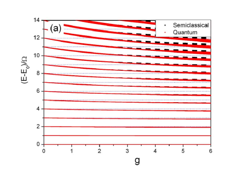
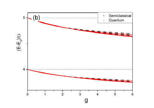
Figure 1: Energy levels of the three-site BHM (red solid lines) and semiclassical levels given by Eq. (17) (black dashed lines) as a function of the interaction strength $g$ for $N=24$ atoms. The energy levels are rescaled to the Bogoliubov frequencies, i.e. we show $(E-E_{0})/\Omega$, where $E_{0}$ is the energy of the ground state, and $\Omega=\sqrt{A}=\sqrt{9+2g}$. The Bogoliubov levels are denoted by blue dotted lines.

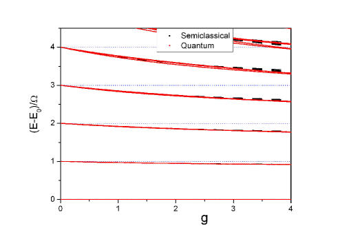
Figure 2: Energy levels of the three-site BHM (red solid lines) and semiclassical levels given by Eq. (17) (black dashed line) as a function of the interaction strength $g$ for $N=6$. The energy levels are rescaled to the Bogoliubov frequencies. The corresponding Bogoliubov levels are denoted by blue dotted lines.

II.2 Low-energy spectrum for strong interactions

At strong interactions, even though the classical ground state remains unchanged (uniform in density and phase), the semiclassical ground state becomes qualitatively different. The semiclassical ground state includes zero-point oscillations, i.e. the corresponding classical trajectories possess certain non-zero classical actions. With increasing interaction strength, the area of the phase space filled with trajectories oscillating around the classical ground state shrinks. At a certain value of $g$ the oscillatory area cannot accommodate trajectories with these minimal actions. As a result, the nature of the classical motion changes from oscillatory to rotational. In other words, the zero-point oscillations destroy the phase coherence. This is most easily illustrated for the double-well case (see supplementary information). One can consider it as a (semi)classical counterpart of the Mott-insulator transition. To be more precise, in finite quantum chains the Mott-insulator transition becomes a smooth crossover, and the change of the classical motion described above is the classical counterpart of this crossover.

From a technical point of view, this qualitative change in classical trajectories corresponding to the ground and low-lying states leads to the inapplicability of the fourth-order expansion of the classical Hamiltonian around the origin: phases now cover the interval $[-\pi,\pi)$ and are not restricted to the vicinity of zero. An adequate effective Hamiltonian will consequently change severely. To derive it, one can use classical perturbation theory such as Linstedt’s method AKN .

Similar to the case of weak interactions, we introduce

$$P_{1}=\frac{I_{1}-I_{2}}{2},\quad P_{2}=\frac{1}{6}(I_{1}+I_{2}-2I_{3}),\quad P_{3}=\sum\limits_{i=1}^{3}I_{i}=1,$$ (21)

Expanding the Hamiltonian in powers of $P_{1},P_{2}$ and $1/g$, one obtains

$$H=g[\frac{1}{6}+P_{1}^{2}+3P_{2}^{2}-\frac{2}{3g}(\cos\Phi_{1}+2\cos\frac{\Phi_{1}}{2}\cos\frac{\Phi_{2}}{2})+O(P_{i}/g)]$$ (22)

We assume that the interaction strength $g$ is large enough such that $P_{i}>\sqrt{1/g}$ holds. This holds if $1/N\gg\sqrt{1/g}$. Then, the classical dynamics takes place outside the resonance zones i.e. it becomes a rotational motion. Then, in the first approximation of Linstedt’s method, one introduces new actions $P_{1}\to J_{1},P_{2}\to J_{2}$, and the averaged Hamiltonian in the new actions $J_{1},J_{2}$ coincides with the unperturbed initial Hamiltonian (this result can be obtained by other methods as well Benetin ),

$$H=g[\frac{1}{6}+J_{1}^{2}+3J_{2}^{2}]$$ (23)

The semiclassical energy levels are obtained by quantizing $J_{1},J_{2}$:

$$E_{n_{1},n_{2}}=gN_{s}(\frac{1}{6}+j_{1}^{2}+j_{2}^{2}),j_{1}=\frac{n_{1}-n_{2}}{2N_{s}},\quad j_{2}=\frac{n_{1}+n_{2}}{2N_{s}}-\frac{1}{3},\quad n_{1}=0,..,N,\quad n_{2}=0,..,N-n_{1},$$ (24)

Fig.3 shows a comparison of the semiclassical and exact results. In the second approximation of Lindstedt’s method, the dependence of the new Hamiltonian on the actions is slightly modified and the corresponding expressions are more cumbersome and therefore not provided here.

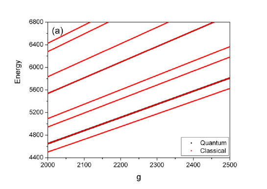
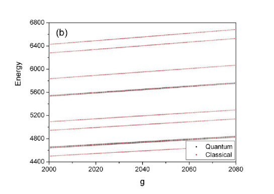
Figure 3: Energy levels of the three-site BHM (black squares) and semiclassical energy levels given by Eq. (24) (red circles) as a function of the interaction strength $g$. The levels are almost indistinguishable on the scale of (a). (b) represents an enlarged view of a part of (a).

III Concluding remarks

We have shown that by performing a proper analysis of the classical counterpart of a few-site Bose-Hubbard model one can gain valuable insights into the dynamics of the system.

The classical system possesses two degrees of freedom and its small-amplitude oscillations around the ground (equilibrium) state can be brought into the form of two decoupled linear oscillators. An important feature of the system is that the oscillators are in resonance 1:1 to each other. As a subsequent approximation, considering excitations on top of the ground state with larger amplitude, one should therefore apply resonance normal form theory. This allows us to bring the system to the form of an integrable nonlinear Hamiltonian depending on two classical actions. The quantum spectrum can then be reproduced by quantizing these actions. From the point of view of the physics of Bose-Einstein condensates, this procedure can be seen as an extension of the Bogoliubov transformations to the realm of nonlinear oscillations.

For strong interactions, the properties of the system change drastically. Here perturbation theory with respect to the inverse interaction strength leads to a system of uncoupled rotators.

An interesting dynamics occurs if one dynamically sweeps the interaction from strong to weak values (or vice versa), passing through the crossover region. Depending on the sweeping rate of the interaction, the crossover region is passed adiabatically or non-adiabatically and correspondingly different amounts of excitations are produced at the end of the sweep. This problem for the triple-well is left for future research. However, we solved it for the double-well. This allows, e.g, to construct a mathematical theory of slow decoupling of two superfluids, extending the results of Mathey on abrupt decoupling of superfluids to the case of slow sweeps. This question is presented elsewhere Schmelcher .

The results can be generalized to the case of longer chains. While it is understood that normal form theory is useful for weakly interacting wave dynamics Lvov , we are not aware about corresponding explicit calculations in BHM.

Appendix A Quantization of the two-site chain

For comparison, we consider here the quantization in case of the double-well problem. The two-site Bose-Hubbard Hamiltonian reads

$$\hat{H}=-J(\hat{a}_{2}^{\dagger}\hat{a}_{1}+\hat{a}_{1}^{\dagger}\hat{a}_{2})+\frac{U}{2}[\hat{n}_{1}(\hat{n}_{1}-1)+\hat{n}_{2}(\hat{n}_{2}-1)]$$ (25)

The symmetrized form of the interaction term is

$$\frac{U}{2}[(\hat{n}_{1}+\frac{1}{2})^{2}+(\hat{n}_{2}+\frac{1}{2})^{2}-\frac{1}{2}-2(\hat{n}_{1}+\hat{n}_{2})],$$ (26)

therefore we will consider below the slightly modified form of the BHM, additionally asuming $J=1$:

$$\hat{H}=-(\hat{a}_{2}^{\dagger}\hat{a}_{1}+\hat{a}_{1}^{\dagger}\hat{a}_{2})+\frac{U}{2}[(\hat{n}_{1}+\frac{1}{2})^{2}+\hat{(}\hat{n}_{2}+\frac{1}{2})^{2}]$$ (27)

The semiclassical limit is given by the Hamiltonian

$$H=-(\psi_{2}^{*}\psi_{1}+\psi_{1}^{*}\psi_{2})+\frac{U}{2}[|\psi_{1}|^{4}+|\psi_{2}|^{4}],$$ (28)

with the corresponding equations of motion

$$i\frac{d\psi_{j}}{dt}=\frac{\partial H}{\partial\psi_{j}^{*}},\quad i\frac{d\psi_{j}^{*}}{dt}=-\frac{\partial H}{\partial\psi_{j}}.$$ (29)

The normalization of the semiclassical variables is Korsch

$$|\psi_{1}|^{2}+|\psi_{2}|^{2}=N+1=N_{S}$$ (30)

Introducing $\psi_{i}=\frac{x_{i}+y_{i}}{\sqrt{2}}$, the equations of motion for $x_{i},y_{i}$ are determined by the classical Hamiltonian

$$H=\frac{U}{8}[(x_{1}^{2}+y_{1}^{2})^{2}+(x_{2}^{2}+y_{2}^{2})^{2}]-(x_{1}x_{2}+y_{1}y_{2}),$$ (31)

which after transforming $x_{i}=\sqrt{2I_{i}}\cos\phi_{i},\quad y_{i}=\sqrt{2I_{i}}\sin\phi_{i}$ becomes

$$H=\frac{U}{2}(I_{1}^{2}+I_{2}^{2})-2\sqrt{I_{1}I_{2}}\cos{(\phi_{1}-\phi_{2})}$$ (32)

with the integral of motion $I_{1}+I_{2}=N_{s}$. Employing the generating function $W=\frac{P}{2}(\phi_{1}-\phi_{2})+\frac{N_{s}}{2}(\phi_{1}+\phi_{2})$ to canonically transform the above Hamiltonian we arrive at

$$H=\frac{U}{4}(P^{2}+N_{s}^{2})-\sqrt{N_{s}^{2}-P^{2}}\cos 2\phi$$ (33)

Subsequently the transformation $P=N_{s}p$, $H=N_{s}h$, and gives us

$$h=\frac{gp^{2}}{4}-\sqrt{1-p^{2}}\cos 2\phi,$$ (34)

where $g=UN_{s}$. For weak interactions, a phase point oscillates around the ground state. For strong interactions, separatrix $h=$ shrinks to the vicinity of $p=0$, and when the area within the separatrix divided by $2\pi$ becomes less than the minimal action $\frac{1}{2N_{s}}$, nature of motion of the phase point corresponding to the semiclassical ground state changes: it is a rotation, with $\phi$ covering the full interval $(0,2\pi)$.

While it is not difficult to calculate the classical action here, we would like to follow a general scheme which could be generalized to a $M-site$ Bose-Hubbard chain. Therefore for weak interactions we proceed with an expansion of the Hamiltonian around its equilibrium, keeping terms of up to the fourth order. Expanding the Hamiltonian close to the origin, one gets

$$h=-1+2\phi^{2}+p^{2}(1+g/2)/2+\frac{p^{4}}{8}-p^{2}\phi^{2}-\frac{2\phi^{4}}{3}$$ (35)

The quadratic part can be transformed to action-angle variables easily

$$p=\sqrt{2I/\omega}\cos x,\quad\phi=\sqrt{2I\omega}\sin x,\quad\omega=\frac{1}{2}\sqrt{1+g/2}$$ (36)

Then we obtain

$$h=-1+\Omega I-\frac{g(8+g)}{4\Omega^{2}}I^{2}+I^{2}F(x),$$ (37)

where $\int\limits_{x=0}^{2\pi}F(x)=0$, $\Omega=4\omega=\sqrt{2(2+g)}.$ Averaging over $x$, we get the effective Hamiltonian

$$h=-1+\Omega I-\frac{g(8+g)}{4\Omega^{2}}I^{2}$$ (38)

The quantization of the action leads to $I_{n}=\frac{n+1/2}{N_{s}},\quad n=0,..N$ and finally gives us the semiclassical energy levels

$$E=N_{s}\left(\frac{g}{4}-1+\Omega I_{n}-\frac{g(g+8)I_{n}^{2}}{4\Omega^{2}}\right),$$ (39)

which reproduce the low-energy spectrum of the dimer BHM remarkably well even for $N\sim 10$ (see Fig. 4).

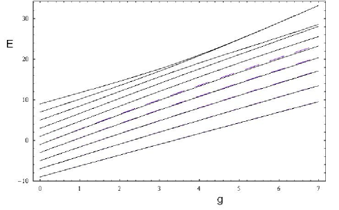
Figure 4: Energy levels of the two-site BHM (black solid lines) and the first 5 semiclassical levels (39) (blue dashed lines) for $N=9$ atoms. The first three levels are almost indiscernible on this scale.

References

- (1) I. Bloch, J. Dalibard, and W. Zwerger, Rev. Mod. Phys. 80, 885 (2008); S. Giorgini, L.P. Pitaevskii, and S. Stringari, ibid 80, 1215 (2008).
- (2) M. Greiner, O. Mandel, T. Esslinger, T.W. Hansch, and I. Bloch, Nature 415, 39 (2002).
- (3) Dziarmaga, Adv. Phys. 59, 1063 (2010).
- (4) A. Polkovnikov, L.Sengupta, A.Silva, M.Vengalattore, Rev. Mod. Phys. 83, 863 (2011).
- (5) A. Altland et al., Phys.Rev. A 79, 042703 (2009).
- (6) V. Gurarie, Phys. Rev. A 80, 023626 (2009).
- (7) L.Mathey, A.Polkovnikov, Phys. Rev. A 81, 033605 (2010).
- (8) C.De Grandi, A. Polkovnikov, in Lect. Notes Phys. 802, Eds. A. Chandra, B.K. Chakrabarti, Springer, Heidelberg, 2010.
- (9) F. Kh. Abdullaev et al, Phys. Rev. A 67, 013605 (2003).
- (10) F.Kh. Abdullaev, A.M. Kamchatnov, V.V. Konotop, and V.A. Brazhnyi, Phys. Rev. Lett 90, 230402 (2003).
- (11) T.L. Horng et al, Phys. Rev. A 79, 053619 (2009).
- (12) B.Damski, K.Sacha, J. Zakrzewski, J.Phys. B 35, 4051 (2002).
- (13) C.Ottaviani, V.Ahufinger, R.Corbaan, J. Mompart, Phys. Rev A 81, 043621 (2010)
- (14) A.P. Itin, P.Törmä, arXiv::0901.4778 (2010); A.P. Itin, P. Törmä, Phys. Rev. A 79, 055602 (2009).
- (15) D. Jaksch, C. Bruder, J. I. Cirac, C.W. Gardiner, and P. Zoller, Phys. Rev. Lett. 81, 3108 (1998).
- (16) J.C. Eilbeck, P.S. Lomdahl and A.C. Scott, Physica D 16, 318 (1985).
- (17) A. Smerzi, A. Trombettoni, P.G. Kevrekidis, A.R. Bishop, Phys. Rev. Lett. 89, 170402 (2002).
- (18) C.W. Gardiner and P. Zoller, Quantum Noise (Springer-Verlag, 2004).
- (19) A.Polkovnikov, Phys. Rev. A 68, 033609 (2003).
- (20) E.M. Graefe anf H.J. Korsch, Phys. Rev. A 76, 032116 (2007).
- (21) F. Nissen, J.Keeling, Phys. Rev. A 81, 063628 (2010).
- (22) A.R. Kolovsky, Phys. Rev. Lett 99, 020401 (2007); A.R. Kolovsky, Phys. Rev. E 76, 026207 (2007).
- (23) V.I. Arnold, V.V. Kozlov, and A.I. Neishtadt, Mathematical aspects of classical and celestial mechanics (Third Edition, Springer, Berlin, 2006).
- (24) A.P.Itin, S.Watanabe, Phys. Rev. Lett. 99, 223903 (2007).
- (25) A.P.Itin, S.Watanabe, and V.V. Konotop, Phys.Rev. A 77, 043610 (2008).
- (26) H.A. Cruz, V.V. Konotop, Phys. Rev. A 83, 033603 (2011).
- (27) G.Benettin, L. Galgani, A. Giorgilli, Nuovo Cimento B 89, 89 (1985).
- (28) A.P.Itin et al, in preparation.
- (29) V.S. L’vov, Wave turbulence under parametric excitation (Springer-Verlag, Berlin, 1994), chapter 1.