Source Coding When the Side Information May Be Delayed

Abstract

For memoryless sources, delayed side information at the decoder does not improve the rate-distortion function. However, this is not the case for sources with memory, as demonstrated by a number of works focusing on the special case of (delayed) feedforward. In this paper, a setting is studied in which the encoder is potentially uncertain about the delay with which measurements of the side information, which is available at the encoder, are acquired at the decoder. Assuming a hidden Markov model for the source sequences, at first, a single-letter characterization is given for the set-up where the side information delay is arbitrary and known at the encoder, and the reconstruction at the destination is required to be asymptotically lossless. Then, with delay equal to zero or one source symbol, a single-letter characterization of the rate-distortion region is given for the case where, unbeknownst to the encoder, the side information may be delayed or not, and additional information can be received by the decoder when the side information is not delayed. Finally, examples for binary and Gaussian sources are provided.

I Introduction

Consider a sensor network in which a sensor measures a certain physical quantity $Y_{i}$ over time $i=1,2,...n.$ The aim of the sensor is communicating a symbol-by-symbol processed version $X^{n}=(X_{1},...,X_{n})$ of the measured sequence $Y^{n}=(Y_{1},...,Y_{n})$ to a receiver. As an example, each element $X_{i}$ can be obtained by quantizing or denoising $Y_{i}$, for $i=1,2,...n.$ To this end, based on the observation of $X^{n}$ and $Y^{n}$, the sensor communicates a message $M$ of $nR$ bits to the receiver ($R$ is the message rate in bits per source symbol). The receiver is endowed with sensing capabilities, and hence it can measure the physical quantity $Y^{n}$ as well. However, as the receiver is located further away from the physical source, such measure may come with some delay, say $n+d$ for some $d\geq 0$. Assuming that at time $n+i$ the decoder must put out an estimate $Z_{i}$ of the $i$th source symbol $X_{i}$ by design constraints, it follows that the estimate $Z_{i}$ can be made to be a function of the message $M$ and of the delayed side information $Y^{i-d}=(Y_{1},...,Y^{i-d})$ (see [1] for an illustration). Following related literature (e.g., [2]), we will refer to $d$ as the delay for simplicity. Delay $d$ may or may not be known at the sensor.

The situation described above can be illustrated schematically as in Fig. 1 for the case in which the delay $d$ is known at the encoder. In Fig. 1, the encoder ("Enc") represents the sensor and the decoder ("Dec") the receiver. The decoder at time $i$ (more precisely, $n+i$) has access to delayed side information $Y^{i-d}$ with delay $d.$ Fig. 2 accounts for a setting where the side information at the decoder, unbeknownst to the encoder, may be delayed by $d$ or not delayed, where the first case is modelled by Decoder 1 and the second by Decoder 2. Note that, in the latter case, the receiver has available the sequence $Y^{i}=(Y_{1},...,Y_{i})$ at time $i$. For generality, in the setting in Fig. 2, we further assume that the encoder is allowed to send additional information in the form of a message $M_{\Delta}$ of $n\Delta R$ bits when the side information is not delayed. This can be justified in the sensor example mentioned above, as a non-delayed side information may entails that the receiver is closer to the transmitter and is thus able to decode an additional message of rate $\Delta R$ (bits/source symbol).

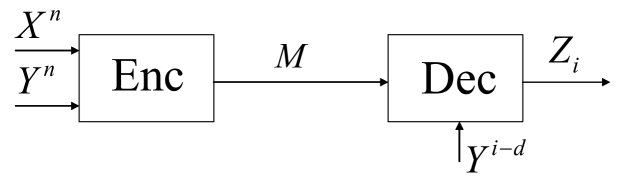
Figure 1: Source coding with delayed side information at the decoder. The side information is fully available at the encoder.

I-A Preliminary Considerations and Related Work

To start, let us first assume that sequences $X^{n}$ and $Y^{n}$ are memoryless sources so that the entries ($X_{i},Y_{i}$) are arbitrarily correlated for a given index $i$ but independent identically distributed (i.i.d.) for different $i=1,...,n.$ To streamline the discussion, the following lemma summarizes the optimal trade-off between rate $R$ and distortion $D$, as measured by a distortion metric $d(x,z)$, for the point-to-point setting of Fig. 1 with memoryless sources. Similar conclusions apply for the more general set-up of Fig. 2.

Lemma 1.

[3, 4, 5] For memoryless source, and zero delay, i.e., $d=0$, the rate-distortion function for the point-to-point system in Fig. 1 is given by the conditional rate-distortion function

$$R(D)=\min_{p(z|x,y):\textrm{ }\textrm{$\mathrm{E}$$[d(X,Z)]\leq D$}}I(X;Z|Y).$$ (1)

This result remains unchanged even if the decoder has access to non-causal side information, i.e., if the reconstruction $Z_{i}$ can be based on the entire sequence $Y^{n}$, rather than only $Y^{i}$. Instead, for strictly positive delay $d>0$, the rate-distortion function is the same as if there was no side information, namely $R(D)=\min_{p(z|x):\textrm{ }\textrm{$\mathrm{E}$$[d(X,Z)]\leq D$}}I(X;Z)$.

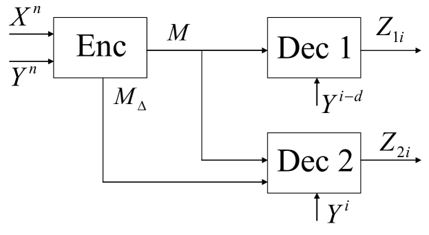
Figure 2: Source coding where side information at the decoder may be delayed and additional information can be delivered when side information is not delayed. The side information is fully available at the encoder.

Similar conclusions can be easily shown to apply also for the more general model of Fig. 2, as it will be discussed in the paper (see Sec. IV). Specifically, if $d>0$ and the sources are memoryless, the rate-distortion function for the system of Fig. 2 with $\Delta R=0$ reduces to the one obtained by Kaspi in [6] for a model in which decoder 1 has no side information, and, for general $\Delta R\geq 0$ , the rate-distortion region coincides with the one obtained in [7] for a model with no side information at decoder 1.

We have seen in Lemma 1 that, for memoryless sources, no advantages can be accrued by leveraging a (strictly) delayed side information, i.e., with $d>0.$ However, this conclusion does not generally hold if the sources have memory. In this context, a number of works have focused on the scenario of Fig. 1 where $X_{i}=Y_{i}$ for $i=1,...n.$ This entails that the decoder observes sequence $X^{n}$ itself, but with a delay of $d$ symbols. This setting is typically referred to as source coding with feedforward, and was introduced in [8]. Reference [1] derived the rate-distortion function for this problem (i.e., Fig. 1 with $X_{i}=Y_{i}$) for ergodic and stationary sources in terms of multi-letter mutual informations. The result was also extended to arbitrary sources using information-spectrum methods. Achievability was obtained via the use of a codebook of codetrees. The function was explicitly evaluated for some special cases in [9, 11] (see also [10]), and [9] proposed an algorithm for its numerical calculation.

The more general case of Fig. 1 with $X_{i}\neq Y_{i}$ was studied in [2] assuming stationary and ergodic sources $X^{n}$ and $Y^{n}$. The rate-distortion function was expressed in terms of multi-letter mutual informations. No specific examples were provided for which the function is explicitly computable. We finally remark that for more complex networks than the ones studied here, strictly delayed side information may be useful even in the presence of memoryless sources. This was illustrated in [12] for a multiple description problem with feedforward.

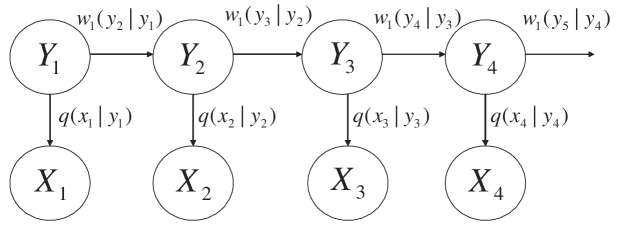
Figure 3: A graphical illustration of the assumed hidden Markov model for the sources.

I-B Contributions

The goal of this work is to characterize the rate-distortion trade-offs for the setting in Fig. 1 and the more general set-up in Fig. 2 for a specific class of sources $X^{n}$ and $Y^{n}$. Specifically, we assume that $Y^{n}$ is a Markov chain, and $X^{n}$ is such that $X_{i}$ is obtained by passing $Y_{i}$ through a channel $q(x|y)$ for $i=1,...,n,$ as illustrated in Fig. 3. The process is thus a hidden Markov model. This model complies with the type of sensor network scenarios described above, where $Y^{n}$ is the physical quantity of interest, modelled as a Markov chain, and $X^{n}$ is a symbol-by-symbol processed version of $Y^{n}.$ The main contributions and the paper organization are as follows. After the description of the system model in Sec. II, for the source statistics described above,

• we derive a single-letter characterization of the minimal rate (bits/source symbol) required for asymptotically lossless compression in the point-to-point model of Fig. 1 for any delay $d\geq 0$ (Sec. III-A). Achievability is based on a novel scheme that consists of simple multiplexing/demultiplexing operations along with standard entropy coding techniques;

• we derive a single-letter characterization of the minimal rate (bits/source symbol) required for lossy compression for the point-to-point model of Fig. 1 and, more generally, for the model of Fig. 2 in which the side information may be delayed, for delays $d=0$ and $d=1$ (Sec. IV);

• we solve a number of specific examples, namely binary-alphabet sources with Hamming distortion and Gaussian sources with minimum mean square error distortion, and present related numerical results (Sec. V).

II System Model

We present the system model for the scenario of Fig. 2. As detailed below, the scenarios of Fig. 1 is obtained as a special case. The system is characterized by a delay $d\geq 0$; finite alphabets $\mathcal{X}$, $\mathcal{Y}$, $\mathcal{Z}_{1}$, $\mathcal{Z}_{2};$ conditional probabilities $w_{1}(a|b)$, with $a,b\in\mathcal{Y},$ and $q(x|y),$ with $x\in\mathcal{X}$ and $y\in\mathcal{Y}$ (i.e., we have $\sum_{a\in\mathcal{Y}}w_{1}(a|b)=1$ and $\sum_{a\in\mathcal{X}}q(a|b)=1$ for all $b\in\mathcal{Y}$); and distortion metrics $d_{j}(x,y,z_{j})$: $\mathcal{X}\times\mathcal{Y}\times\mathcal{Z}_{j}\rightarrow[0,d_{\max}]$, such that $0\leq\mathrm{d}_{j}(x,y,z_{j})\leq\mathrm{d}_{\max}<\infty$ for all $(x,y,z)\in\mathcal{X}\times\mathcal{Y}\times\mathcal{Z}_{j}$ for $j=1,2$. As explained below, the subscript “1” in $w_{1}(a|b)$ indicates that $w_{1}(a|b)$ denotes one-step transition probabilities.

The random process $Y_{i}\in\mathcal{Y}$, $i\in\{...,-1,0,1,...\}$, is a stationary and ergodic Markov chain with transition probability $\Pr[Y_{i}=a|Y_{i-1}=b]=w_{1}(a|b).$ We define the probability $\Pr[Y_{i}=a]\triangleq\pi(a)$ and also the $k$-step transition probability $\Pr[Y_{i}=a_{i}|Y_{i-k}=b]\triangleq w_{k}(a|b),$ which are both independent of $i$ by the stationarity of $Y_{i}$. These quantities can be calculated using standard Markov chain theory from the transition matrix associated with $w_{1}(a|b)$ (see, e.g., [22]). We also set, for notational convenience, $w_{0}(a|b)=\pi(a)$. Sequence $Y^{n}=(Y_{1},...,Y_{n})$ is thus distributed as $p(y^{n})=\pi(y_{1}\mbox{) }\prod\nolimits_{i=2}^{n}w_{1}(y_{i}|y^{i-1})$ for any integer $n>0.$

The random process $X_{i}\in\mathcal{X}$, $i\in\{...,-1,0,1,...\}$ is such that vector $X^{n}=(X_{1},...,X_{n})\in\mathcal{X}^{n}$, for any integer $n>0$, is jointly distributed with $Y^{n}$ so that

$$p(x^{n},y^{n}) =\pi(y_{1}\mbox{)$q(x_{1}|y_{1})$}\prod\limits_{i=2}^{n}p(x_{i},y_{i}|x^{i-1},y^{i-1})$$

$$=\pi(y_{1}\mbox{)$q(x_{1}|y_{1})$}\prod\limits_{i=2}^{n}w_{1}(y_{i}|y^{i-1})q(x_{i}|y_{i}).$$ (2)

In other words, process $X_{i}\in\mathcal{X}$, $i\in\{...,-1,0,1,...\}$ corresponds to a hidden Markov model with underlying Markov process given by $Y^{n}.$

We now define encoder and decoders for the setting of Fig. 2. Specifically, an $(d,n,R,\Delta R,D_{1},D_{2})$ code is defined by: (i) An encoder function

$$\mathrm{f}\text{: }(\mathcal{X}^{n}\times\mathcal{Y}^{n})\rightarrow[1,2^{nR}]\times[1,2^{n\Delta R}],$$ (3)

which maps sequences $X^{n}$ and $Y^{n}$ into messages $M\in[1,2^{nR}]$ and $M_{\Delta}\in[1,2^{n\Delta R}];$ (ii) a sequence of decoding functions for decoder 1

$$\mathrm{g}_{1i}\text{: }[1,2^{nR}]\times\mathcal{Y}^{i-d}\rightarrow\mathcal{Z}_{1},$$ (4)

for $i\in[1,n]$, which, at each time $i,$ map message $M,$ or rate $R$ [bits/source symbol], and the delayed side information $Y^{i-d}$ into the estimate $Z_{1i}$; (iii) a sequence of decoding function for decoder 2

$$\mathrm{g}_{2i}\text{: }[1,2^{nR}]\times[1,2^{n\Delta R}]\times\mathcal{Y}^{i}\rightarrow\mathcal{Z}_{2}$$ (5)

for $i\in[1,n]$, which, at each time $i,$ map messages $M,$ or rate $R,$ and $M_{\Delta},$ of rate or rate $\Delta R,$ and the non-delayed side information $Y^{i}$ into the estimate $Z_{2i}$. In (3)-(5), for $a,b$ integer with $a\leq b$, we have defined $[a,b]$ as the interval $[a,a+1,...,b]$ with $[a,b]=\phi$ if $a>b$. Encoding/decoding functions (3)-(5) must satisfy the distortion constraints

$$\frac{1}{n}\sum\limits_{i=1}^{n}\mathrm{E}[\mathrm{d}_{j}(X_{i},Y_{i},Z_{ji})]\leq D_{j},\text{ for }j=1,2.$$ (6)

Note that these constraints are fairly general in that they allow to impose not only requirements on the lossy reconstruction of $X_{i}$ or $Y_{i}$ (obtained by setting $\mathrm{d}_{j}(x,y,z_{j})$ independent of $y$ or $x,$ respectively), but also on some function of both $X_{i}$ and $Y_{i}$ (by setting $\mathrm{d}_{j}(x,y,z_{j})$ to be dependent on such function of ($x,y$)).

Given a delay $d\geq 0$, for a distortion pair ($D_{1},D_{2}$), we say that rate pair ($R,\Delta R$) is achievable if, for every $\epsilon>0$ and sufficiently large $n$, there exists a $(d,n,R,\Delta R,D_{1}+\epsilon,D_{2}+\epsilon)$ code. We refer to the closure of the set of all achievable rates for a given distortion pair ($D_{1},D_{2}$) and delay $d$ as the rate-distortion region $\mathcal{R}_{d}(D_{1},D_{2})$.

From the general description above for the setting of Fig. 2, the special case of Fig. 1 is produced by neglecting the presence of decoder 2, or equivalently by choosing $D_{2}=\mathrm{d}_{\max}$. In this case, the rate-distortion region $\mathcal{R}_{d}(D_{1},D_{2})$ is fully characterized by a function $R_{d}(D_{1})$ as $\mathcal{R}_{d}(D_{1},\mathrm{d}_{\max})$$=\{(R,\Delta R):\textrm{ $R\geq R_{d}(D_{1}),\mbox{ $\Delta R\geq 0\}$}$}$. Function $R_{d}(D_{1})$ hence characterizes the infimum of rates $R$ for which the pair $(D_{1},\mathrm{d}_{\max})$ is achievable, and is referred to as the rate-distortion function for the setting of Fig. 1. For the special case of the model in Fig. 2 in which $\Delta R=0$, we define the rate-distortion function $R_{d}(D_{1},D_{2})$ in a similar way.

Notation: For $a,b$ integer with $a<b$, we define $x_{a}^{b}=(x_{a},...,x_{b})$; if instead $a<b$ we set $x_{a}^{b}=\emptyset$. We will also write $x_{1}^{b}$ for $x^{b}$ for simplicity of notation. Given a sequence $x^{n}=[x_{1},...,x_{n}]$ and a set $\mathcal{I}=\{i_{1},...,i_{|\mathcal{I}|}\}\subseteq[1,n],$ we define sequence $x^{\mathcal{I}}$ as $x^{\mathcal{I}}=[x_{i_{1}},x_{i_{2}},...,x_{i_{|\mathcal{I}|}}]$ where $i_{1}\leq...\leq i_{|\mathcal{I}|}$. Random variables are denoted with capital letters and corresponding values with lowercase letters. Given random variables, or more generally vectors, $X$ and $Y$ we will use the notation $p_{X}(x)$ or $p(x)$ for $\Pr[X=x]$, and $p_{X|Y}(x|y)$ or $p(x|y)$ for $\Pr[X=x|Y=y]$, where the latter notations are used when the meaning is clear from the context. Given set $\mathcal{X}$, we define $\mathcal{X}^{n}$ as the $n$-fold Cartesian product of $\mathcal{X}$. We denote any function of $\epsilon>0$ that tends to zero as $\epsilon\rightarrow 0$ as $\delta(\epsilon)\rightarrow 0$. When referring to $\epsilon-$typical sequences, we refer to the notion of strong typicality as treated in [14].

III Point-to-Point Model

In this section, we study the point-to-point model in Fig. 1.

III-A Lossless Compression

We start by characterizing the rate-distortion function $R_{d}(D_{1})$ for any delay $d\geq 0$ under the Hamming distortion metric for $D_{1}=0$. The Hamming distortion metric is defined as $\mathrm{d}_{1}(x,y,z_{1})=\mathrm{1}(x\neq z_{1})$, where $\mathrm{1}(a)=1$ if $a$ is true and $\mathrm{1}(a)=0$ otherwise. This implies that the distortion constraint (6) for $j=1$ becomes

$$\frac{1}{n}\sum\limits_{i=1}^{n}\mathrm{E}[1(X_{i}\neq Z_{1i})]=\frac{1}{n}\sum\limits_{i=1}^{n}\Pr[X_{i}\neq Z_{1i}]=0.$$ (7)

In other words, from the definition of achievability given above, we impose that the sequence $X^{n}$ be recovered with vanishingly small average symbol error probability as $n\rightarrow\infty$. We refer to this scenario as asymptotically lossless, or lossless for short.

We have the following characterization of $R_{d}(0)$.

Proposition 1.

For any delay $d\geq 0$, the rate-distortion function for the set-up in Fig. 1 under Hamming distortion at $D_{1}=0$ is given by

$$R_{d}(0)=H(X_{d+1}|X_{2}^{d},Y_{1}),$$ (8)

where the conditional entropy is calculated with respect to the distribution

$$p(y_{1},x_{1}) =\pi(y_{1})q(x_{1}|y_{1})\text{ for }d=0,$$ (9)

$$\text{and }p(y_{1},x_{2},...,x_{d+1}) =\pi(y_{1})\sum_{\begin{subarray}{c}y_{i}\in\mathcal{Y}\\ i\in[2,d+1]\end{subarray}}\prod\limits_{i=2}^{d+1}w_{1}(y_{i}|y_{i-1})q(x_{i}|y_{i})\text{ for }d\geq 1.$$ (10)

The proof of converse of the proposition above is based on an appropriate use of the Fano inequality and is reported in Appendix A. To prove the direct part of the proposition, we propose a simple achievable scheme, which, to the best of the authors’ knowledge, has not appeared before, in Sec. III-B.

Remark 1.

Expression (8) consists of a conditional entropy of $d+1$ random variables, namely $Y_{1}$,$X_{2}$, …, $X_{d+1}$. These variables are distributed as the corresponding entries in the random vectors $X^{n}$ and $Y^{n}$, as per (9)-(10) (cf. (2)). We have therefore used the same notation for the involved random variables as in Sec. II. Proposition 1 provides a “single-letter” characterization of $R_{d}(0)$ for the setting of Fig. 1, since it only involves a finite number of variables. This contrasts with the general characterization for stationary ergodic processes of $R_{d}(D)$ given in [2], which is a “multi-letter” expression, whose computation can generally only attempted numerically using approaches such as the ones proposed in [9]. Note that a multi-letter expression is also given in [11] to characterize $R_{d}(D)$ for i.i.d. sources with negative delays $d<0$. Finally, it should be emphasized that the simple characterization (8) for the scenario of interest here hinges on the assumed statistics of the sources ($X^{n},Y^{n}$).

Remark 2.

By setting $d=0$ in (8) we obtain $R_{0}(0)=H(X_{1}|Y_{1})$. This result generalizes [11, Remark 3, p. 5227] from i.i.d. sources ($X^{n},Y^{n}$) to the hidden Markov model (2) considered here. Note that, for $d=1$, we instead obtain $R_{1}(0)=H(X_{2}|Y_{1}).$ As another notable special case, if side information is absent, or equivalently $d\rightarrow\infty$, in accordance to well-known results, we obtain that $R_{\infty}(0)$ equals the entropy rate (see, e.g., [13])

$$H(\mathcal{X})\triangleq\lim_{n\rightarrow\infty}H(X_{1},..,X_{n}).$$ (11)

In fact, we have

$$R_{\infty}(0)=\lim_{d\rightarrow\infty}H(X_{d+1}|X_{2}^{d},Y_{1})=H(\mathcal{X})$$ (12)

by [13, Theorem 4.5.1].

Remark 3.

Is delayed side information useful (when known also at the encoder)? That this is generally the case follows from the inequality

$$R_{d}(0)=H(X_{d+1}|X_{2}^{d},Y_{1})\leq R_{\infty}(0)=H(\mathcal{X}),$$ (13)

since $R_{\infty}(0)$ is the required rate without side information. This result is proved by the chain of inequalities $H(X_{d+1}|X_{2}^{d},Y_{1})\leq H(X_{d+1}|X_{1}^{d})\leq H(\mathcal{X}),$ where the first inequality follows by the data processing inequality and the second by conditioning reduces entropy. However, inequality (13) may not be strict, and thus side information may not be useful. A first example is the case where $X_{i}$ is an i.i.d. process, which is obtained by making $q(x|y)$ independent of $y$. As another example, consider the setting of source coding with feedforward [8, 1], i.e., $X_{i}=Y_{i}$. In this case, our assumption (2) entails that $X^{n}$ is a Markov chain, and we have $R_{d}(0)=H(X_{d+1}|X_{1}^{d})=H(X_{2}|X_{1})=H(\mathcal{X})$ for $d\geq 1$. Therefore, delayed feedforward (with $d\geq 1)$ is not useful for the lossless compression of Markov chains, as already shown in [8]. This conclusion need not hold for lossy compression (i.e., for $D_{1}>0$) [8] (see also Sec. V-A).

Remark 4.

If $X^{n},Y^{n}$ are general jointly stationary and ergodic processes (and not necessarily stationary ergodic hidden Markov models), one can adapt in a straightforward way the proofs of Appendix A and Sec. III-B, and conclude that the rate distortion function can be written as

$$R_{d}(0)=\lim_{n\rightarrow\infty}\frac{1}{n}H(X^{n}||Y^{n-d}),$$ (14)

where $H(X^{n}||Y^{n-d})$ is the causally conditioned entropy $H(X^{n}||Y^{n-d})=\sum_{i=1}^{n}H(X_{i}|X^{i-1}Y^{i-d})$ (see, e.g., [24]). Comparing (14) with the rate $R_{\infty}(0)=H(\mathcal{X})$ necessary in the absence of any side information, we conclude that the reduction in the compression rate obtained by leveraging delayed side information at the decoder, when side information is known at the encoder, is given for stationary and ergodic processes by

$$R_{\infty}(0)-R_{d}(D)=\lim_{n\rightarrow\infty}\frac{1}{n}I(Y^{n-d}\rightarrow X^{n}).$$ (15)

In (15), we have used the definition of directed mutual information $I(Y^{n-d}\rightarrow X^{n})=H(X^{n})-H(X^{n}||Y^{n-d})$ (see, e.g., [24]). Note that the rate gain (15) complements the results given in [24] on the interpretation of the directed mutual information (see also next remark).

Remark 5.

Consider a variable-length (strictly) lossless source code that operates symbol by symbol such that, for every symbol $i\in[1,n]$, it outputs a string of bits $M_{i}(X^{i},Y^{i-d}),$ which is a function of $X^{i}$ and $Y^{i-d}$. Encoding is constrained so that the code $M_{i}(x^{i},y^{i-d})$ for each ($x^{i},y^{i-d}$) is prefix-free. The decoder, based on delayed side information, can then uniquely decode each codeword $M_{i}(x^{i},y^{i-d})$ as soon as it is received. Following the considerations in [24, Sec. IV], it is easy to verify that rate $R_{d}(0)$ (and, more generally, (14)) is also the infimum of the average rate in bits/source symbol required by such code. Moreover, it is possible to construct universal context-based compression strategies by adapting the approach in [25].

We refer to Sec. V for some examples that further illustrate some implications of Proposition 1.

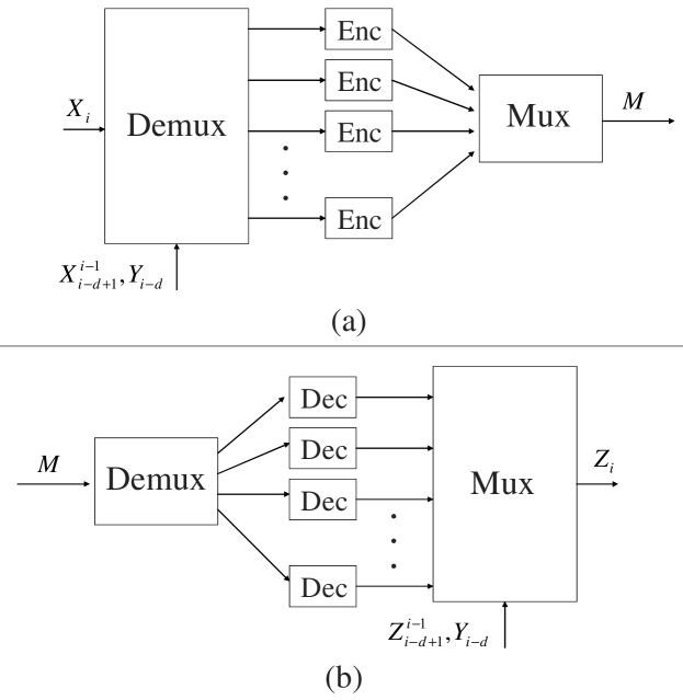
Figure 4: A block diagram for encoder (a) and decoder (b) used in the proof of achievability of Proposition 1.

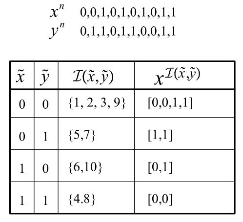
Figure 5: An example that illustrates the operations of the “Demux” block of the encoder used for the achievability proof of Proposition 1, as shown in Fig. 4, for $d=2$ (symbols corresponding to out-of-range indices are set to zero).

III-B Proof of Achievability for Proposition 1

Proof:

(Achievability) Here we propose a coding scheme that achieves rate (8). The basic idea is a non-trivial extension of the approach discussed in [11, Remark 3, p. 5227] and is described as follows. A block diagram is shown in Fig. 4 for encoder (Fig. 4-(a)) and decoder (Fig. 4-(b)).

We first describe the encoder, which is illustrated in Fig. 4-(a). To encode sequences $(x^{n},y^{n})\in(\mathcal{X}^{n}\times\mathcal{Y}^{n}),$ we first partition the interval $[1,n]$ into $|\mathcal{X}|^{d-1}|\mathcal{Y}|$ subintervals, which we denote as $\mathcal{I}(\tilde{x}^{d-1},\tilde{y})\subseteq[1,n]$, for all $\tilde{x}^{d-1}\in\mathcal{X}^{d-1}$ and $\tilde{y}\in\mathcal{Y}$. Every such subinterval $\mathcal{I}(\tilde{x}^{d-1},\tilde{y})$ is defined as

$$\mathcal{I}(\tilde{x}^{d-1},\tilde{y})=\{i\text{: }i\in[1,n]\text{ and }y_{i-d}=\tilde{y},\text{ }x_{i-d+1}^{i-1}=\tilde{x}^{d-1}\}.$$ (16)

In words, the subinterval $\mathcal{I}(\tilde{x}^{d-1},\tilde{y})$ contains all symbol indices $i$ such that the corresponding delayed side information available at the decoder is $y_{i-d}=\tilde{y}$ and the previous $d-1$ samples in $x^{n}$ are $x_{i-d+1}^{i-1}=\tilde{x}^{d-1}$. We refer to the value of the tuple ($y_{i-d},x_{i-d+1}^{i-1}$) as the context of sample $x_{i}$. For the out-of-range indices $i\in[-d+1,0]$, one can assume arbitrary values for $x_{i}\in\mathcal{X}$ and $y_{i}\in\mathcal{Y}$, which are also shared with the decoder once and for all. Note that $\bigcup_{\tilde{x}^{d-1}\in\mathcal{X}^{d-1},\mbox{ }\tilde{y}\in\mathcal{Y}}\mathcal{I}(\tilde{x}^{d-1},\tilde{y})=[1,n]$. Fig. 5 illustrates the definitions at hand for $d=2$.

As a result of the partition described above, the encoder “demultiplexes” sequence $x^{n}$ into $|\mathcal{X}|^{d-1}|\mathcal{Y}|$ sequences $x^{\mathcal{I}(\tilde{x}^{d-1},\tilde{y})}$, one for each possible context ($\tilde{x}^{d-1},\tilde{y})\in\mathcal{X}^{d-1}\mathcal{\times Y}$. This demultiplexing operation, which is controlled by the previous values of source and side information, is performed in Fig. 4-(a) by the block labelled as “Demux”, and an example of its operation is shown in Fig. 5. By the ergodicity of process $X_{i}$ and $Y_{i}$, for every $\epsilon>0$ and all sufficiently large $n$, the length of any sequence $x^{\mathcal{I}(\tilde{x}^{d-1},\tilde{y})}$ is guaranteed to be less than $np_{Y_{1}X_{2},...,X_{d}}(\tilde{y},\tilde{x}^{d-1})+\epsilon$ symbols with probability arbitrarily close to one. This because the length $|\mathcal{I}(\tilde{x}^{d-1},\tilde{y})|$ of the sequence $x^{\mathcal{I}(\tilde{x}^{d-1},\tilde{y})}$ equals the number of occurrences of the context ($y_{i-d}=\tilde{y},\text{ }x_{i-d+1}^{i-1}=\tilde{x}^{d-1}$) and by Birkhoff’s ergodic theorem (see [13, Sec. 16.8]). In particular, for any $\epsilon>0$ we can find an $n$ such that

$$\Pr[\mathcal{E}_{1}(\tilde{y},\tilde{x}^{d-1})]\leq\frac{\epsilon}{2|\mathcal{X}|^{d-1}|\mathcal{Y}|},$$ (17)

where we have defined the “error” event

$$\mathcal{E}_{1}(\tilde{y},\tilde{x}^{d-1})=\{|\mathcal{I}(\tilde{x}^{d-1},\tilde{y})|>np_{Y_{1}X_{2},...,X_{d}}(\tilde{y},\tilde{x}^{d-1})+\epsilon\}.$$ (18)

Each sequence $x^{\mathcal{I}(\tilde{x}^{d-1},\tilde{y})}$ is encoded by a separate encoder, labelled as “Enc” in Fig. 4-(a). In case the cardinality $|\mathcal{I}(\tilde{x}^{d-1},\tilde{y})|$ does not exceed $np_{Y_{1}X_{2},...,X_{d}}(\tilde{y},\tilde{x}^{d-1})+\epsilon$ (i.e., the “error” event $\mathcal{E}_{1}(\tilde{y},\tilde{x}^{d-1})$ does not occur), the encoder compresses sequence $x^{\mathcal{I}(\tilde{x}^{d-1},\tilde{y})}$ using an entropy encoder, as explained below. If the cardinality condition is instead not satisfied (i.e., $\mathcal{E}_{1}(\tilde{y},\tilde{x}^{d-1})$ is realized), then an arbitrary bit sequence of length $L_{\epsilon}(\tilde{y},\tilde{x}^{d-1})$, to be specified below, is selected by the encoder “Enc”.

The entropy encoder can be implemented in different ways, e.g., using typicality or Huffman coding (see, e.g., [13]). Here we consider a typicality-based encoder. Note that the entries $X_{i}$ of each sequence $X^{\mathcal{I}(\tilde{x}^{d-1},\tilde{y})}$ are i.i.d. with distribution $p_{X_{d+1}|Y_{1}X_{2},...,X_{d}}(\cdot|\tilde{y},\tilde{x}^{d-1})$, since conditioning on the context $\{y_{i-d}=\tilde{y},\text{ }x_{i-d+1}^{i-1}=\tilde{x}^{d-1}\}$ makes the random variables $X_{i}$ independent. As it is standard practice, the entropy encoder assigns a distinct label to all $\epsilon$-typical sequences $\mathcal{T}_{\epsilon}(p_{X_{d+1}|Y_{1}X_{2},...,X_{d}}(\cdot|\tilde{y},\tilde{x}^{d-1}))$ with respect to such distribution, and an arbitrary label to non-typical sequences. From the Asymptotic Equipartion Property (AEP), we can choose $n$ sufficiently large so that (see, e.g., [14])

$$\Pr[\mathcal{E}_{2}(\tilde{y},\tilde{x}^{d-1})]\leq\frac{\epsilon}{2|\mathcal{X}|^{d-1}|\mathcal{Y}|},$$ (19)

where we have defined the “error” event

$$\mathcal{E}_{2}(\tilde{y},\tilde{x}^{d-1})=\{X^{\mathcal{I}(\tilde{x}^{d-1},\tilde{y})}\notin\mathcal{T}_{\epsilon}(p_{X_{d+1}|Y_{1}X_{2},...,X_{d}}(\cdot|\tilde{y},\tilde{x}^{d-1}))\}.$$ (20)

Moreover, by the AEP, a rate in bits per source symbol of $H(X_{d+1}|X_{2}^{d}=\tilde{x}^{d-1},Y_{1}=\tilde{y})+\epsilon$ is sufficient for the entropy encoder to label all $\epsilon$-typical sequences.

From the discussion above, it follows that the proposed scheme encodes each sequence $x^{\mathcal{I}(\tilde{x}^{d-1},\tilde{y})}$ with $L_{\epsilon}(\tilde{y},\tilde{x}^{d-1})=np_{Y_{1}X_{2},...,X_{d}}(\tilde{y},\tilde{x}^{d-1})H(X_{d+1}|X_{2}^{d}=\tilde{x}^{d-1},Y_{1}=\tilde{y})+n\delta(\epsilon)$ bits. By concatenating the descriptions of all the $|\mathcal{X}|^{d-1}|\mathcal{Y}|$ sequences $x^{\mathcal{I}(\tilde{x}^{d-1},\tilde{y}_{1})}$, we thus obtain that the overall rate $R$ of message $M$ for the scheme at hand is $H(X_{d+1}|X_{2}^{d-1},Y_{1})+\delta(\epsilon)$. The concatenation of the labels output by each entropy encoder is represented in Fig. 4-(a) by the block “Mux”. We emphasize that encoder and decoder agree a priori on the order in which the descriptions of the different subsequences are concatenated. For instance, with reference to the example in Fig. 5 (with $d=2$), message $M$ can contain first the description of the sequence corresponding to $(\tilde{x},\tilde{y})=(0,0)$, then $(\tilde{x},\tilde{y})=(0,1)$, etc.

We now describe the decoder, which is illustrated in Fig. 4-(b). By undoing the multiplexing operation just described, the decoder, from the message $M$, can recover the individual sequences $x^{\mathcal{I}(\tilde{x}^{d-1},\tilde{y})}$ through a simple demultiplexing operation for all contexts $(\tilde{x}^{d-1},\tilde{y})\in\mathcal{X}^{d-1}\times\mathcal{Y}$. This operation is represented by block “Demux” in Fig. 4-(b). To be precise, this demultiplexing is possible, unless the encoding “error” event

$$\mathcal{E}=\bigcup_{\tilde{x}^{d-1}\in\mathcal{X}^{d-1},\mbox{ }\tilde{y}\in\mathcal{Y}}\{\mathcal{E}_{1}(\tilde{y},\tilde{x}^{d-1})\cup\mathcal{E}_{2}(\tilde{y},\tilde{x}^{d-1})\}$$ (21)

takes place. In fact, occurrence of the “error” event $\mathcal{E}$ implies that some of the sequences $x^{\mathcal{I}(\tilde{x}^{d-1},\tilde{y})}$ was not correctly encoded and hence cannot be recovered at the decoder. The effect of such errors will be accounted for below.

Assume now that no error has taken place in the encoding. While the individual sequences $x^{\mathcal{I}(\tilde{x}^{d-1},\tilde{y})}$ can be recovered through the discussed demultiplexing operation, this does not imply that the decoder is also able to recover the original sequence $x^{n}$. In fact, that decoder does not know a priori the partition $\{\mathcal{I}(\tilde{x}^{d-1},\tilde{y})$: $\tilde{x}^{d-1}\in\mathcal{X}^{d-1}$ and $\tilde{y}\in\mathcal{Y}\}$ of the interval $[1,n]$ and thus cannot reorder the elements of sequences $x^{\mathcal{I}(\tilde{x}^{d-1},\tilde{y})}$ to produce $x^{n}$. Recall, moreover, that such re-ordering operation should be done in a causal fashion following the decoding rule (4).

We now argue that the re-ordering mentioned above is in fact possible using a decoding rule that complies with (4) via a multiplexing block controlled by the previous estimates of the source samples (block “Mux” in Fig. 4-(b)). In fact, note that at time $i$, the decoder knows $Y_{i-d}$ and the previously decoded $X^{i-1}$ and can thus identify the subinterval $\mathcal{I}(\tilde{x}^{d-1},\tilde{y})$ to which the current symbol $X_{i}$ belongs. This symbol can be then immediately read as the next yet-to-be-read symbol from the corresponding sequence $x^{\mathcal{I}(\tilde{x}^{d-1},\tilde{y})}$. Note that for the first $d$ symbols, the decoder uses the values for $x_{i}$ and $y_{i}$ at the out-of-range indices $i$ that were agreed upon with the encoder (see above). In conclusion, we remark that the scheme described above, by choosing $\epsilon$ small enough and $n$ large enough, is able to satisfy the constraint (7) to any desired accuracy. We also note that the controlled multiplexing/demultiplexing operation used in the proof is reminiscent of the scheme proposed in [26] for transmission on fading channels with side information at the transmitter and receiver.

We finally need to study the effect of errors. Given the choices made above, we have that the probability of an encoding error is

$$\Pr[\mathcal{E}] \leq\sum_{\tilde{x}^{d-1}\in\mathcal{X}^{d-1},\mbox{ }\tilde{y}\in\mathcal{Y}}\Pr[\mathcal{E}_{1}(\tilde{y},\tilde{x}^{d-1})]+\Pr[\mathcal{E}_{2}(\tilde{y},\tilde{x}^{d-1})]\leq\epsilon,$$ (22)

where the first inequality follows from the union bound and the second from (17) and (19). This implies that the distortion in (7) is upper bounded by $\epsilon$ as desired. In fact, from the definition of encoder and decoder given above, we can conclude that $\Pr[X^{n}\neq Z_{1}^{n}]=\Pr[\mathcal{E}]\leq\epsilon$, where we recall that $Z_{1}^{n}$ is the sequence reconstructed at the decoder. Moreover, the following inequality holds in general

$$\Pr[X^{n}\neq Z_{1}^{n}]\geq\frac{1}{n}\sum\limits_{i=1}^{n}\Pr[X_{i}\neq Z_{1i}].$$ (23)

Therefore, we have $\frac{1}{n}{\textstyle{\textstyle{\displaystyle\sum\limits_{i=1}^{n}}}}\Pr[X_{i}\neq Z_{1i}]\leq\epsilon$, which concludes the proof. ∎

Remark 6.

An alternative proof of achievability can be given by using the idea of codetrees and extending the notions of typicality introduced in [1]. The proof discussed above is based on a conceptually and algorithmically simpler approach, albeit its applicability is limited to lossless compression (see next subsection).

Remark 7.

From the inequality (23), it follows that the optimality of the scheme above can be proved also under the more stringent block error probability constraint (see also [14, Sec. 3.6.4]).

III-C Lossy Compression

Here, we obtain a characterization of the rate-distortion function $R_{d}(D_{1})$, for $d=0$ and $d=1$. The proof follows as a special case of that of Proposition 4 to be discussed in the next section, and is based on similar arguments as for Proposition 1.

Proposition 2.

For any delay $d\geq 0$ and distortion $D_{1}$, the following rate is achievable for the setting of Fig. 1

$$R_{d}^{(a)}(D_{1})=\min I(XY;Z_{1}|Y_{d}),$$ (24)

with mutual informations evaluated with respect to the joint distribution

$$p(x,y,y_{d},z_{1})=\pi(y_{d})w_{d}(y|y_{d})q(x|y)p(z_{1}|x,y,y_{d}),$$ (25)

and where minimization is done over all conditional distributions $p(z_{1}|x,y,y_{d})$ such that

$$\mathrm{E}[d_{1}(X,Y,Z_{1})]\leq D_{1}.$$ (26)

Moreover, rate (24)-(26) is the rate-distortion function, i.e., $R_{d}^{(a)}(D_{1})=R_{d}(D_{1})$, for $d=0$ and $d=1$.

Remark 8.

The optimality of the conditional codebook strategy for lossless compression shown in Proposition 1 hinges on the following fact: conditioned on the context ($Y_{i-d},X_{i-d+1},$ $\text{\ldots},X_{i-1}$), the samples $X_{i}$ are independent of the past samples $X^{i-1}$ by the hidden Markov model assumption. Recall that the fact that the decoder has available the past source samples ($X_{i-d+1},$$\text{\ldots},X_{i-1}$) since its estimates are correct with high probability. Due to this independence property, and to the availability of the side information also at the encoder, the latter need not use “multi-letter” compression codes and can instead use simple “single-letter” entropy codes conditioned on the values of ($Y_{i-d},X_{i-d+1},$$\text{\ldots},X_{i-1}$) without loss of optimality. In the lossy case considered in Proposition 2, instead, even for the point-to-point model, the independence condition discussed above does not hold for delays $d$ strictly larger than 1. In fact, at each time $i$, the decoder has available the delayed side information $Y^{i-d}$ only, conditioned on which the source samples $X_{i}$ are not independent of the past samples $X^{i-1}$. But, for $d=1$, the independence condition at hand does apply and thus the optimality of “single-letter” codes can be proved as done in Proposition 2.

IV When the Side Information May Be Delayed

In this section, we consider the problem of lossy compression for the set-up of Fig. 2. Note that the asymptotically lossless case follows from Proposition 1, since, in order to guarantee lossless reconstruction also at the decoder with delayed side information, rate $R$ must satisfy the conditions in Proposition 1. Here, we obtain an achievable rate region $\mathcal{R}_{d}^{(a)}(D_{1},D_{2})\mathcal{\subseteq R}_{d}(D_{1},D_{2})$ for all delays $d\geq 0$ for the model in Fig. 2, and show that such region coincides with the rate-distortion region, i.e., $\mathcal{R}_{d}^{(a)}(D_{1},D_{2})\mathcal{=R}_{d}(D_{1},D_{2})$, for $d=0$ and $d=1$.

To streamline the discussion, we start by consider the special case where $\Delta R=0$ and obtain a characterization of the rate-distortion function $R_{d}(D_{1},D_{2})$ for $d=0$ and $d=1$.

Proposition 3.

For any delay $d\geq 0$ and distortion pair $(D_{1},D_{2})$, the following rate is achievable for the set-up of Fig. 2 with $\Delta R=0$

$$R_{d}^{(a)}(D_{1},D_{2}) =\min I(XY;Z_{1}|Y_{d})+I(X;Z_{2}|YY_{d}Z_{1})$$ (27)

$$=\min I(Y;Z_{1}|Y_{d})+I(X;Z_{1}Z_{2}|YY_{d}),$$ (28)

with mutual informations evaluated with respect to the joint distribution

$$p(x,y,y_{d},z_{1},z_{2})=\pi(y_{d})w_{d}(y|y_{d})q(x|y)p(z_{1},z_{2}|x,y,y_{d}),$$ (29)

and where minimization is done over all conditional distributions $p(z_{1},z_{2}|x,y,y_{d})$ such that

$$\mathrm{E}[d_{j}(X,Y,Z_{j})]\leq D_{j}\text{, for }j=1,2.$$ (30)

Moreover, rate (27)-(28) is the rate-distortion function, i.e., $R_{d}^{(a)}(D_{1},D_{2})=R_{d}(D_{1},D_{2})$, for $d=0$ and $d=1$.

Remark 9.

Rate (27) can be easily interpreted in terms of achievability. To this end, we remark that variable $Y_{d}$ plays the role of the delayed side information $Y^{i-d}$ at decoder 1. The coding scheme achieving rate (27) operates in two successive phases. In the first phase, the encoder encodes the reconstruction sequence $Z_{1}^{n}$ for decoder 1. Since decoder 1 has available delayed side information, using a strategy similar to the one discussed in Sec. III-B, this operation requires $I(XY;Z_{1}|Y_{d})$ bits per source sample, as further detailed in Sec. IV-A. Note that decoder 2 is able to recover $Z_{1}^{n}$ as well, since decoder 2 has available side information $Y^{i}$, and thus also the delayed side information $Y^{i-d}$. In the second phase, the reconstruction sequence $Z_{2}^{n}$ for decoder 2 is encoded. Given the side information available at decoder 2, this operation requires rate $I(X;Z_{2}|YY_{d}Z_{1})$, using again an approach similar to the one discussed in Sec. III-B. The converse proof is in Appendix B.

Remark 10.

For memoryless sources $X^{n}$ and $Y^{n}$, obtained by setting the transition probability $w_{1}(y_{i}|y^{i-1})$ to be independent of $y^{i-1}$, it can be seen that the achievable rate (27)-(28) is the rate-distortion function for the scenario of Fig. 2 with $\Delta R=0$ for all delays $d\geq 0$. This observation extends Lemma 1 to the more general set-up of Fig. 2 with $\Delta R=0$. To see this, note that for $d\geq 1$, rate (27)-(28) is given by

$$R_{d}^{(a)}(D_{1},D_{2})=\min I(XY;Z_{1})+I(X;Z_{2}|YZ_{1}),$$ (31)

with mutual informations evaluated with respect to the joint distribution

$$p(x,y,y_{d},z_{1},z_{2})=\pi(y)q(x|y)p(z_{1},z_{2}|x,y),$$ (32)

and where minimization is done over all conditional distributions $p(z_{1},z_{2}|x,y,y_{d})$ such that the distortion constraints (30) are satisfied. Rate (31) recovers the rate-distortion function derived by [6] for the case where decoder 1 has no side information. Therefore, rate (31) is achievable even without any state information at decoder 1. We then conclude that delayed side information is not useful for memoryless sources. Note also that [6] assumes non-causal availability of the side information at decoder 2. The equality of the rate derived in [6] and the one in Proposition 3 thus demonstrates that causal and non-causal side information lead to the same performance in terms of rate-distortion function.

Remark 11.

While (27) is easier to interpret in terms of achievability as done in Remark 9, the equivalent expression (28) highlights the rate loss due to the possible delay of the side information. In fact, the mutual information $I(X;Z_{1}Z_{2}|YY_{d})$ accounts for the rate that would be needed to convey both $Z_{1}^{n}$ and $Z_{2}^{n}$ only to decoder 2, which has non-delayed side information. Therefore, the additional term $I(Y;Z_{1}|Y_{d})$ can be interpreted as the extra rate that needs to be expended to enable transmission of $Z_{1}^{n}$ also to decoder 1, which has delayed side information.

We now consider the general model in Fig. 2.

Proposition 4.

For any delay $d\geq 0$ and any distortion pair ($D_{1},D_{2}$), define $\mathcal{R}_{d}^{(a)}(D_{1},D_{2})$ as the union of all rate pairs ($R,\Delta R$) that satisfy

$$R \geq I(Y;Z_{1}|Y_{d})+I(X;Z_{1}U|YY_{d})$$ (33)

$$R+\Delta R \geq I(Y;Z_{1}|Y_{d})+I(X;Z_{1}Z_{2}U|YY_{d})$$ (34)

for some joint distribution

$$p(x,y,y_{d},u,z_{1},z_{2})=\pi(y_{d})w_{d}(y|y_{d})q(x|y)p(z_{1},z_{2},u|x,y,y_{d})$$ (35)

where minimization is done over all conditional distributions $p(z_{1},z_{2},u|x,y,y_{d})$ such that

$$\mathrm{E}[d_{j}(X,Y,Z_{j})]\leq D_{j}\text{, for }j=1,2.$$ (36)

We have that

$$\mathcal{R}_{d}^{(a)}(D_{1},D_{2})\mathcal{\subseteq R}_{d}(D_{1},D_{2})$$ (37)

for any $d\geq 0$. Moreover, equation (37) holds with equality, and thus $\mathcal{R}_{d}^{(a)}(D_{1},D_{2})$ is the rate-distortion region, for $d=0$ and $d=1$.

Remark 12.

Let us interpret the rate region $\mathcal{R}_{d}^{(a)}(D_{1},D_{2})$ in terms of achievability. First, from Remark 9, we observe that (33) is the rate necessary to convey $Z_{1}^{n}$ to both decoder 1 and decoder 2, and an auxiliary codeword $U^{n}$ only to decoder 2. This auxiliary codeword $U^{n}$ carries information to decoder 2 that is then refined via message $M_{\Delta}.$ In particular, rewriting (34) as $R+\Delta R\geq I(Y;Z_{1}|Y_{d})+I(X;Z_{1}U|YY_{d})+I(X;Z_{2}|YY_{d}UZ_{1})$, by comparison with (33), we see that the extra rate $I(X;Z_{2}|YY_{d}UZ_{1})$ is needed to transmit sequence $Z_{2}^{n}$ to decoder 2, thus refining the information available therein due to message $M$.

Remark 13.

The considerations in Remark 10 can be also easily extended to the scenario of Proposition 4 with $\Delta R\geq 0$.

IV-A Proof of Achievability of Proposition 3 and Proposition 4

Proof:

(Achievability) We first prove achievability of rate (27) in Proposition 3. The proof extends the ideas discussed in Sec. III-B, to which we refer for details. In particular, here we do not detail the calculations of the encoding “error” events and distortion levels, as they follow in the same way as in Sec. III-B. To encode sequence ($x^{n},y^{n}$), the encoder partitions the interval $[1,n]$ into $|\mathcal{Y}|$ subintervals, namely $\mathcal{I}(\tilde{y})$ for each $\tilde{y}\in\mathcal{Y}$, so that (cf. (16))

$$\mathcal{I}(\tilde{y})=\{i\text{: }i\in[1,n]\text{ and }y_{i-d}=\tilde{y}\}.$$ (38)

Similar to Sec. III-B, a different compression codebook is used for each such interval $\mathcal{I}(\tilde{y})$, and thus for each pair of “demultiplexed” subsequences $(x^{\mathcal{I}(\tilde{y})},y^{\mathcal{I}(\tilde{y})})$. The compression of each pair of sequences $(x^{\mathcal{I}(\tilde{y})},y^{\mathcal{I}(\tilde{y})})$ is based on a test channel $p(z_{1}|x,y,\tilde{y}).$ Specifically, the corresponding codewords $Z_{1}^{n}$ are generated i.i.d. according to the marginal distribution $\sum_{(x,y)\in\mathcal{Y}}p(z_{1}|x,y,\tilde{y})$ $w_{1}(y|\tilde{y})q(x|y)$ and compression is done based on standard joint typicality arguments. By the covering lemma [14], compression of sequences $(X^{\mathcal{I}(\tilde{y})},Y^{\mathcal{I}(\tilde{y})})$ into the corresponding reconstruction sequence $Z_{1}^{\mathcal{I}(\tilde{y})}$ requires rate $I(XY;Z_{1}|\tilde{Y}=\tilde{y})+\epsilon$ bits per source symbol in each interval $\mathcal{I}(\tilde{y})$, and thus an overall rate $I(XY;Z_{1}|\tilde{Y})+\epsilon$ following the same considerations as in Sec. III-B. In particular, the encoder multiplexes the compression indices corresponding to the $|\mathcal{Y}|$ intervals $\mathcal{I}(\tilde{y})$ to produce message $M$. Therefore, the latter only carries information about the individual sequences $Z_{1}^{\mathcal{I}(\tilde{y})},$ but not about the ordering of each entry within the overall sequence $Z_{1}^{n}$.

Based on the sequence $z_{1}^{n}$ produced in the first encoding phase described above, the encoder then performs also a finer partition of the interval $[1,n]$ into $|\mathcal{Y}|^{2}|\mathcal{Z}_{1}|$ intervals $\mathcal{I}(\tilde{y},y,z),$ with $\tilde{y}\in\mathcal{Y},\mbox{ }y\in\mathcal{Y},\mbox{ and }z\in\mathcal{Z}$, so that

$$\mathcal{I}(\tilde{y},y,z)=\{i\text{: }i\in[1,n]\text{ and }y_{i-d}=\tilde{y},\mbox{ }y_{i}=y,\mbox{\mbox{ }and }z_{i}=z\}.$$ (39)

Compression of sequence $x^{I(\tilde{y},y,z)}$ into the corresponding reconstruction $Z_{2}^{\mathcal{I}(\tilde{y},y,z)}$ is carried out according to test channel $p(z_{2}|x,y,\tilde{y},z)$ as per the discussion above, requiring an overall rate of $I(X;Z_{2}|Y\tilde{Y}Z_{1})+\epsilon.$ The compression indices for all sets $\mathcal{I}(\tilde{y},y,z)$ are concatenated in message $M$ following the compression indices obtained from the sets $\mathcal{I}(\tilde{y})$.

Upon reception of message $M$, decoder 1 and 2 can both recover the sequences $Z_{1}^{\mathcal{I}(\tilde{y})}$ and $Z_{2}^{\mathcal{I}(\tilde{y},y,z)}$ for all $\tilde{y}\in\mathcal{Y},$ $y\in\mathcal{Y}$ and $z\in\mathcal{Z}$ via simple demultiplexing. Moreover, following the same reasoning as in Sec. III-B, decoder 1 can reconstruct sequence $Z_{1}^{n}$ in the correct order in a causal fashion, using a decoder (4), which depends on message and delayed side information, since the value of $Z_{1i}$ can be obtained from sequences $Z_{1}^{\mathcal{I}(\tilde{y})}$ by knowing the value of $Y_{i-d}.$ Similarly, decoder 2 can reorder sequence $Z_{2}^{n}$ in a causal fashion using a decoder of the form (5). This concludes the proof of achievability for Proposition 3. ∎

We now turning to the proof of achievability Proposition 4. For a fixed distribution (35), we need to prove that the rate region in Fig. 6 is achievable. To do this, it is enough, by standard time-sharing arguments, to prove that corner points A and B are achievable. Corner point B corresponds to rate pair $R=I(Y;Z_{1}|Y_{d})+I(X;Z_{1}Z_{2}U|YY_{d})$ and $\Delta R=0$. But achievability of this region follows immediately from Proposition 3 by setting $U=(UZ_{2})$ in (27). Instead, corner point A corresponds to the rate pair

$$R =I(Y;Z_{1}|Y_{d})+I(X;Z_{1}U|YY_{d})$$ (40)

$$\text{and }\Delta R =I(X;Z_{2}|UYY_{d}Z_{1}).$$ (41)

This rate pair can be achieved by using a strategy similar to the one discussed above. In this strategy, when encoding the message $M_{\Delta}$, which is received only at decoder 2, the encoder leverages the fact that the latter knows $Y_{i},Y_{i-d},U_{i}$ and $Z_{1i}$, by appropriately partitioning the interval $[1,n]$ and using different test channels in each subinterval. ∎

V Examples

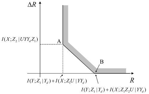
Figure 6: Achievable rate region used in the proof of Proposition 4.

In this section, we consider two specific examples relative to the scenario in Fig. 1. The first example consists of binary-alphabet sources, while the second applies the results derived above to (continuous-alphabet) Gaussian sources. We focus on a distortion metric of the form $\mathrm{d}_{1}(x,y,z_{1})=\mathrm{d}_{1}(x,z_{1})$ that does not depend on $y.$ In other words, the decoder is interested in reconstructing $X^{n}$ within some distortion $D_{1}$. We note that, under this assumption, the rate (2) equals the simpler expression

$$R_{d}^{(a)}(D_{1})=\min I(X;Z_{1}|Y_{d}),$$ (42)

with mutual informations evaluated with respect to the joint distribution

$$p(x,y_{d},z_{1})=\pi(y_{d})\left(\mbox{$\sum_{y\in\mathcal{Y}}$}w_{d}(y|y_{d})q(x|y)\right)p(z_{1}|x,y_{d}),$$ (43)

where minimization is done over all distributions $p(z_{1}|x,y_{d})$ such that $\mathrm{E}[\mathrm{d}_{1}(X,Z_{1})]\leq D_{1}.$ Note that this simplification is without loss of optimality because the distortion constraint does not depend on the correlation between $Z_{1}$ and $Y.$ Therefore, we can impose the Markov condition $Z_{1}-XY_{d}-Y$ as in (42) without changing the distortion, while reducing the mutual information in (24).

V-A Binary Hidden Markov Model

In the first example, we assume that $Y_{i}$ is a binary Markov chain with symmetric transition probabilities $w_{1}(1|0)=w_{1}(0|1)\triangleq\varepsilon$. Therefore, we have $\pi(1)=1/2$ and $k$-step transition probabilities $w_{k}(1|0)=w_{k}(0|1)\triangleq\varepsilon^{(k)}$, which can be obtained recursively as $\varepsilon^{(1)}=\varepsilon$ and $\varepsilon^{(k)}=2\varepsilon^{(k-1)}(1-\varepsilon^{(k-1)})$ for $k\geq 2$. Note that this is a logistic map such that $\varepsilon^{(k)}\rightarrow 1/2$ for large $k$. We also set $\varepsilon^{(0)}=0$, consistently with the convention adopted in the rest of the paper. Finally, we assume that

$$X_{i}=Y_{i}\oplus N_{i},$$ (44)

with “$\oplus$” being the modulo-2 sum and $N_{i}$ being i.i.d. binary variables, independent of $Y^{n}$, with $p_{N_{i}}(1)\triangleq q$, $q\leq 1/2$. We adopt the Hamming distortion $d_{1}(x,z_{1})=x\oplus z_{1}$.

We start by showing in Fig. 7 the rate $R_{d}(0)$ obtained from Proposition 1 corresponding to zero distortion ($D_{1}=0$) versus the delay $d$ for different values of $\varepsilon$ and for $q=0.1$. Note that the value of $\varepsilon$ measure the “memory” of the process $Y_{i}$: For $\varepsilon$ small, the process tends to keep its current value, while for $\varepsilon=1/2$, the values of $Y_{i}$ are i.i.d.. For $d=0$, we have $R_{0}(0)=H(X_{1}|Y_{1})=H_{b}(q)=0.589$, irrespective of the value of $\varepsilon$, where we have defined the binary entropy function $H_{b}(a)=-a\log_{2}a-(1-a)\log_{2}(1-a)$. Instead, for $d$ increasingly large, the rate $R_{d}(0)$ tends to the entropy rate $R_{\infty}(0)=H(\mathcal{X})$. This can be calculated numerically to arbitrary precision following [13, Sec. 4.5]. Note that a larger memory, i.e., a smaller $\varepsilon$ leads to smaller required rate $R_{d}(0)$ for all values of $d$.

Fig. 8 shows the rate $R_{d}(0)$ for $\varepsilon=0.1$ versus $q$ for different values of $d$. For reference, we also show the performance with no side information, i.e., $R_{\infty}(0)=H(\mathcal{X})$. For $q=1/2$, the source $X^{n}$ is i.i.d. and delayed side information is useless in the sense that $R_{d}(0)=R_{\infty}(0)=H(X_{1})=1$ (Remark 3). Moreover, for $q=0$, we have $X_{i}=Y_{i}$, so that $X_{i}$ is a Markov chain and the problem becomes one of lossless source coding with feedforward. From Remark 3, we know that delayed side information is useless also in this case, as $R_{d}(0)=R_{\infty}(0)=H(\mathcal{X})=H_{b}(\varepsilon)=0.469$. For intermediate values of $q$, side information is generally useful, unless the delay $d$ is too large.

We now turn to the case where the distortion $D_{1}$ is generally non-zero. To this end, we evaluate the achievable rate (42) in Appendix C obtaining

$$R_{d}^{(a)}(D_{1})=H_{b}(\varepsilon^{(d)}*q)-H_{b}(D_{1})$$ (45)

for

$$0\leq D_{1}\leq\min\{\varepsilon^{(d)}*q,1-\varepsilon^{(d)}*q\},$$ (46)

and $R_{d}^{(a)}(D_{1})=0$ otherwise. In (45)-(46) we have defined $p*q\triangleq p(1-q)+(1-p)q$. Recall that rate $R_{d}^{(a)}(D_{1})$ has been proved to coincide with the rate-distortion function $R_{d}(D_{1})$ only for $d=0\mbox{ and }d=1$ (Corollary 2).

As a final remark, we use the result derived above to discuss the advantages of delayed side information. To this end, set $q=0$ so that $X_{i}=Y_{i}$ and the problem becomes one of source coding with feedforward. For $d=1$, result (45)-(46) recovers the calculation in [8, Example 2] (see also [9]), which states that the rate-distortion function for the Markov source $X^{n}$ at hand with feedforward ($d=1$) is

$$R_{1}(D)=H_{b}(\mathcal{\varepsilon})-H_{b}(D_{1})$$ (47)

for $D_{1}\leq\min(\varepsilon,1-\varepsilon)$ and $R_{1}(D_{1})=0$ otherwise. From [19] (see also [21]), it is known that the rate-distortion function of a Markov source $X^{n}$ without feedforward, i.e., $R_{\infty}(D_{1})$, is equal to (47) only for $D_{1}$ smaller than a critical value, but is otherwise larger. This demonstrates that feedforward, unlike in the lossless setting discussed above, can be useful in the lossy case for distortion levels $D_{1}$ sufficiently large, as first discussed in [8].

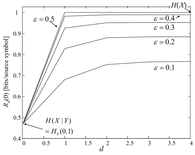
Figure 7: Minimum required rate $R_{d}(0)$ for lossless reconstruction for the set-up of Fig. 1 with binary sources versus delay $d$ ($q=0.1$).

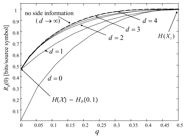
Figure 8: Minimum required rate $R_{d}(0)$ for lossless reconstruction for the set-up of Fig. 1 with binary sources versus parameter $q$ ($\varepsilon=0.1$).

V-B Hidden Gauss-Markov Model

We now assume that $Y^{n}$ is a Gauss-Markov process with zero-mean, power $E[Y_{i}^{2}]=1$ and correlation $\mathrm{E}[Y_{i}Y_{i+1}]=\rho$ (so that $\mathrm{E}[Y_{i}Y_{i+d}]=\rho^{d}$). Moreover, $X_{i}$ is related to $Y_{i}$ as

$$X_{i}=Y_{i}+N_{i},$$ (48)

where samples $N_{i}$ are i.i.d. zero-mean Gaussian with variance $\sigma_{N}^{2}$ and independent of $Y^{n}$. We concentrate on the mean square error distortion metric $\mathrm{d}_{1}(x,z_{1})=(x-z_{1})^{2}$. Using standard arguments, we can apply the achievable rate (42) to the setting at hand, although the result was derived for discrete alphabet (see [14, Ch. 3.8]). By doing so, as shown in Appendix D, we get that the following rate is achievable for $d\geq 0$

$$R_{d}^{(a)}(D_{1})=\frac{1}{2}\log_{2}\left(\frac{1-\rho^{2d}+\sigma_{N}^{2}}{D_{1}}\right)$$ (49)

if $0\leq D_{1}\leq 1-\rho^{2d}+\sigma_{N}^{2}$ and $R_{d}^{(a)}(D_{1})=0$ otherwise. As also discussed above, this rate coincides with the rate-distortion function for $d=0$ and $d=1$.

Similar to the discussion in the previous section for a binary hidden Markov model, we remark that for $\sigma_{N}^{2}=0$, the problem becomes one of lossy source coding with feedforward of a Gauss-Markov process $X^{n}$. In this case, it is known that the rate-distortion function without feedforward, $R_{\infty}(D_{1})$, equals $\frac{1}{2}\log_{2}\left(\frac{1-\rho^{2}}{D_{1}}\right)$ only for distortions $D_{1}$ smaller than a critical value [19] and is otherwise larger. By comparison with (49), it then follows that feedforward, for sufficiently large distortion levels, can be useful in decreasing the rate-distortion function.

VI Concluding Remarks

The problem of compressing information sources in the presence of delayed side information finds application in a number of scenarios including sensor networks and prediction/denoising. A general information-theoretic characterization of the trade-off between rate and distortion for this problem can be generally given in terms of multi-letter expressions, as done in [2]. Such expressions are proved by resorting to complex achievability schemes that operate in increasingly large blocks, and generally require involved numerical evaluations. In this work, we have instead focused on a specific class of sources, which evolve according to hidden Markov models, and derived single-letter characterizations of the rate-distortion trade-off. Such characterizations are established based on simple achievable scheme that are based on standard “off-the-shelf” compression techniques. Moreover, the analysis has focused not only for the conventional point-to-point setting of [2], but also on a more general set-up in which side information may or may not be delayed. The value of the derived characterization is demonstrated by elaborating on two examples, namely binary sources with Hamming distortion and Gaussian sources with minimum mean square error distortion.

Various extensions of the results presented here are possible. For instance, the optimal strategy for a cascade model with three nodes in which the intermediate node has causal side information $Y^{i}$ and the end decoder has delayed side information $Y^{i-1}$ can be identified by applying the result in Proposition 3 in a manner similar to [27].

VII Acknowledgments

The authors wish to thank Associate Editor and Reviewers for their thoughtful comments that have helped us improve the quality of the paper.

Appendix A Proof of Converse for Proposition 1

For $\epsilon>0$, fix a code $(d,n,R,0,\epsilon,d_{\max})$ as defined in Sec. II. Using the definition of encoder (3), we have the equalities

$$nR \geq H(M)=H(M)-H(M|X^{n}Y^{n})$$

$$=I(M;X^{n}Y^{n})=H(X^{n}Y^{n})-H(X^{n}Y^{n}|M)$$ (50)

The first term in (50) cam be written, using the chain rule for entropy, as

$$H(X^{n}Y^{n}) =\sum_{i=1}^{d}H(X_{i}|X^{i-1})$$

$$+\sum_{i=d+1}^{n}\left[H(Y_{i-d}|Y^{i-d-1}X^{i-1})+H(X_{i}|Y^{i-d}X^{i-1})\right]$$

$$+\sum_{i=n-d+1}^{n}H(Y_{i}|Y^{i-1}X^{n})$$

$$=A+\sum_{i=d+1}^{n}\left[H(Y_{i-d}|Y^{i-d-1}X^{i-1})+H(X_{i}|Y_{i-d}X_{i-d+1}^{i-1})\right]$$ (51)

where $A\triangleq\sum_{i=1}^{d}H(X_{i}|X^{i-1})+\sum_{i=n-d+1}^{n}H(Y_{i}|Y^{i-1}X^{n})$ is a finite constant that does not increase with $n.$ Moreover, in the last line we have used the Markov chain $X_{i}-(Y_{i-d}X_{i-d+1}^{i-1})-Y_{1}^{i-d-1}X_{1}^{i-d}$, which follows from (2). The second term in (50) can be similarly written as

$$H(X^{n}Y^{n}|M) =B+\sum_{i=d+1}^{n}\left[H(Y_{i-d}|Y^{i-d-1}X^{i-1}M)+H(X_{i}|Y^{i-d}X^{i-1}M)\right]$$

$$\leq B+\sum_{i=d+1}^{n}\left[H(Y_{i-d}|Y^{i-d-1}X^{i-1})+H(X_{i}|Y^{i-d}M)\right],$$ (52)

where $B\triangleq\sum_{i=1}^{d}H(X_{i}|X^{i-1}M)+\sum_{i=n-d+1}^{n}H(Y_{i}|Y^{i-1}X^{n}M)$ is a finite constant that does not increase with $n.$ The inequality in (52) follows from conditioning reduces entropy. Note also that we have the inequality $B\leq A$ by conditioning reduces entropy.

By definition, a code $(d,n,R,0,\epsilon,d_{\max})$ must satisfy (cf. (7))

$$\epsilon\geq\frac{1}{n}\sum_{i=1}^{n}P_{e,i}\geq\frac{1}{n}\sum_{i=d+1}^{n}P_{e,i},$$ (53)

where we have defined $P_{e,i}\triangleq\Pr[X_{i}\neq Z_{1i}]$. It follows that

$$\sum_{i=d+1}^{n}H(X_{i}|Y^{i-d}M) \leq\sum_{i=d+1}^{n}H(X_{i}|Z_{1i})$$ (54)

$$\leq\sum_{i=d+1}^{n}H_{b}(P_{e,i})+P_{e,i}\log|\mathcal{X}|$$ (55)

$$\leq nH_{b}(\epsilon)+n\epsilon\log|\mathcal{X}|$$ (56)

$$=\delta(\epsilon).$$ (57)

The first inequality (54) follows from the fact that $Z_{1i}$ is a function of $Y^{i-d}\mbox{ and }M$ by (4) and by conditioning reduces entropy; the second inequality (55) follows from Fano’s inequality and the third from (53).

Finally, from (50),(51),(52),(57) we obtain

$$nR \geq A+\sum_{i=d+1}^{n}\left[H(Y_{i-d}|Y^{i-d-1}X^{i-1})+H(X_{i}|Y_{i-d}X_{i-d+1}^{i-1})\right]$$

$$-B-\sum_{i=d+1}^{n}\left[H(Y_{i-d}|Y^{i-d-1}X^{i-1})+n\delta(\epsilon)\right]$$

$$=A-B+\sum_{i=d+1}^{n}H(X_{i}|Y_{i-d}X_{i-d+1}^{i-1})+n\delta(\epsilon),$$

which concludes the proof. ∎

Appendix B Proof of Converse for Proposition 3 and Proposition 4

We prove the converse for Proposition 4, since Proposition 3 follows as a special case. We focus on $d=1$, since the proof for $d=0$ can be obtained in a similar fashion. To this end, fix a code $(1,n,R,\Delta R,D_{1}+\epsilon,D_{2}+\epsilon)$ as defined in Sec. II. Using the definition of encoder (3) and decoder (4) we have

$$nR \geq H(M)=I(M;X^{n}Y^{n})$$

$$=\sum_{i=1}^{n}I(M;Y^{n})+I(M;X^{n}|Y^{n})$$

$$=\sum_{i=1}^{n}I(M;Y_{i}|Y^{i-1})+I(M;X_{i}|Y^{n}X^{i-1})$$

$$=\sum_{i=1}^{n}H(Y_{i}|Y_{i-1})-H(Y_{i}|Y^{i-1}M)+H(X_{i}|Y^{n}X^{i-1})-H(X_{i}|Y^{n}X^{i-1}M)$$

$$=\sum_{i=1}^{n}H(Y_{i}|Y_{i-1})-H(Y_{i}|Z_{1i}Y^{i-1}M)+H(X_{i}|Y_{i})-H(X_{i}|Z_{1i}U_{i}Y_{i}Y_{i-1})$$

$$\geq\sum_{i=1}^{n}H(Y_{i}|Y_{i-1})-H(Y_{i}|Z_{1i}Y_{i-1})+H(X_{i}|Y_{i}Y_{i-1})-H(X_{i}|Z_{1i}U_{i}Y_{i}Y_{i-1})$$ (58)

$$=\sum_{i=1}^{n}I(Y_{i};Z_{1i}|Y_{i-1})+I(X_{i};Z_{1i}U_{i}|Y_{i}Y_{i-1}).$$ (59)

where we have defined $U_{i}\triangleq[Y_{1}^{i-2}Y_{i+1}^{n}X^{i-1}M]$. All equalities above follow from standard properties of the entropy and mutual information, while the inequality (58) follows by conditioning reduces entropy. Following the similar steps, we obtain

$$n(R+\Delta R) \geq H(M)+H(M_{\Delta})\geq H(MM_{\Delta})=I(MM_{\Delta};X^{n}Y^{n})$$

$$=\sum_{i=1}^{n}I(MM_{\Delta};Y^{n})+I(M;X^{n}|Y^{n})$$

$$=\sum_{i=1}^{n}H(Y_{i}|Y_{i-1})-H(Y_{i}|Y^{i-1}MM_{\Delta})+H(X_{i}|Y^{n}X^{i-1})-H(X_{i}|Y^{n}X^{i-1}MM_{\Delta})$$

$$=\sum_{i=1}^{n}H(Y_{i}|Y_{i-1})-H(Y_{i}|Z_{1i}Y^{i-1}MM_{\Delta})+H(X_{i}|Y_{i})-H(X_{i}|Z_{1i}Z_{2i}U_{i}Y_{i}Y_{i-1}M_{\Delta})$$

$$\geq\sum_{i=1}^{n}H(Y_{i}|Y_{i-1})-H(Y_{i}|Z_{1i}Y_{i-1})+H(X_{i}|Y_{i}Y_{i-1})-H(X_{i}|Z_{1i}Z_{2i}U_{i}Y_{i}Y_{i-1})$$

$$=\sum_{i=1}^{n}I(Y_{i};Z_{1i}|Y_{i-1})+I(X_{i};Z_{1i}Z_{2i}U_{i}|Y_{i}Y_{i-1}).$$ (60)

The proof is concluded by introducing a time-sharing variable $T$ uniformly distributed in $[1,n]$ and defining random variables $X\triangleq X_{T},$ $Y\triangleq Y_{T}$, $Y_{1}\triangleq Y_{T-1}$, $Z_{1}=Z_{1T}$ and $Z_{2}=Z_{2T}$, and by leveraging the convexity of the mutual informations in (59) and (60) with respect to the distribution $p(z_{1i},z_{2i},u_{i}|x_{i},y_{i},y_{i-1})$. ∎

Appendix C Proof of (45)-(46)

Here we prove that (45)-(46) equals (42) for the binary hidden Markov model of Sec. V-A. First, for $D_{1}\geq\min\{\varepsilon^{(d)}*q,\mbox{ }1-\varepsilon^{(d)}*q\}=\varepsilon^{(d)}*q$, we can simply set $Z_{1}=Y_{d}$ to obtain $I(X;Z_{1}|Y_{d})=0$ and $E[X\bigoplus Z_{1}]\leq D_{1}$, which, from (45) and the non-negativity of mutual information, leads to $R_{d}^{(a)}(D_{1})=0$. Similarly, for $D_{1}\geq\min\{\varepsilon^{(d)}*q,\mbox{ }1-\varepsilon^{(d)}*q\}=1-\varepsilon^{(d)}*q$, we can set $Z_{1}=1\oplus Y_{d}$ to prove that $R_{d}^{(a)}(D_{1})=0$. For the remaining distortion levels $D_{1}\leq\min\{\varepsilon^{(d)}*q,\mbox{ }1-\varepsilon^{(d)}*q\}$, under the constraint that $E[X\bigoplus Z_{1}]\leq D_{1}$, we have the following inequalities

$$I(X;Z_{1}|Y_{d}) =H(X|Y_{d})-H(X|Y_{d}Z_{1})$$ (61)

$$=H_{b}(\varepsilon^{(d)}*q)-H_{b}(X\oplus Z_{1}|Y_{d}Z_{1})$$ (62)

$$\geq H_{b}(\varepsilon^{(d)}*q)-H_{b}(X\oplus Z_{1})$$ (63)

$$\geq H_{b}(\varepsilon^{(d)}*q)-H_{b}(D_{1}),$$ (64)

where the third line follows by conditioning decreases entropy and the last line from the fact that $H(x)$ is increasing in $x$ for $x\leq 1/2$. This lower bound can be achieved in (42) by choosing the test channel $p(z_{1}|x,y_{d})$ so that $X$ can be written as

$$X=Y_{d}\oplus S\oplus Z_{1},$$ (65)

where $S$ is binary with $p_{S}(1)=D_{1}$ and independent of $Z_{1}$ and $Y_{d}$, and $Z_{1}$ is also independent of $Y_{d}$. To obtain $p_{z_{1}}(1)$, we need to impose that the joint distribution $p(x,y_{d})$ is preserved by the given choice of $p(z_{1}|x,y_{d})$. To this end, note that the joint distribution $p(x,y_{d})$ is such that we can write $X=Y_{d}\oplus Q$, where $Q$ is binary and independent of $Y_{d}$, with $p_{Q}(1)=\varepsilon^{(d)}*q$. Therefore, preservation of $p(x,y_{d})$ is guaranteed if the equality $\Pr[S\oplus Z_{1}=1]=p_{z_{1}}(1)*D_{1}=\varepsilon^{(d)}*q$ holds. This leads to

$$p_{z_{1}}(1)=\frac{\varepsilon^{(d)}*q-D_{1}}{1-2D_{1}}.$$ (66)

We remark that $0\leq p_{z_{1}}(1)\leq 1$, due to the inequality (46) on the distortion $D_{1}$. This concludes the proof. ∎

Appendix D Proof of (49)

Here we prove that (49) equals (42) for the hidden Gauss-Markov model of Sec. V-B. This follows by using analogous arguments as done above for the binary hidden Markov model. The only non-trivial adaptation of the proof given above is the choice of the test channel for the case where $D_{1}\leq 1-\rho^{2d}+\sigma_{N}^{2}$. This must be selected so that $X$ can be written as

$$X=\rho^{d}Y_{d}+S+Z_{1},$$ (67)

where $S$ is zero-mean Gaussian with $E[S^{2}]=D_{1}$ and independent of $Z_{1}$ and $Y_{d}$, and $Z_{1}$ is also zero-mean Gaussian and independent of $Y_{d}$. To obtain $E[Z_{1}^{2}]$, we need to impose that the joint distribution of $X$ and $Y_{d}$ is preserved by the given choice of the test channel. To this end, note that the joint distribution of $X$ and $Y_{d}$ is such that we can write $X=\rho^{d}Y_{d}+Q+N$, where $Q$ is zero-mean Gaussian and independent of $Y_{d}$ and $N$, with $E[Q^{2}]=1-\rho^{2d}$. Therefore, preservation of the joint distribution of $X$ and $Y_{d}$ is guaranteed if the equality $E[Z_{1}^{2}]+D_{1}=1-\rho^{2d}+\sigma_{N}^{2}$ holds. This leads to

$$E[Z_{1}^{2}]=1-\rho^{2d}+\sigma_{N}^{2}-D_{1}.$$ (68)

We remark that $0\leq E[Z_{1}^{2}]\leq 1$, due to the assumed inequality on the distortion $D_{1}$. ∎

References

- [1] R. Venkataramanan and S. S. Pradhan, “Source coding with feed-forward: Rate-distortion theorems and error exponents for a general source,” IEEE Trans. Inform. Theory, vol. 53, no. 6, pp. 2154-2179, Jun. 2007.
- [2] R. Venkataramanan and S. S. Pradhan, “Directed information for communication problems with side-information and feedback/feed-forward,” in Proc. of the 43rd Annual Allerton Conference, Monticello, IL, 2005.
- [3] T. Berger, Rate Distortion Theory, Prentice-Hall, Englewood Cliffs, NJ, 1971.
- [4] R. M. Gray, “Conditional rate-distortion theory,” Stanford Univ., Stanford, CA, Electronics Laboratories Tech. Rep. 6502-2, Oct. 1972.
- [5] N. Merhav and T. Weissman, “Coding for the feedback Gel’fand-Pinsker channel and the feedforward Wyner-Ziv source,” IEEE Trans. Inform. Theory, vol. 52, no. 9, pp. 4207-4211, Sept. 2006.
- [6] A. H. Kaspi, “Rate-distortion function when side-information may be present at the decoder,” IEEE Trans. Inform. Theory, vol. 40, no. 6, pp. 2031-2034, Nov. 1994.
- [7] A. Maor and N. Merhav, “On successive refinement with causal side Information at the decoders, IEEE Trans. Inform. Theory, vol.5 4, no. 1, pp. 332-343, Jan. 2008.
- [8] T. Weissman and N. Merhav, “On competitive prediction and its relation to rate-distortion theory,” IEEE Trans. Inform. Theory, vol. 49, no. 12, pp. 3185- 3194, Dec. 2003.
- [9] I. Naiss and H. Permuter, “Computable bounds for rate distortion with feed-forward for stationary and ergodic sources,” arXiv:1106.0895v1.
- [10] R. Venkataramanan and S. S. Pradhan, “On computing the feedback capacity of channels and the feed-forward rate-distortion function of sources,” IEEE Trans. Commun., vol. 58, no. 7, pp. 1889–1896, Jul. 2010.
- [11] T. Weissman and A. El Gamal, “Source coding with limited-look-ahead side information at the decoder,” IEEE Trans. Inform. Theory, vol. 52, no. 12, pp. 5218-5239, Dec. 2006.
- [12] S. S. Pradhan, “On the role of feedforward in Gaussian sources: Point-to-point source coding and multiple description source coding,” IEEE Trans. Inform. Theory, vol. 53, no. 1, pp. 331-349, Jan. 2007.
- [13] T. Cover and J. Thomas, Elements of Information Theory, Wiley-Interscience, 2006.
- [14] A. El Gamal and Y.-H. Kim, Network Information Theory, Cambridge University Press, 2012.
- [15] G. Kramer, “Capacity results for the discrete memoryless network,” IEEE Trans. Inform. Theory, vol.49, no.1, pp. 4- 21, Jan. 2003.
- [16] R. Timo and B.N. Tellambi, “Two lossy source coding problems with causal side-information,” in Proc. IEEE Int. Symposium on Inform. Theory, (ISIT 2009), pp. 1040-1044, Seoul, South Korea.
- [17] Y. Steinberg and N. Merhav, “On successive refinement for the Wyner-Ziv problem,” IEEE Trans. Inform. Theory, vol.50, no. 8, pp. 1636- 1654, Aug. 2004.
- [18] A. Maor and N. Merhav, “On successive refinement for the Kaspi/Heegard-Berger problem,” IEEE Trans. Inform. Theory, vol. 56, no. 8, pp. 3930-3945, Aug. 2010.
- [19] R. Gray, “Information rates of autoregressive processes,” IEEE Trans. Inform. Theory, vol. 16, no. 4, pp. 412- 421, Jul. 1970.
- [20] J. Rissanen, “A universal data compression system,” IEEE Trans. Inform. Theory, vol. 29, no. 5, pp. 656- 664, Sept. 1983.
- [21] D. Vasudevan, “Bounds to the rate distortion tradeoff of the binary Markov source,” in Proc. Data Compression Conference (DCC ’07), pp. 343-352, 27-29 Mar. 2007.
- [22] R. G. Gallager, Discrete stochastic processes, Kluwer Academic Publishers, 1996.
- [23] W. H. R. Equitz and T. M. Cover, “Successive refinement of information,” IEEE Trans. Inform. Theory, vol. 37, no. 2, pp. 269-275, Mar. 1991.
- [24] H. Permuter, Y.-H. Kim and T. Weissman, “Interpretations of directed information in portfolio theory, data compression, and hypothesis testing,” IEEE Trans. Inform. Theory, vol. 57, no. 6, pp. 3248-3259, Jun. 2011.
- [25] F. M. J. Willems, Y. M. Shtarkov, and T. J. Tjalkens, “The context-tree weighting method: basic properties,” IEEE Trans. Inform. Theory, vol. 41, no. 3, pp. 653-664, May 1995.
- [26] A. J. Goldsmith and P. P. Varaiya, “Capacity of fading channels with channel side information,” IEEE Trans. Inform. Theory, vol. 43, pp. 1986–1992, Nov. 1997.
- [27] D. Vasudevan, C. Tian, and S. Diggavi, “Lossy source coding for a cascade communication system with side-informations,” in Communication, Control, and Computing, 2006 44th Annual Allerton Conference on, Sept. 2006