Vector-axial vector correlators in weak electric field and the holographic dynamics of the chiral condensate

Abstract:

The transverse part of the vector-axial vector flavor current correlator in the presence of weak external electric field is studied using holography. The correlator is calculated using a bottom-up model proposed recently, that includes both contributions of higher string states and the non-linear dynamics of the chiral condensate. It is shown that for low momenta the result agrees with the relation proposed by Son and Yamamoto motivated by a simpler holographic model. For large Euclidean momenta however, the two results are different. In the process, the difference of the vector and axial vector two point functions is also calculated. At large Euclidean momenta it is found that the first non-perturbative contribution, decreases as $q^{-6}$ as expected from QCD.

1 Introduction

Global symmetries of classical field theories which fail to survive quantization of the theory lead to quantum anomalies. These appear as the non-invariance of the quantum effective action under the symmetry transformation and as the violation of Ward identities of certain correlators. One such example is the chiral (triangle) anomaly with one axial and two vector currents. The longitudinal part of that correlator is not renormalized as was shown by Adler and Bardeen, [1]. However, the transverse part is not necessarily constrained.

This correlator is of importance in the context of the calculation of the two-loop electroweak radiative corrections to the muon anomalous magnetic moment, an important precision observable. In this context the transverse part of the vector - axial vector QCD flavor current correlator in the presence of weak electric field was studied in [2] and [3]. The physical significance of the above correlator led to its further study both in perturbative QCD and in the strong coupling limit, in [4] and [5]. A non-renormalization theorem beyond the one-loop term was proved, perturbatively.

At the non-perturbative level, the correlator was studied using the operator product expansion, see [2], [3] and [4]. There it was shown that the first most important non-perturbative correction at high momenta scales like $1/q^{6}$ and is generated by the expectation value of the dimension three (in the UV) antisymmetric tensor current, $J^{\mu\nu}_{ij}\sim\bar{\psi}^{i}_{R}\sigma^{\mu\nu}\psi^{j}_{L}$. To be more precise, the general form of the vector-axial vector correlator is, [4]

$$\begin{split}\langle T\{J_{\mu}^{a}(q)J_{\nu}^{b\;(5)}(p)\}\rangle_{\hat{F}}&=-\mathrm{Tr}({\mathcal{Q}}\,t^{a}t^{b}){1\over 4\pi^{2}}(2\pi)^{4}\delta^{4}(q+p)\left\{w_{T}(q^{2})(-q^{2}{\mathcal{O}}_{\mu\nu}+q_{\mu}q^{\sigma}{\mathcal{O}}_{\sigma\nu}-q_{\nu}q^{\sigma}{\mathcal{O}}_{\sigma\mu})\right.\\ &+\left.w_{L}(q^{2})q_{\nu}q^{\sigma}{\mathcal{O}}_{\sigma\mu}\right\}\end{split}$$ (1.1)

where ${\mathcal{Q}}$ is the electric charge matrix and $t^{a}$ are the flavor matrices. The leading contribution comes from the dimension 2 operator ${\mathcal{O}}_{\mu\nu}={1\over 2}\epsilon_{\mu\nu\rho\sigma}F^{\rho\sigma}$ and the coefficients read $w_{L}^{1\;loop}=2w_{T}^{1\;loop}=2{N_{c}\over q^{2}}$, where $F^{\rho\sigma}$ is the electromagnetic field strength tensor and $N_{c}$ the number of colors. In the chiral limit the next contribution comes from non perturbative effects (non-trivial vevs) and in the large $N_{c}$ limit it reads

$${\mathcal{O}_{\mu\nu}}=\epsilon_{\mu\nu\rho\sigma}\langle\bar{\psi}_{R}\psi_{L}\rangle\langle\bar{\psi}_{R}\sigma^{\rho\sigma}\psi_{L}\rangle$$ (1.2)

Its coefficient is computed at short distances and is $w_{T}^{non\;pert.}\sim{\alpha_{s}\over q^{6}}$, where $\alpha_{s}$ is the QCD fine structure constant. It should be emphasized that the longitudinal part does not receive any correction beyond the one loop result. Therefore, for the subleading corrections, one must have a non-perturbative setup in order to compute them.

In [6] the simplest holographic bottom-up model for the meson sector was used to calculate the non-perturbative parts of the correlator, (with partial success, as argued in [7]). In the simplest holographic model examined in [6], a relation of the transverse part of the triangle anomaly to the vector and axial vector two point functions was shown at all momenta, Eq.(4.35) in section 4. A key point of [7] is that the holographic model considered in [6] does not contain contributions from higher-spin states, explaining the difficulty to find the right subleading terms in the operator product expansion at large Euclidean momentum. However, it should be noted that despite the mismatch at high momenta, the proposal is very important at low momenta and seems to pass several tests with data.

In the present work, we revisit the axial correlator in question, and its calculation from holography. We will use a setup that contains contributions from higher spin states as well model the dynamics of the chiral condensate in a more realistic fashion. We will find that the low energy structure of the transverse correlator is robust and agrees with Son-Yamamoto, but the high-energy structure is affected by all the extra ingredients that also appear in QCD. Although the $1/q^{6}$ is absent in our model, this is due to the unrealistic theory of glue we have used for simplicity. On the other hand, the model has the correct subleading behavior at large $q$ for the difference $\Pi_{V}(q)-\Pi_{A}(q)$.

To motivate the setup it is important to revisit the low-dimension operators (dimension=3) in the flavor sector and their realization in string theory. At the spin-zero level we have the (complex) mass operator

$$\bar{\psi}^{i}_{R}\psi^{j}_{L}\leftrightarrow T_{ij}$$ (1.3)

dual to a complex scalar transforming as $(N_{f},\bar{N}_{f})$ under the flavor symmetry $U(N_{f})_{R}\times U(N_{f})_{L}$. At the spin-one level we have the two classically conserved currents

$$\bar{\psi}^{i}_{L}\sigma^{\mu}\psi^{j}_{L}\leftrightarrow A^{\mu}_{L,ij}\;\;\;,\;\;\;\bar{\psi}^{i}_{R}\bar{\sigma}^{\mu}\psi^{j}_{R}\leftrightarrow A^{\mu}_{R,ij}$$ (1.4)

They transform in the adjoint of the $U(N_{f})_{R}$ respectively the $U(N_{f})_{L}$ symmetry. The flavor symmetry is expected to arise in string theory from $N_{f}$ flavor branes (R) and $N_{f}$ favor antibranes (L). The precise realization and dimensionality of the branes depends on the theory. In the most popular top-down theory of Sakai and Sugimoto, [8] the flavor branes are 8-dimensional (while the full bulk is 10-dimensional and the gauge theory 5 dimensional) while in a 5-dimensional setup expected to hold for the minimal YM realization, the favor branes are expected to be space-filling $D_{4}$ branes, [9]. Due to the quantum numbers, the vectors are the lowest modes of the fluctuations of the open strings with both ends on the D branes ($A^{\mu}_{R}$), or the anti-D branes , $A^{\mu}_{L}$.

The bifundamental scalar T, on the other hand, is the lowest mode of the $D-\bar{D}$ strings, compatible with its quantum numbers. Its holographic dynamics is dual to the dynamics of the chiral condensate. This is precisely the scalar that in a brane-antibrane system in flat space is the tachyon whose dynamics has been studied profusely in string theory, [10]. It has been proposed that the non-linear DBI-like actions proposed by Sen and others are the proper setup in order to study the holographic dynamics of chiral symmetry breaking, [11]. This dynamics was analyzed in a toy example, [12, 13], improving several aspects of the hard [14], and soft wall models, [15]. We will keep referring to $T$ as the “tachyon”, as it indeed corresponds to a relevant operator in the UV.

Going further, the antisymmetric current

$$\bar{\psi}^{i}_{R}\sigma^{\mu\nu}\psi^{j}_{L}\leftrightarrow B_{\mu\nu}^{ij}$$ (1.5)

is dual to a two-index antisymmetric tensor that transforms as $(N_{f},\bar{N}_{f})$ under the flavor group. It therefore originates in the $D-\bar{D}$ sector, and is a stringy descendant of the tachyon. Indeed, in flat-space open-string spectra, the antisymmetric tensor appears at the level just above the tachyon, arising from two antisymmetrized oscillators acting on the ground state, with reversed GSO projection.

One of the characteristics of the Sen action for the tachyon, is its non-linearity, and the fact that contains (a class of) higher derivatives. In analogy with the standard DBI action, it contains contributions from all intermediate open string states, to leading order in derivatives. In the open string sector, leading order implies that the effective action for the tachyon scalar is a function of its first derivatives but not higher ones. Therefore, we expect that the DBI-like Sen action contains corrections due to the stringy modes and in particular the antisymmetric tensor mode.

Therefore this, and the fact that chiral symmetry breaking is dynamical makes an evaluation of the axial correlator in such holographic models interesting.

In this paper we will calculate this correlator using the simplified holographic model proposed and analyzed in [12], [13]. The relation (4.35) derived in [6] in the simpler model is not valid in general here. However we find that it is approximately valid for sufficiently low momenta in our model. When on the other hand the momentum is well above the QCD scale then the two quantities differ.

We have examined the large $q^{2}$ behavior of $w_{T}$. We have found numerically that the first non-perturbative correction falls off as $1/q^{8}$. We conclude that the dimensions six operators somehow cancel in this background. We have also calculated the large momentum behavior of $\Pi_{V}-\Pi_{A}$ and find that it asymptotes to $1/q^{6}$ as expected in QCD. This corrects our analytic estimate in [13].

We have also calculated $w_{T}$ as a function of the bare quark mass. Using our earlier fits to the meson spectrum [13], we calculate the correlator for two non-zero masses. The first is the up-down quark mass, where we observe that the correlator is almost identical to that with $m_{q}=0$. We also calculate it with a mass matching the strange quark mass, and find that it is larger as shown in figure 2.

We have good reasons to expect that the same open string sector with a proper glue sector, close to QCD, as for example in [9], will provide a reliable correlator both at high and low momenta.

2 Action and dynamics of holographic chiral symmetry breaking

We consider a system of $N_{f}$ pairs of $D_{4}$-branes - $\bar{D}_{4}$-antibranes in a fixed bulk gravitational background that describes the “glue”. The background was analyzed in [18] and [19] and is a solution of the non-critical string theory action in six dimensions. The metric is an $AdS_{6}$ soliton

$$ds^{2}\equiv-g_{tt}dt^{2}+g_{zz}dz^{2}+g_{xx}dx_{3}^{2}+g_{\eta\eta}d\eta^{2}=\frac{R^{2}}{z^{2}}\left[dx_{1,3}^{2}+f_{\Lambda}^{-1}dz^{2}+f_{\Lambda}\,d\eta^{2}\right]$$ (2.6)

where $f_{\Lambda}=1-{z^{5}\over z_{\Lambda}^{5}}$ and the $\eta$ direction is cigar shaped with its tip to be at $z_{\Lambda}$, so $z\in[0,z_{\Lambda}]$. There is also a constant dilaton and a RR-form which is

$$F_{(6)}=Q\sqrt{-g_{(6)}}d^{6}x$$ (2.7)

$Q$ is a constant which will be fixed by matching to the anomaly of the dual boundary field theory as it was proposed in [20] and further analysed in [21]. Although the bulk geometry is not very close to standard YM, compared to finer constructions like [9], it has the advantage of simplicity, and this is the main reason that we consider it here. It is the bulk geometry obtained from a five-dimensional supersymmetric CFT compactified on a “small” circle, with supersymmetry breaking boundary conditions for the fermion operators. Despite the simplicity of the geometry, it turns out to fulfill the main qualitative necessary ingredients.

We now consider the generalization of Sen’s action [22] for describing $N_{f}$ coincident pairs of $D_{4}$-branes - $\bar{D}_{4}$-antibranes, see [11] and references therein. For the present study, the full non-abelian ”tachyon-DBI” is not necessary. The non abelian results that we need, come from a simple generalization of the abelian ones, which were found in [11] and [13]. The $D_{4}$ - $\bar{D}_{4}$ pairs are taken at a fixed point in $\eta$ direction. The action is

$$S=-\int d^{4}xdz\,\mathrm{Str}\left[V(|T|)\left(\sqrt{-\det{\bf A}_{L}}+\sqrt{-\det{\bf A}_{R}}\right)\right]$$ (2.8)

where

$${\bf A}_{(i)MN}=g_{MN}+{2\pi\alpha^{\prime}\over g_{V}}{\mathcal{F}}^{(i)}_{MN}+\pi\alpha^{\prime}\lambda\left((D_{M}T)^{*}(D_{N}T)+(D_{N}T)^{*}(D_{M}T)\right)\;\;,M,N=1,\ldots,5$$ (2.9)

$(i)=L,R$ denotes the left and right parts of the $U(N_{f})_{L/R}$ gauge field strengths ${\mathcal{F}}=d{\mathcal{A}}-i{\mathcal{A}}\wedge{\mathcal{A}}$. More details about the definitions and conventions can be found in [11].

The tachyon $T$ is a complex bifundamental scalar. We also define

$$DT\equiv dT+iT{\mathcal{A}_{L}}-i{\mathcal{A}_{R}}T$$ (2.10)

We introduced the couplings $g_{V}$ and $\lambda$ which determine the normalization of the bulk fields. These two couplings can be fixed by matching the results of the vector and scalar two point functions as calculated in the bulk on the one hand and in QCD on the other hand, as was proposed in [24] and [25]. They have been matched in [13].

The tachyon potential is

$$V(\tau)={\cal K}\,e^{-\frac{1}{2}\mu^{2}\tau^{2}}$$ (2.11)

where ${\cal K}$ is a constant. The vacuum of the above theory was analyzed in [13]. The only nonzero field is the tachyon which diverges at the tip of the cigar. As it is pointed out in [26] and [11], in case that the $N_{f}$ quarks have the same mass the vacuum of the non abelian action consists of $N_{f}$ copies of the abelian solution

$$\langle T\rangle=\tau(z)\mathbb{I}$$ (2.12)

The background solution for $\tau(z)$ was studied in [13]. The near-boundary expansion ($z\to 0$) of the tachyon reads

$$\tau(z)=c_{1}z+{\mu^{2}\over 6}c_{1}^{3}z^{3}\log z+c_{3}z^{3}+\ldots$$ (2.13)

where $c_{1}$ is proportional to the quark mass and $c_{3}$ is proportional to the vacuum expectation value of the $\bar{q}q$ operator.

The study of the above model in [12], [13] led to the description of many low energy QCD properties.

• The model incorporates confinement in the sense that the quark-antiquark potential computed with the usual AdS/CFT prescription [32] confines. Moreover, magnetic quarks are screened. The background solution stems from a gravitational action, that allows, for instance, to compute thermodynamical quantities. All of this are properties associated to the background geometry and were already discussed in [19].

• The string theory nature of the bulk fields dual to the quark bilinear currents is readily identified: they are low-lying modes living in a brane-antibrane pair.

• Chiral symmetry breaking is realized dynamically and consistently, because of the tachyon dynamics. See [35] for discussion and possible solutions in the soft-wall model context.

• In this model, the mass of the $\rho$-meson grows with increasing quark mass, or, more physically, with increasing pion mass. This welcome physical feature is absent in the soft wall model, [15]. It occurs here because the tachyon potential multiplies the full action and in particular the kinetic terms for the gauge fields, which therefore couple to the chiral symmetry breaking vev. In our previous work [12], we exploited this fact in order to fit the strange-strange mesons together with the light-light mesons, with rather successful results. In [36], the authors added the strange quark mass to the hard wall model and computed the dependence of vector masses on the quark mass. In that case however, this dependence of the vector masses originated only from the non-abelian structure and therefore misses at least part of the physics.

• The soft wall requires assuming a quadratic dilaton in the closed string theory background. It has been shown that such a quadratic dilaton behaviour can never be derived from a gravitational action while keeping the geometry to be that of AdS.. That the background is not found as a solution is a shortcoming if for instance one wants to study the thermodynamics of the underlying glue theory. The thermodynamics of the soft wall model is therefore ill-defined. In the present model, the background is a solution of a two-derivative approximation to non-critical string theory. In order to obtain Regge behaviour, we also needed a further assumption: that the tachyon potential is asymptotically gaussian. However, this is rather natural since this potential has appeared in the literature, for instance [39, 40].

• Considering that the dynamics is controlled by a tachyon world-volume action automatically provides the model with a WZ term of the form given in [28, 29, 40, 41]. In [11] it was shown that properties like discrete symmetries (parity and charge conjugation) and anomalies are, in general, correctly described by analyzing this term and we will detail them also here.

In practice, the matching of the the predicted mass spectrum and some decay constants to experimental data is considered successful since the model has two parameters which correspond to those of QCD (quark mass and QCD scale) and one phenomenological parameter which is fitted to data. Eventually, the rms error of numerical fits to spectra and decay constants is $10\%-15\%$. In conclusion this simple bottom-up model, which is string theory inspired, incorporates many interesting QCD features.

3 The Wess Zumino action

The Wess-Zumino term describing the coupling of the flavor branes-antibranes to the RR background field was studied in [40], [28], [29] and is

$$S_{WZ}=T_{4}\int_{\mathcal{M}_{p+1}}C\wedge\mathrm{Str}\,e^{i2\pi\alpha^{\prime}\mathcal{\bf F}}$$ (3.14)

where $C=\sum_{n}(-i)^{p-n+1\over 2}C_{n}$ is a sum of the RR fields, and $\mathcal{\bf F}=d\mathcal{\bf A}-i\mathcal{\bf A}\wedge\mathcal{\bf A}$. The integration picks up the $(p+1)$- form of the infinite sum of forms. In terms of the tachyon field and the left and right $U(N_{f})$ gauge fields we have

$$i\mathcal{\bf A}=\left(\begin{array}[]{cc}i{\mathcal{A}}_{L}&T^{\dagger}\\ T&i{\mathcal{A}}_{R}\end{array}\right)\,,\qquad i\mathcal{\bf F}=\left(\begin{array}[]{cc}i{\mathcal{F}}_{L}-T^{\dagger}T&DT^{\dagger}\\ DT&i{\mathcal{F}}_{R}-TT^{\dagger}\end{array}\right)$$ (3.15)

We also set $2\pi\alpha^{\prime}=1$. The Wess-Zumino action on the worldvolume of the $D_{4}-\bar{D}_{4}$ flavor branes in the background of $N_{c}$ $D_{4}$ color branes is

$$S_{WZ}=iT_{4}\int_{\mathcal{M}_{5}}C_{-1}\wedge\left.\mathrm{Str}\,e^{i{\mathcal{F}}}\right|_{6\mathrm{-form}}=iT_{4}\int_{\mathcal{M}_{5}}F_{(0)}\wedge\Omega_{5}$$ (3.16)

where $F_{0}=dC_{-1}$ is proportional to the number of colors. We work in a non-critical supergravity 6-dimensional background which has a non trivial RR form with field strength given in (2.7). It’s dual form is $F_{(0)}=\star F_{(6)}=Q$, so

$$S_{WZ}=iT_{4}Q\int\Omega_{5}$$ (3.17)

where $i{T_{4}Q=i{N_{c}\over 4\pi^{2}}}$ was fixed by matching to the QCD chiral anomaly in [11]. $\Omega_{5}$ is the 5-form that comes from the expansion of $e^{i{\cal F}}$ and was found in [11]

$$\begin{split}\Omega_{5}&={1\over 6}\mathrm{Tr}\,e^{-\tau^{2}}\left\{-i{\mathcal{A}}_{L}\wedge{\mathcal{F}}_{L}\wedge{\mathcal{F}}_{L}+{1\over 2}{\mathcal{A}}_{L}\wedge{\mathcal{A}}_{L}\wedge{\mathcal{A}}_{L}\wedge{\mathcal{F}}_{L}+{i\over 10}{\mathcal{A}}_{L}\wedge{\mathcal{A}}_{L}\wedge{\mathcal{A}}_{L}\wedge{\mathcal{A}}_{L}\wedge{\mathcal{A}}_{L}\right.\\ &+i{\mathcal{A}}_{R}\wedge{\mathcal{F}}_{R}\wedge{\mathcal{F}}_{R}-{1\over 2}{\mathcal{A}}_{R}\wedge{\mathcal{A}}_{R}\wedge{\mathcal{A}}_{R}\wedge{\mathcal{F}}_{R}-{i\over 10}{\mathcal{A}}_{R}\wedge{\mathcal{A}}_{R}\wedge{\mathcal{A}}_{R}\wedge{\mathcal{A}}_{R}\wedge{\mathcal{A}}_{R}\\ &+\tau^{2}\Big{[}i{\mathcal{A}}_{L}\wedge{\mathcal{F}}_{R}\wedge{\mathcal{F}}_{R}-i{\mathcal{A}}_{R}\wedge{\mathcal{F}}_{L}\wedge{\mathcal{F}}_{L}+{i\over 2}({\mathcal{A}}_{L}-{\mathcal{A}}_{R})\wedge({\mathcal{F}}_{L}\wedge{\mathcal{F}}_{R}+{\mathcal{F}}_{R}\wedge{\mathcal{F}}_{L})\\ &+{1\over 2}{\mathcal{A}}_{L}\wedge{\mathcal{A}}_{L}\wedge{\mathcal{A}}_{L}\wedge{\mathcal{F}}_{L}-{1\over 2}{\mathcal{A}}_{R}\wedge{\mathcal{A}}_{R}\wedge{\mathcal{A}}_{R}\wedge{\mathcal{F}}_{R}+{i\over 10}{\mathcal{A}}_{L}\wedge{\mathcal{A}}_{L}\wedge{\mathcal{A}}_{L}\wedge{\mathcal{A}}_{L}\wedge{\mathcal{A}}_{L}\\ &-{i\over 10}{\mathcal{A}}_{R}\wedge{\mathcal{A}}_{R}\wedge{\mathcal{A}}_{R}\wedge{\mathcal{A}}_{R}\wedge{\mathcal{A}}_{R}\Big{]}\\ &+i\tau^{3}d\tau\wedge\Big{[}({\mathcal{A}}_{L}\wedge{\mathcal{A}}_{R}-{\mathcal{A}}_{R}\wedge{\mathcal{A}}_{L})\wedge({\mathcal{F}}_{L}+{\mathcal{F}}_{R})+i{\mathcal{A}}_{L}\wedge{\mathcal{A}}_{L}\wedge{\mathcal{A}}_{L}\wedge{\mathcal{A}}_{R}\\ &-{i\over 2}{\mathcal{A}}_{L}\wedge{\mathcal{A}}_{R}\wedge{\mathcal{A}}_{L}\wedge{\mathcal{A}}_{R}+i{\mathcal{A}}_{R}\wedge{\mathcal{A}}_{R}\wedge{\mathcal{A}}_{R}\wedge{\mathcal{A}}_{R}\Big{]}\\ &\left.+{i\over 4}\tau^{4}({\mathcal{A}}_{L}-{\mathcal{A}}_{R})\wedge({\mathcal{A}}_{L}-{\mathcal{A}}_{R})\wedge({\mathcal{A}}_{L}-{\mathcal{A}}_{R})\wedge({\mathcal{A}}_{L}-{\mathcal{A}}_{R})\wedge({\mathcal{A}}_{L}-{\mathcal{A}}_{R})\right\}\end{split}$$ (3.18)

We now split the $U(N_{f})$ gauge fields into their $U(1)$ and $SU(N_{f})$ parts

$${\mathcal{A}}_{L}={\hat{A}_{L}\over\sqrt{2N_{f}}}+A_{L}\;\;\;,\;\;\;{\mathcal{A}}_{R}={\hat{A}_{R}\over\sqrt{2N_{f}}}+A_{R}$$ (3.19)

where we denote as $A_{L},A_{R}$ the $SU(N_{f})$ part and $\hat{A}_{L},\hat{A}_{R}$ the $U(1)$ part of the gauge field. We also consider the vector combination of the $U(1)$ fields, $\hat{A}_{L}=\hat{A}_{R}=\hat{A}$. Since, we are interested in the calculation of the correlation function of the vector and the axial current in the presence of a weak electromagnetic field we expand $\Omega_{5}$ to linear order in $\hat{F}$ and quadratic in the $SU(N_{f})$ gauge fields. So, the relevant terms of $\Omega_{5}$ are

$$\begin{split}\Omega^{\prime}_{5}&={1\over 6}\mathrm{Tr}\,e^{-\tau^{2}}\left\{-i{\mathcal{A}}_{L}\wedge{\mathcal{F}}_{L}\wedge{\mathcal{F}}_{L}+i{\mathcal{A}}_{R}\wedge{\mathcal{F}}_{R}\wedge{\mathcal{F}}_{R}+\tau^{2}\Big{[}i{\mathcal{A}}_{L}\wedge{\mathcal{F}}_{R}\wedge{\mathcal{F}}_{R}-i{\mathcal{A}}_{R}\wedge{\mathcal{F}}_{L}\wedge{\mathcal{F}}_{L}\right.\\ &\left.+{i\over 2}({\mathcal{A}}_{L}-{\mathcal{A}}_{R})\wedge({\mathcal{F}}_{L}\wedge{\mathcal{F}}_{R}+{\mathcal{F}}_{R}\wedge{\mathcal{F}}_{L})\Big{]}+i\tau^{3}d\tau\wedge({\mathcal{A}}_{L}\wedge{\mathcal{A}}_{R}-{\mathcal{A}}_{R}\wedge{\mathcal{A}}_{L})\wedge({\mathcal{F}}_{L}+{\mathcal{F}}_{R})\right\}\\ \end{split}$$ (3.20)

We also define the vector and axial vector fields

$$V^{a}={A_{L}^{a}+A_{R}^{a}\over 2}\;\;\;,\;\;\;A^{a}={A_{L}^{a}-A_{R}^{a}\over 2}$$ (3.21)

where $a=1,\ldots,N_{f}^{2}-1$. After the decomposition the action reads

$$\begin{split}S^{lin.}_{WZ}&={N_{c}\over 8\pi^{2}}\int_{\mathcal{M}_{5}}e^{-{1\over 2}\mu^{2}\tau^{2}}\hat{F}\wedge\mathrm{Tr}\,(A_{L}-A_{R})\wedge d(A_{R}+A_{L})\\ &={N_{c}\over 2\pi^{2}}\int_{\mathcal{M}_{5}}e^{-{1\over 2}\mu^{2}\tau^{2}}\hat{F}\wedge\mathrm{Tr}\,(A\wedge dV)\\ \end{split}$$ (3.22)

In order to express the action in the above form, we have added some boundary terms to the initial action

$$S_{WZ}^{lin.}=i{N_{c}\over 4\pi^{2}}\int\Omega^{\prime}_{5}+S_{b.\,1}+S_{b.\,2}+S_{b\,3}$$ (3.23)

where

$$\begin{split}S_{b.\,1}&={N_{c}\over 24\pi^{2}}\int_{\partial\mathcal{M}_{5}}e^{-{1\over 2}\mu^{2}\tau^{2}}\hat{A}\wedge\mathrm{Tr}\,(A_{R}\wedge dA_{R}-A_{L}\wedge dA_{L}-3A_{L}\wedge dA_{R}+3A_{R}\wedge dA_{L})\\ S_{b.\,2}&={N_{c}\over 24\pi^{2}}\int_{\partial\mathcal{M}_{5}}{\mu^{2}\over 2}\tau^{2}e^{-{1\over 2}\mu^{2}\tau^{2}}\hat{A}\wedge\mathrm{Tr}\,(A_{R}\wedge dA_{R}-A_{L}\wedge dA_{L}-3A_{L}\wedge dA_{R}+3A_{R}\wedge dA_{L})\\ S_{b.\,3}&=-{N_{c}\over 24\pi^{2}}\int_{\partial\mathcal{M}_{5}}\mu^{2}\tau^{2}d\left(e^{-{1\over 2}\mu^{2}\tau^{2}}\right)\wedge\hat{A}\wedge\mathrm{Tr}\,(A_{L}\wedge A_{R})\\ \end{split}$$ (3.24)

3.1 The chiral anomaly in the presense of the condensate

We will now calculate the anomaly under a $U(N_{f})_{V}$ symmetry transformation in the presence of a non zero tachyon (=chiral vev). In the derivation of the expression (3.18), the tachyon was considered to be proportional to unity matrix (2.12), which breaks the flavor symmetry to its diagonal subgroup, $U(N_{f})_{L}\times U(N_{f})_{R}\rightarrow U(N_{f})_{V}$. Hence we can only test transformations that preserve this form ,namely vector transformations. The variation of the action (anomaly) under the symmetry transformation can be written as

$$(D_{\mu}\langle J^{\mu}(x)\rangle)_{a}=\left.\left(D_{\mu}{\delta{\mathcal{W}}\over\delta A_{\mu}(x)}\right)_{a}\right|_{A=0}=-{\mathcal{A}_{a}(x)}$$ (3.25)

where $J^{\mu}$ is the symmetry current and ${\mathcal{W}}$ is the generating functional of the theory. Then, the variation under the symmetry gives

$$\delta_{\Lambda}{\mathcal{W}}[A]=-\delta_{\Lambda}S_{bulk}[A]=\int d^{4}x\Lambda^{a}{\mathcal{A}}_{a}$$ (3.26)

where $\Lambda$ is the transformation parameter. Direct calculation gives,

$$\begin{split}\delta S_{WZ}=-{iN_{c}\over 24\pi^{2}}\int_{\partial{\mathcal{M}_{5}}\,\epsilon}&\mathrm{Tr}\;\Lambda\Big{\{}\,e^{-{\mu^{2}\over 2}\tau(\epsilon)^{2}}(1+{\mu^{2}\over 2}\tau(\epsilon)^{2})\big{[}-{\mathcal{F}}_{L}\wedge{\mathcal{F}}_{L}-\frac{i}{2}({\mathcal{A}}_{L}\wedge{\mathcal{A}}_{L}\wedge{\mathcal{F}}_{L}+\\ &+{\mathcal{A}}_{L}\wedge{\mathcal{F}}_{L}\wedge{\mathcal{A}}_{L}+{\mathcal{F}}_{L}\wedge{\mathcal{A}}_{L}\wedge{\mathcal{A}}_{L})+\frac{1}{2}{\mathcal{A}}_{L}\wedge{\mathcal{A}}_{L}\wedge{\mathcal{A}}_{L}\wedge{\mathcal{A}}_{L}+{\mathcal{F}}_{R}\wedge{\mathcal{F}}_{R}+\\ &\frac{i}{2}({\mathcal{A}}_{R}\wedge{\mathcal{A}}_{R}\wedge{\mathcal{F}}_{R}+{\mathcal{A}}_{R}\wedge{\mathcal{F}}_{R}\wedge{\mathcal{A}}_{R}+{\mathcal{F}}_{R}\wedge{\mathcal{A}}_{R}\wedge{\mathcal{A}}_{R})-\frac{1}{2}{\mathcal{A}}_{R}\wedge{\mathcal{A}}_{R}\wedge{\mathcal{A}}_{R}\wedge{\mathcal{A}}_{R}\big{]}-\\ &-{\mu^{2}\over 4}\tau(\epsilon)^{2}\,de^{-{\mu^{2}\over 2}\tau(\epsilon)^{2}}\wedge\big{[}({\mathcal{A}}_{L}-{\mathcal{A}}_{R})\wedge({\mathcal{F}}_{L}+{\mathcal{F}}_{R})+({\mathcal{F}}_{L}+{\mathcal{F}}_{R})\wedge({\mathcal{A}}_{L}-{\mathcal{A}}_{R})+\\ &i({\mathcal{A}}_{L}\wedge{\mathcal{A}}_{L}\wedge{\mathcal{A}}_{L}-{\mathcal{A}}_{L}\wedge{\mathcal{A}}_{L}\wedge{\mathcal{A}}_{R}-{\mathcal{A}}_{R}\wedge{\mathcal{A}}_{L}\wedge{\mathcal{A}}_{L}+{\mathcal{A}}_{L}\wedge{\mathcal{A}}_{R}\wedge{\mathcal{A}}_{R}+\\ &+{\mathcal{A}}_{R}\wedge{\mathcal{A}}_{R}\wedge{\mathcal{A}}_{L}-{\mathcal{A}}_{R}\wedge{\mathcal{A}}_{R}\wedge{\mathcal{A}}_{R})\big{]}\Big{\}}\end{split}$$ (3.27)

where $\epsilon$ is the UV cut off near the AdS boundary. We have also used the following variations of the fields

$$\begin{split}&\delta_{\Lambda}{\mathcal{A}}_{L/R}=-i\,D\Lambda=-i\,d\Lambda-{\mathcal{A}}_{L/R}\Lambda+\Lambda{\mathcal{A}}_{L/R}\\ &\delta_{\Lambda}{\mathcal{F}}_{L/R}=[\Lambda,{\mathcal{F}}_{L/R}]\end{split}$$ (3.28)

In case that the tachyon is a function of the radial AdS coordinate only, so the quark condensate and mass are not spacetime dependent, the term which is proportional to $de^{-{\mu^{2}\over 2}\tau(\epsilon)^{2}}$ in (3.27) is zero. Hence, we recover the known QCD flavor anomaly up to an overall consatnt term which depends on the UV cutoff, and can be reabsorbed in the coupling, $T_{4}$ of the Wess Zumino action, Eq.(3.14). We notice that the anomaly depends on the condensate in case that there is a finite UV cutoff and the condensate has non trivial spacetime dependence. But also in this case, when we remove the cut-off (take $\epsilon\rightarrow 0$), Eq.(3.27) reproduces the known QCD anomaly, see [11],

$$\begin{split}\delta S_{WZ}=-{iN_{c}\over 24\pi^{2}}\int_{\partial{\mathcal{M}_{5}}}&\mathrm{Tr}\;\Lambda\Big{\{}-{\mathcal{F}}_{L}\wedge{\mathcal{F}}_{L}-\frac{i}{2}({\mathcal{A}}_{L}\wedge{\mathcal{A}}_{L}\wedge{\mathcal{F}}_{L}+{\mathcal{A}}_{L}\wedge{\mathcal{F}}_{L}\wedge{\mathcal{A}}_{L}+{\mathcal{F}}_{L}\wedge{\mathcal{A}}_{L}\wedge{\mathcal{A}}_{L})+\\ &\frac{1}{2}{\mathcal{A}}_{L}\wedge{\mathcal{A}}_{L}\wedge{\mathcal{A}}_{L}\wedge{\mathcal{A}}_{L}+{\mathcal{F}}_{R}\wedge{\mathcal{F}}_{R}+\frac{i}{2}({\mathcal{A}}_{R}\wedge{\mathcal{A}}_{R}\wedge{\mathcal{F}}_{R}+\\ &{\mathcal{A}}_{R}\wedge{\mathcal{F}}_{R}\wedge{\mathcal{A}}_{R}+{\mathcal{F}}_{R}\wedge{\mathcal{A}}_{R}\wedge{\mathcal{A}}_{R})-\frac{1}{2}{\mathcal{A}}_{R}\wedge{\mathcal{A}}_{R}\wedge{\mathcal{A}}_{R}\wedge{\mathcal{A}}_{R}\Big{\}}\end{split}$$ (3.29)

In the case of the linearized action in the presence of the external EM field, (LABEL:finalwz), that we use here, Eq.(LABEL:finalwz), it is observed that there is no triangle anomaly under $U(1)_{V}$ and $SU(N_{f})_{V}$, due to the addition of the boundary terms which are given in (3.24). This is in agreement with treatment of anomalies in quantum field theory, where one may consider the one loop (due to fermion loops) effective action of the theory, which is a functional of external vector and axial vector fields, and add local counterterms in order to cancel the vector anomalies and be left with the axial vector anomaly. This form of the anomaly is called the Bardeen anomaly.

4 The Vector-Axial vector correlator

To calculate the vector-axial vector correlator in the presence of an external weak electromagnetic electric field we use the gauge, where $V_{z}^{a}=A_{z}^{a}=0$ and the split of the relevant fields in momentum space is

$$\begin{split}V^{a}_{\mu}(q,z)&=P^{\bot\nu}_{\mu}(q)V_{\nu}^{a\,(0)}(q)\psi^{V}(q,z)\\ A^{a}_{\mu}(q,z)&=P^{\bot\nu}_{\mu}(q)A_{\nu}^{a\,(0)}(q)\psi^{A}(q,z)-P^{\|\,\nu}_{\mu}(q)A_{\nu\,(0)}^{a}(q)\phi(z)\\ \end{split}$$ (4.30)

where the projection operators read $P^{\bot\nu}_{\mu}(q)=(\delta_{\mu}^{\nu}-{q_{\mu}q^{\nu}\over q^{2}})$, $P^{\|\,\nu}_{\mu}(q)={q_{\mu}q^{\nu}\over q^{2}}$. The correlator is defined as

$$\langle T\{J^{\mu}_{a}(x)J^{\nu\;(5)}_{b}(y)\}\rangle_{\hat{F}}={\delta^{2}S^{lin.}_{WZ}[A]\over\delta V_{\mu}^{a\,(0)}(x)\delta A_{\nu}^{b\,(0)}(y)}$$ (4.31)

In general, the correlator can be split to a transverse and a longitudinal part. So, to linear order in $\hat{F}$ it reads

$$\begin{split}\langle T\{J_{\mu}^{a}(q)J_{\nu}^{b\;(5)}(p)\}\rangle_{\hat{F}}&=-\mathrm{Tr}({\mathcal{Q}}\,t^{a}t^{b}){1\over 4\pi^{2}}(2\pi)^{4}\delta^{4}(q+p)\left\{w_{T}(q^{2})(-q^{2}\tilde{F}_{\mu\nu}+q_{\mu}q^{\sigma}\tilde{F}_{\sigma\nu}-q_{\nu}q^{\sigma}\tilde{F}_{\sigma\mu})\right.\\ &+\left.w_{L}(q^{2})q_{\nu}q^{\sigma}\tilde{F}_{\sigma\mu}\right\}\end{split}$$ (4.32)

where $\tilde{F}_{\mu\nu}={1\over 2}\epsilon_{\mu\nu\rho\sigma}\hat{F}^{\rho\sigma}$. Substituting (LABEL:fieldsplit) in the action (LABEL:finalwz)

$$\begin{split}S^{lin.}_{WZ}&=-{\mathrm{Tr}({\mathcal{Q}}\,t^{a}t^{b})\over 2}{N_{c}\over 4\pi^{2}}\int{d^{4}q\over(2\pi)^{4}}\int dz\,e^{-{1\over 2}\mu^{2}\tau(z)^{2}}\epsilon^{\mu\nu z\rho\sigma}\hat{F}_{\mu\nu}\\ &P^{\bot\,\kappa}_{\sigma}(q)P^{\bot\,\lambda}_{\rho}(-q)V_{\kappa}^{a\,(0)}(q)A_{\lambda}^{b\,(0)}(-q)\psi^{V}(q,z)^{\prime}\psi^{A}(-q,z)\end{split}$$ (4.33)

where prime denotes the derivative with respect to z. By differentiating with respect to the sources twice we find

$$w_{T}(q^{2})=-{2N_{c}\over q^{2}}\int_{0}^{z_{\Lambda}}dz\,e^{-{1\over 2}\mu^{2}\tau(z)^{2}}\psi^{V}(q,z)^{\prime}\psi^{A}(-q,z)$$ (4.34)

where $\psi^{V}(q,z)$, $\psi^{A}(-q,z)$ are the solutions of bulk equations of motion of the vector and axial vector gauge fields, Eqs.(4.6) and (4.9) of [13]. We calculate the correlator by using the numerical solutions of the vector and axial vector equations of motion. In region of low momenta, the result for $w_{T}(q^{2})$ approximately matches the relation

$$w_{T}(q)={N_{c}\over q^{2}}-{N_{c}\over f_{\pi}^{2}}\left[\Pi_{A}(q)-\Pi_{V}(q)\right]$$ (4.35)

which was proposed in [6], as it is explained below.

On the left side of Fig.(1), the quantities $1-{q^{2}\over N_{c}}w_{T}$, ${q^{2}\over f_{\pi}^{2}}\left[\Pi_{A}(q)-\Pi_{V}(q)\right]$ and their ratio are plotted in terms of $q$ for low momentum. We observe that the ratio of the two quantities is very close to one, so they coincide for small values of momentum, namely $q\lesssim 2\Lambda_{QCD}$. Hence Eq.(4.35) is satisfied in the low momentum limit. The dependence of $w_{T}$ on momentum in this limit matches the chiral perturbation theory analysis, [5],

$$1-{q^{2}\over N_{c}}w_{T}^{(QCD)}(q^{2})\sim 1-{q^{2}\over N_{c}}128\pi^{2}C_{22}^{W}+{\mathcal{O}}(q^{4})\;\;\;,\;\;q^{2}\rightarrow 0$$ (4.36)

where $C_{22}^{W}$ is a coupling constant of the parity odd sector of the low energy chiral Lagrangian, [30]. However, there is no independent calculation of the value of $C_{22}^{W}$ in order to verify Eq.(4.35) from the QCD viewpoint, [7]. On the right side of figure 1, we observe that as $q\gtrsim 2\Lambda_{QCD}$ , the two quantities start differing substantially.

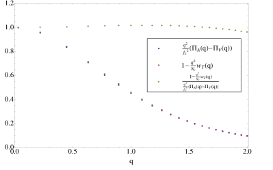
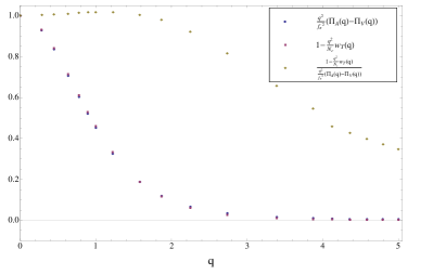
Figure 1: The numerical result of $1-{q^{2}\over N_{c}}w_{T}$, the difference of the vector and axial vector two-point functions $\left({q^{2}\over f_{\pi}^{2}}\left[\Pi_{A}(q)-\Pi_{V}(q)\right]\right)$ that appear in Eq.(4.35), and their ratio are plotted a a function of $q$, which is measured in units of $z_{\Lambda}^{-1}$ which is essentially $\Lambda_{QCD}$, defined in [12]. On the left, there is a zoom of the plot for small $q$ and on the right the whole plot is depicted until large values of $q$.

In Fig.(2), we plot the transverse part of the correlator, $1-{q^{2}\over N_{c}}w_{T}(q)$ for different values of the bare quark mass. The slopes of the curves in Fig.(2) for low momenta lead to the value of $C_{22}^{W}$ for different quark masses

$$\begin{split}&C_{22}^{W}=6.71\;10^{-3}GeV^{-2}\;\;\;\mbox{for}\;\;\;{m_{q}\over\Lambda_{QCD}}=0\\ &C_{22}^{W}=6.21\;10^{-3}GeV^{-2}\;\;\;\mbox{for}\;\;\;{m_{q}\over\Lambda_{QCD}}=0.0092\\ &C_{22}^{W}=4.45\;10^{-3}GeV^{-2}\;\;\;\mbox{for}\;\;\;{m_{q}\over\Lambda_{QCD}}=0.31\end{split}$$ (4.37)

where $C_{22}^{W}$ was defined in (4.36) and captures the low momentum asymptotics of the correlator. We have used $\Lambda_{QCD}=549\;MeV$, as found by the fit to meson spectra in [13]. The mass ${m_{q}\over\Lambda_{QCD}}=0.0092$ corresponds to ${m_{u}+m_{d}\over 2}$ as fit in [13]. The mass ${m_{q}\over\Lambda_{QCD}}=0.31$ corresponds to the mass of the strange quark again from the same fit.

Figure 2: The transverse part of the vector-axial vector correlator is plotted in terms of q for different bare quark masses. We used the values for the quark mass which were found by matching to the meson spectrum in [12] and [13].

The transverse part of the vector-axial vector correlator times $q^{2}/N_{c}$, for large momentum, is plotted in Fig.(3). We have not been able to derive analytically the large $q$ asymptotics of this correlator. We have therefore calculated it numerically and fitted a power law at sufficiently large $q$. As seen in Fig.(3), the subleading UV behavior of ${q^{2}\over N_{c}}w_{T}(q)$ is $1/q^{6}$, instead of the $1/q^{4}$ expected from QCD. This is not unexpected, and suggests that in the UV of the model we are using there are lighter stringy states (before the antisymmetric tensor) that contribute to the correlator and dominate its UV asymptotics.

We observe that the subleading behavior of the correlator is subleading to the expected QCD result. In [2], [3] the nonperturbative effect to the correlator was found by using operator product expansion as it is mentioned in the introduction. It was shown that for large momentum, the subleading part of $w^{QCD}_{T}$ is expected to be $\sim 1/q^{6}$, hence ${q^{2}\over N_{c}}w^{QCD}_{T}\sim 1/q^{4}$. By finding the best fit to our numerical data we find that the subleading term of ${q^{2}\over N_{c}}w_{T}$ is $\sim 1/q^{5.9974}$. This disagreement with QCD for large $q$ is suggesting that for the simplistic glue theory we are using , the fermionic operator in question does not appear in the appropriate OPE of the currents.

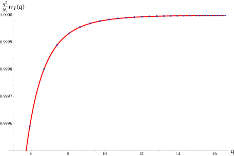
Figure 3: The numerical plot and the fit of the transverse part of the vector-axial vector correlator times $q^{2}/N_{c}$ in terms $q$, for large Euclidean momentum. The function that fits the numerical data is $1-{18.75\over q^{5.9974}}$. As usual $q$ is given in units of $\Lambda_{QCD}$ as defined in [12].

As it is shown in the next section the difference of the vector two point function from the axial one for large momentum is found to be similar to the QCD result which is $~{}1/q^{6}$, hence ${q^{2}\over N_{c}}(\Pi_{A}(q^{2})-\Pi_{V}(q^{2})\sim 1/q^{4}$. Therfore, Eq.(4.35) is violated for large momentum since our result for the vector-axial vector correlator gives $1-{q^{2}\over N_{c}}w_{T}\sim 1/q^{5.9974}$. A discussion of Eq.(4.35) in the context of QCD exists in [7]. The above outcome is similar to the result of the hard wall AdS/QCD model which is analyzed in Appendix B of [6].

5 Vector and Axial current-current correlators

We present here the vector and axial current-current correlators for large Euclidean momentum, following [24], [25]. Those have already been calculated analytically in the abelian case of our model in [13] and found to contain a subleading power of $1/q^{4}$, (for more details see Eqs.(4.18) and (F.11) of [13]) that is absent from QCD which predicts a $1/q^{6}$ subleading behavior. However it turns that the analytical approximations made were unreliable. Here we will calculate the difference numerically and show agreement with QCD.

The two-point functions are defined as

$$\int d^{4}xd^{4}ye^{iqx+ipy}\langle T\{J^{a}_{(V/A)\,\mu}(x)J^{b}_{(V/A)\,\nu}(y)\}\rangle=\delta^{ab}(q^{2}\eta_{\mu\nu}-q_{\mu}q_{\nu})\Pi_{V/A}(q^{2})(2\pi)^{4}\delta^{(4)}(p+q)$$ (5.38)

We now calculate $\Pi_{A}(q^{2})-\Pi_{V}(q^{2})$ numerically using the full equations of motion without any approximation. The result for low momentum is shown in Fig.1. The above difference is plotted in terms of $q$, Fig.(4), for large Euclidean momentum and we find that the function that fits the data is ${0.653\over q^{6.00933}}$. The difference of the axial vector and vector two point functions was calculated in QCD, using operator product expansion method, [31]. In the chiral limit the QCD result reads

$$\Pi_{A}(q^{2})-\Pi_{V}(q^{2})\sim{2\pi\alpha_{s}\over q^{6}}\langle(\bar{\psi}_{L}\gamma_{\mu}t^{a}\psi_{L})(\bar{\psi}_{R}\gamma_{\mu}t^{a}\psi_{R}))\rangle$$ (5.39)

whose leading power agrees with the numerical result of our calculation at large momenta.

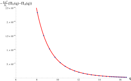
Figure 4: The numerical plot and the fit of the difference of the vector and axial vector 2 point functions. The fit reads ${0.653\over q^{6.00933}}$. As usual $q$ is given in units of $\Lambda_{QCD}$ as defined in [12].

6 Conclusions

In the present work, we have shown that the relation (4.35) which was proposed by Son and Yamamoto relating the vector-axial vector flavor current correlator in weak electric field to the difference of the vector and axial vector two point functions is valid only for low Euclidean momenta in the context of an AdS/QCD model with non-trivial dynamics for the chiral condensate.

For large momenta, this relation is no longer valid in our model. Moreover, the dependence of the $w_{T}$ correlator on $q^{2}$ for large $q^{2}$ is subleading to that expected from QCD.

We also notice that the difference of the vector and axial vector flavor current two-point functions in our model falls off as $q^{-6}$ for large $q^{2}$ as it is expected from the operator product expansion in QCD.

This computation could be sharpened by using a more realistic theory for the glue sector, like the Improved holographic QCD model, [9]. This investigation in underway.

7 Acknowledgements

We would like to thank A. Paredes for discussions.

This work was partially supported by European Union grants FP7-REGPOT-2008-1-CreteHEPCosmo-228644 and PERG07-GA-2010-268246. I. Iatrakis work was supported by the project ”HERAKLEITOS II - University of Crete” of the Operational Programme for Education and Lifelong Learning 2007 - 2013 (E.P.E.D.V.M.) of the NSRF (2007 - 2013), which is co-funded by the European Union (European Social Fund) and National Resources.

Note added

After this paper was in its last stages, [42] appeared that studied the same correlator in the soft wall model.

References

- [1] S. L. Adler and W. A. Bardeen, “Absence of higher order corrections in the anomalous axial vector divergence equation,” Phys. Rev. 182, 1517 (1969).
- [2] M. Knecht, S. Peris, M. Perrottet and E. De Rafael, “Electroweak hadronic contributions to the muon (g-2),” JHEP 0211 (2002) 003 [ArXiv:hep-ph/0205102].
- [3] A. Czarnecki, W. J. Marciano and A. Vainshtein, “Refinements in electroweak contributions to the muon anomalous magnetic moment,” Phys. Rev. D 67, 073006 (2003) [Erratum-ibid. D 73, 119901 (2006)] [ArXiv:hep-ph/0212229].
- [4] A. Vainshtein, “Perturbative and nonperturbative renormalization of anomalous quark triangles,” Phys. Lett. B 569, 187 (2003) [ArXiv:hep-ph/0212231].
- [5] M. Knecht, S. Peris, M. Perrottet and E. de Rafael, “New nonrenormalization theorems for anomalous three point functions,” JHEP 0403, 035 (2004) [ArXiv:hep-ph/0311100].
- [6] D. T. Son and N. Yamamoto, “Holography and Anomaly Matching for Resonances,” [ArXiv:1010.0718][hep-ph].
- [7] M. Knecht, S. Peris and E. de Rafael, “On Anomaly Matching and Holography,” [ArXiv:1101.0706][hep-ph].
- [8] T. Sakai, S. Sugimoto, “Low energy hadron physics in holographic QCD,” Prog. Theor. Phys. 113 (2005) 843-882. [ArXiv:hep-th/0412141].
-
[9]
U. Gursoy and E. Kiritsis,
“Exploring improved holographic theories for QCD: Part I,”
JHEP 0802 (2008) 032
[ArXiv:0707.1324][hep-th];
U. Gursoy, E. Kiritsis and F. Nitti, “Exploring improved holographic theories for QCD: Part II,” JHEP 0802 (2008) 019 [ArXiv:0707.1349][hep-th];
E. Kiritsis, “Dissecting the string theory dual of QCD,” Fortsch. Phys. 57 (2009) 396 [ArXiv:0901.1772][hep-th];
U. Gursoy, E. Kiritsis, L. Mazzanti, G. Michalogiorgakis and F. Nitti, “Improved Holographic QCD,” Lect. Notes Phys. 828 (2011) 79 [ArXiv:1006.5461][hep-th]. - [10] A. Sen, “Tachyon dynamics in open string theory,” Int. J. Mod. Phys. A 20 (2005) 5513 [ArXiv:hep-th/0410103].
- [11] R. Casero, E. Kiritsis and A. Paredes, “Chiral symmetry breaking as open string tachyon condensation,” [ArXiv:hep-th/0702155].
- [12] I. Iatrakis, E. Kiritsis and A. Paredes “An AdS/QCD model from Sen’s tachyon action,” [ArXiv:1003.2377][hep-ph].
- [13] I. Iatrakis, E. Kiritsis and A. Paredes “An AdS/QCD model from tachyon condensation: II,” JHEP 1011, 123 (2010) [ArXiv:1010.1364][hep-ph].
-
[14]
J. Erlich, E. Katz, D. T. Son and M. A. Stephanov,
“QCD and a holographic model of hadrons,”
Phys. Rev. Lett. 95 (2005) 261602
[ArXiv:hep-ph/0501128];
L. Da Rold and A. Pomarol, “Chiral symmetry breaking from five dimensional spaces,” Nucl. Phys. B 721 (2005) 79 [ArXiv:hep-ph/0501218]. - [15] A. Karch, E. Katz, D. T. Son and M. A. Stephanov, “Linear confinement and AdS/QCD,” Phys. Rev. D 74 (2006) 015005 [ArXiv:hep-ph/0602229].
-
[16]
L. Cappiello, O. Cata, G. D’Ambrosio,
“Antisymmetric tensors in holographic approaches to QCD,”
Phys. Rev. D82 (2010) 095008.
[ArXiv:1004.2497][hep-ph];
S. K. Domokos, J. A. Harvey and A. B. Royston, “Completing the framework of AdS/QCD: mesons and excited omega/rho’s,” JHEP 1105 (2011) 107 [ArXiv:1101.3315][hep-th];
R. Alvares, C. Hoyos and A. Karch, “An improved model of vector mesons in holographic QCD,” [ArXiv:1108.1191][hep-ph]. - [17] T. Imoto, T. Sakai, S. Sugimoto, “Mesons as Open Strings in a Holographic Dual of QCD,” Prog. Theor. Phys. 124 (2010) 263-284. [ArXiv:1005.0655][hep-th].
-
[18]
S. Kuperstein and J. Sonnenschein,
“Non-critical supergravity (d 1) and holography,”
JHEP 0407 (2004) 049
[ArXiv:hep-th/0403254];
- [19] S. Kuperstein and J. Sonnenschein, “Non-critical, near extremal AdS6 background as a holographic laboratory of four dimensional YM theory,” JHEP 0411 (2004) 026 [ArXiv:hep-th/0411009].
- [20] E. Witten, “Anti-de Sitter space and holography,” Adv. Theor. Math. Phys. 2 (1998) 253 [ArXiv:hep-th/9802150].
- [21] D. Z. Freedman, S. D. Mathur, A. Matusis and L. Rastelli, “Correlation functions in the CFT(d) / AdS(d+1) correspondence,” Nucl. Phys. B 546 (1999) 96 [ArXiv:hep-th/9804058].
- [22] A. Sen, “Dirac-Born-Infeld action on the tachyon kink and vortex,” Phys. Rev. D 68, 066008 (2003) [ArXiv:hep-th/0303057].
- [23] A. A. Tseytlin, “On nonAbelian generalization of Born-Infeld action in string theory,” Nucl. Phys. B 501 (1997) 41 [ArXiv:hep-th/9701125].
- [24] J. Erlich, E. Katz, D. T. Son and M. A. Stephanov, “QCD and a Holographic Model of Hadrons,” Phys. Rev. Lett. 95, 261602 (2005) [ArXiv:hep-ph/0501128].
- [25] L. Da Rold and A. Pomarol, “Chiral symmetry breaking from five dimensional spaces,” Nucl. Phys. B 721, 79 (2005) [ArXiv:hep-ph/0501218].
- [26] M. Kruczenski, D. Mateos, R. C. Myers and D. J. Winters, “Towards a holographic dual of large-N(c) QCD,” JHEP 0405, 041 (2004) [ArXiv:hep-th/0311270].
- [27] T. Takayanagi, S. Terashima and T. Uesugi, “Brane-antibrane action from boundary string field theory,” JHEP 0103, 019 (2001) [ArXiv:hep-th/0012210].
- [28] C. Kennedy and A. Wilkins, “Ramond-Ramond couplings on brane-antibrane systems,” Phys. Lett. B 464, 206 (1999) [ArXiv:hep-th/9905195].
- [29] P. Kraus and F. Larsen, “Boundary string field theory of the DD-bar system,” Phys. Rev. D 63, 106004 (2001) [ArXiv:hep-th/0012198].
- [30] J. Bijnens, L. Girlanda and P. Talavera, “The Anomalous chiral Lagrangian of order p**6,” Eur. Phys. J. C 23 (2002) 539 [ArXiv:hep-ph/0110400].
- [31] M. A. Shifman, A. I. Vainshtein and V. I. Zakharov, “QCD and Resonance Physics: Applications,” Nucl. Phys. B 147 (1979) 448.
- [32] J. Sonnenschein, “What does the string / gauge correspondence teach us about Wilson loops?,” [ArXiv:hep-th/0003032].
- [33] I. R. Klebanov and J. M. Maldacena, “Superconformal gauge theories and non-critical superstrings,” Int. J. Mod. Phys. A 19 (2004) 5003 [ArXiv:hep-th/0409133].
- [34] F. Bigazzi, R. Casero, A. L. Cotrone, E. Kiritsis and A. Paredes, “Non-critical holography and four-dimensional CFT’s with fundamentals,” JHEP 0510, 012 (2005) [ArXiv:hep-th/0505140].
- [35] T. Gherghetta, J. I. Kapusta and T. M. Kelley, “Chiral symmetry breaking in the soft-wall AdS/QCD model,” Phys. Rev. D 79, 076003 (2009) [ArXiv:0902.1998][hep-ph]; Y. Q. Sui, Y. L. Wu, Z. F. Xie and Y. B. Yang, “Prediction for the Mass Spectra of Resonance Mesons in the Soft-Wall AdS/QCD with a Modified 5D Metric,” Phys. Rev. D 81, 014024 (2010) [ArXiv:0909.3887][hep-ph].
- [36] J. P. Shock and F. Wu, “Three flavour QCD from the holographic principle,” JHEP 0608, 023 (2006) [ArXiv:hep-ph/0603142].
- [37] A. L. Cotrone, A. Dymarsky and S. Kuperstein, “On vector meson masses in a holographic SQCD” [ArXiv:1010.1017][hep-ph].
-
[38]
U. Gursoy, E. Kiritsis, L. Mazzanti and F. Nitti,
“Deconfinement and Gluon Plasma Dynamics in Improved Holographic QCD,”
Phys. Rev. Lett. 101, 181601 (2008)
[ArXiv:0804.0899][hep-th];
U. Gursoy, E. Kiritsis, L. Mazzanti and F. Nitti, “Holography and Thermodynamics of 5D Dilaton-gravity,” JHEP 0905 (2009) 033 [ArXiv:0812.0792 ][hep-th].
- [39] D. Kutasov, M. Marino and G. W. Moore, “Some exact results on tachyon condensation in string field theory,” JHEP 0010 (2000) 045. [ArXiv:hep-th/0009148]
- [40] T. Takayanagi, S. Terashima and T. Uesugi, “Brane-antibrane action from boundary string field theory,” JHEP 0103, 019 (2001) [ArXiv:hep-th/0012210].
- [41] M. Alishahiha, H. Ita and Y. Oz, “On superconnections and the tachyon effective action,” Phys. Lett. B 503 (2001) 181 [ArXiv:hep-th/0012222].
- [42] P. Colangelo, F. De Fazio, F. Giannuzzi, S. Nicotri and J. J. Sanz-Cillero, “Anomalous vertex function in the soft-wall holographic model of QCD,” [ArXiv:1108.5945][hep-ph].