Detection of negative effective magnetic pressure instability in turbulence simulations

Abstract

We present the first demonstration of the negative effective magnetic pressure instability in direct numerical simulations of stably stratified, externally forced, isothermal hydromagnetic turbulence in the regime of large plasma beta. By the action of this instability, an initially uniform horizontal magnetic field forms flux concentrations whose scale is large compared to the turbulent scale. We further show that the magnetic energy of these large-scale structures is only weakly dependent on the magnetic Reynolds number, provided its value is large enough for the instability to be excited. Our results support earlier mean-field calculations and analytic work which identified this instability. Applications to the formation of active regions in the Sun are discussed.

1. Introduction

The solar convection zone is highly turbulent and mixing is expected to be efficient. Nevertheless, the Sun displays coherent structures encompassing many turbulent eddy scales. A well-known example is the large-scale magnetic field of the Sun that is antisymmetric about the equator and shows a 22 year solar cycle (Stenflo & Vogel, 1986). Another prominent example in the Sun is the emergence of active regions. It is generally believed that active regions are the result of some non-axisymmetric instability of $\sim 100\,{\rm kG}$ magnetic fields in the tachocline (Gilman & Dikpati, 2000; Cally et al., 2003; Parfrey & Menou, 2007). However, the existence of such strong fields remains debatable (Brandenburg, 2005).

A powerful tool for understanding the emergence of such large-scale structures from a turbulent background is mean-field dynamo theory (Moffatt, 1978; Parker, 1979; Krause & Rädler, 1980). With the advent of powerful computers and numerical simulation tools, it has become possible to confront many of the mean-field predictions with direct simulations (Brandenburg & Subramanian, 2005). Here we consider the idea that statistically steady, stratified, hydromagnetic turbulence with an initially uniform magnetic field is unstable to the negative effective magnetic pressure instability (NEMPI). This instability is caused by the suppression of turbulent hydromagnetic pressure (the isotropic part of combined Reynolds and Maxwell stresses) by the mean magnetic field (Kleeorin et al., 1990; Rogachevskii & Kleeorin, 2007). At large Reynolds numbers and for sub-equipartition magnetic fields, the negative turbulent contribution can become so large that the effective mean magnetic pressure (the sum of turbulent and non-turbulent contributions) appears negative. In a stratified medium, this results in the excitation of NEMPI that causes formation of large-scale inhomogeneous magnetic structures. NEMPI is similar to the large-scale dynamo instability, except that it only redistributes the total magnetic flux, creating large-scale concentrated magnetic flux regions at the expense of turbulent kinetic energy.

Historically, the magnetic suppression of the Reynolds stress was first found by Rädler (1974) and Rüdiger (1974). Later, Rüdiger et al. (1986) considered the Maxwell stress and found the mean effective magnetic tension to be suppressed by mean fields. However, these calculations were based on quasi-linear theory which is only valid at low fluid and magnetic Reynolds numbers. Kleeorin et al. (1990, 1996) considered the combined Reynolds and Maxwell stresses at large Reynolds numbers and found a sign reversal of the effective mean magnetic pressure. This result is based on the $\tau$ approximation, and has been corroborated using the renormalization procedure (Kleeorin & Rogachevskii, 1994).

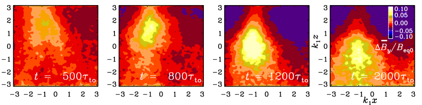
Figure 1.— $\Delta\overline{B}_{y}/B_{\rm eq0}$ in the $xz$ plane for $\mbox{\rm Re}_{M}=6$ and $B_{0}/B_{\rm eq0}=0.05$, showing a descending “potato sack” structure. Time is in units of $\tau_{\rm to}$ (lower right).

The magnetic suppression of the combined Reynolds and Maxwell stresses is quantified in terms of new turbulent mean-field coefficients that relate the components of the sum of Reynolds and Maxwell stresses to the mean magnetic field. These coefficients depend on the magnetic field and have now been determined in direct numerical simulations (DNS) for a broad range of different cases, including unstratified forced turbulence (Brandenburg et al., 2010), isothermally stratified forced turbulence (Brandenburg et al., 2011, hereafter BKKR), and turbulent convection (Käpylä et al., 2011). These simulations have clearly demonstrated that the mean effective magnetic pressure is negative for magnetic field strengths below about half the equipartition field strength. However, these DNS studies did not find the actual instability.

With a quantitative parameterization in place, it became possible to build mean-field models of stratified turbulence which clearly demonstrate exponential growth and saturation of NEMPI. In view of applications to the formation of active regions in the Sun, such simulations were originally done for an adiabatically stratified layer (Brandenburg et al., 2010). In addition, mean-field studies showed the existence of NEMPI even for isothermal stably stratified layers (Kemel et al., 2011). This last result turned out to be important because it paved the way for this Letter where we demonstrate NEMPI through DNS. Once we establish the physical reality of this effect, it would be important to apply it to realistic solar models which include proper boundary conditions, realistic stratification, convective flux, and radiation transport. However, at this stage it is essential to isolate NEMPI as a physical effect under conditions that are as simple as possible.

2. The model

We consider a domain of size $L_{x}\times L_{y}\times L_{z}$ in Cartesian coordinates, $(x,y,z)$, with periodic boundary conditions in the $x$ and $y$ directions and stress-free perfectly conducting boundaries at top and bottom ($z=\pm L_{z}/2$). The volume-averaged density is therefore constant in time and equal to its initial value, $\rho_{0}=\langle\rho\rangle$. We solve the equations for the velocity $U$, the magnetic vector potential $A$, and the density $\rho$,

$$\rho{{\rm D}{}\mbox{\boldmath$U$}{}\over{\rm D}{}t}=\mbox{\boldmath$J$}{}\times\mbox{\boldmath$B$}{}-c_{\rm s}^{2}\mbox{\boldmath$\nabla$}{}\rho+\mbox{\boldmath$\nabla$}{}\cdot(2\nu\rho\mbox{\boldmath${\sf S}$}{})+\rho(\mbox{\boldmath$f$}{}+\mbox{\boldmath$g$}{}),$$ (1)

$${\partial\mbox{\boldmath$A$}{}\over\partial t}=\mbox{\boldmath$U$}{}\times\mbox{\boldmath$B$}{}+\eta\nabla^{2}\mbox{\boldmath$A$}{},$$ (2)

$${\partial\rho\over\partial t}=-\mbox{\boldmath$\nabla$}{}\cdot\rho\mbox{\boldmath$U$}{},$$ (3)

where $\nu$ is kinematic viscosity, $\eta$ is magnetic diffusivity, $\mbox{\boldmath$B$}{}=\mbox{\boldmath$B$}{}_{0}+\mbox{\boldmath$\nabla$}{}\times\mbox{\boldmath$A$}{}$ is the magnetic field, $\mbox{\boldmath$B$}{}_{0}=(0,B_{0},0)$ is the imposed uniform field, $\mbox{\boldmath$J$}{}=\mbox{\boldmath$\nabla$}{}\times\mbox{\boldmath$B$}{}/\mu_{0}$ is the current density, $\mu_{0}$ is the vacuum permeability, ${\sf S}_{ij}={\textstyle{1\over 2}}(U_{i,j}+U_{j,i})-{\textstyle{1\over 3}}\delta_{ij}\mbox{\boldmath$\nabla$}{}\cdot\mbox{\boldmath$U$}{}$ is the traceless rate of strain tensor, and commas denote partial differentiation. The forcing function $f$ consists of random, white-in-time, plane non-polarized waves with an average wavenumber $k_{\it f}=15\,k_{1}$, where $k_{1}=2\pi/L_{z}$ is the lowest wavenumber in the domain. The forcing strength is such that the turbulent rms velocity is approximately independent of $z$ with $u_{\rm rms}=\langle\mbox{\boldmath$u$}{}^{2}\rangle^{1/2}\approx 0.1\,c_{\rm s}$. The gravitational acceleration $\mbox{\boldmath$g$}{}=(0,0,-g)$ is chosen such that $k_{1}H_{\rho}=1$, which leads to a density contrast between bottom and top of $\exp(2\pi)\approx 535$. Here, $H_{\rho}=c_{\rm s}^{2}/g$ is the density scale height.

Our simulations are characterized by the fluid Reynolds number $\mbox{\rm Re}\equiv u_{\rm rms}/\nu k_{\it f}$, the magnetic Prandtl number $\mbox{\rm Pr}_{M}=\nu/\eta$ and the magnetic Reynolds number $\mbox{\rm Re}_{M}\equiv\mbox{\rm Re}\,\mbox{\rm Pr}_{M}$. Following earlier work (Brandenburg et al., 2011), we choose $\mbox{\rm Pr}_{M}=0.5$ and $\mbox{\rm Re}_{M}$ in the range $0.7$–$74$. The magnetic field is expressed in units of the local equipartition field strength near the top, $B_{\rm eq}=\sqrt{\mu_{0}\rho}\,u_{\rm rms}$, while $B_{0}$ is specified in units of the averaged value, $B_{\rm eq0}=\sqrt{\mu_{0}\rho_{0}}\,u_{\rm rms}$. We monitor $\Delta\overline{B}_{y}=\overline{B}_{y}-B_{0}$, where $\overline{B}_{y}$ is an average over $y$ and a certain time interval $\Delta t$. Time is expressed in eddy turnover times, $\tau_{\rm to}=(u_{\rm rms}k_{\it f})^{-1}$. Occasionally, we also consider the turbulent-diffusive timescale, $\tau_{\rm td}=(\eta_{\rm t0}k_{1}^{2})^{-1}$, where $\eta_{\rm t0}=u_{\rm rms}/3k_{\it f}$ is the estimated turbulent magnetic diffusivity. Another diagnostic quantity is the rms magnetic field in the $k=k_{1}$ Fourier mode, $B_{1}$, which is here taken as an average over $2\leq k_{1}z\leq 3$, and is close to the top at $k_{1}z=\pi$. (Note that $B_{1}$ does not include the imposed field $B_{0}$ at $k=0$.)

Figure 2.— Dependence of $B_{1}/B_{\rm eq}$ (averaged over $2\leq k_{1}z\leq 3$) on $\mbox{\rm Re}_{M}$ for $B_{0}/B_{\rm eq0}=0.05$.

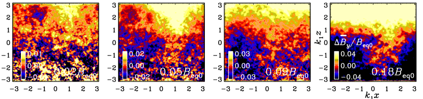
Figure 3.— $\Delta\overline{B}_{y}/B_{\rm eq0}$ in the $xz$ plane for $\mbox{\rm Re}_{M}=36$ and $B_{0}/B_{\rm eq0}=0.02$, 0.05, 0.09, and 0.18.

The simulations are performed with the Pencil Code, which uses sixth-order explicit finite differences in space and a third-order accurate time stepping method. We use numerical resolutions of $128^{3}$ and $256^{3}$ mesh points when $L_{x}=L_{y}=L_{z}$, and $1024\times 128^{2}$ when $L_{x}=8L_{y}=8L_{z}$. To capture mean-field effects on the slower turbulent-diffusive timescale, which is $\tau_{\rm td}/\tau_{\rm to}=3k_{\it f}^{2}/k_{1}^{2}$ times slower than the dynamical timescale, we perform simulations for several thousand turnover times.

3. Results

The NEMPI phenomenon is already quite pronounced at intermediate values of $\mbox{\rm Re}_{M}\mathrel{\mathchoice{\vbox{\offinterlineskip\halign{\hfil$\displaystyle#$\hfil\cr>\cr\sim\cr}}}{\vbox{\offinterlineskip\halign{\hfil$\textstyle#$\hfil\cr>\cr\sim\cr}}}{\vbox{\offinterlineskip\halign{\hfil$\scriptstyle#$\hfil\cr>\cr\sim\cr}}}{\vbox{\offinterlineskip\halign{\hfil$\scriptscriptstyle#$\hfil\cr>\cr\sim\cr}}}}3$; see Figure 1, where we show $B_{y}$ averaged over $y$ and $\Delta t\approx 80\tau_{\rm to}$ (denoted by $\overline{B}_{y}$) at selected times during the first 2000 turnover times. The $\mbox{\rm Re}_{M}$ dependence of $B_{1}/B_{\rm eq}$ is shown in Figure 2. For $\mbox{\rm Re}_{M}>3$, the $\mbox{\rm Re}_{M}$ dependence is relatively weak, which suggests that NEMPI is a genuine high Reynolds number effect.

The results for the case of $\mbox{\rm Re}_{M}=6$ show strong similarities to earlier mean-field simulations. During the first 500 turnover times, flux concentrations form first near the surface, but at later times the location of the peak magnetic field moves gradually downward. This phenomenon is a direct consequence of the negative effective magnetic pressure, making such structures heavier than their surroundings. Their shape resembles that of a falling “potato sack” and has been seen in numerous mean-field calculations during the nonlinear stage of NEMPI (Brandenburg et al., 2010; Käpylä et al., 2011). Using the technique described in BKKR, we have found that for $\mbox{\rm Re}_{M}\mathrel{\mathchoice{\vbox{\offinterlineskip\halign{\hfil$\displaystyle#$\hfil\cr>\cr\sim\cr}}}{\vbox{\offinterlineskip\halign{\hfil$\textstyle#$\hfil\cr>\cr\sim\cr}}}{\vbox{\offinterlineskip\halign{\hfil$\scriptstyle#$\hfil\cr>\cr\sim\cr}}}{\vbox{\offinterlineskip\halign{\hfil$\scriptscriptstyle#$\hfil\cr>\cr\sim\cr}}}}1.1$ and $\mbox{\rm Pr}_{M}=0.5$, the effective magnetic pressure has a negative minimum.

As expected from theory and mean-field calculations, NEMPI is only excited in a certain range of field strengths. In particular, only for $B_{0}/B_{\rm eq0}$ between 0.02 and 0.2 do we see large-scale magnetic structures. This is shown in Figure 3, where we see $B_{y}$, again averaged over $y$ and a time interval $\Delta t\approx 800\tau_{\rm to}$, in which the field is statistically steady. The clearest flux structure formations are seen for $B_{0}/B_{\rm eq0}\approx 0.05$. However, even for this case the flux concentrations are barely visible in a single snapshot. This has been one of the reasons why NEMPI has not been noticed before in DNS. An additional handicap was that the simulations of BKKR used a smaller scale separation ratio of only 5, which is nevertheless still sufficient for determining the governing mean-field coefficients and allows one to reach larger values of $\mbox{\rm Re}_{M}$.

Figure 4.— Bifurcation diagram showing $B_{1}/B_{\rm eq}$ vs. $B_{0}/B_{\rm eq0}$ (and vs. $B_{0}/B_{\rm eq}$ on the upper abscissa) for $\mbox{\rm Re}_{M}=36$.

Figure 5.— Slow exponential growth of the mean magnetic field in $2\leq k_{1}z\leq 3$ for $B_{0}/B_{\rm eq0}=0.05$, corresponding to $B_{0}/B_{\rm eq}=0.16$, for $\mbox{\rm Re}_{M}=36$ (solid line). The growth rate is $\approx 0.4\eta_{\rm t0}k_{1}^{2}$ (dotted line). Note that the total rms field, $B_{\rm rms}/B_{\rm eq}$ (dotted line) saturates much faster, as indicated by to upper abscissa.

In Figure 4 we plot $B_{1}/B_{\rm eq}$ as a function of $B_{0}/B_{\rm eq0}$, showing a peak at $B_{0}/B_{\rm eq0}\approx 0.05$. We recall that $B_{\rm eq}$ applies here to the location $2\leq k_{1}z\leq 3$ where $B_{1}$ has been evaluated, and there we have $B_{\rm eq}/B_{\rm eq0}\approx 0.3$. The fact that large-scale flux concentrations develop only for a certain range of imposed field strengths supports our interpretation that they are caused by NEMPI and not, for example, by some yet unknown dynamo mechanism. In all these cases, $\mbox{\boldmath$B$}{}-\mbox{\boldmath$B$}{}_{0}$ grows rapidly and reaches a saturation field strength that is independent of $\mbox{\boldmath$B$}{}_{0}$, provided $\mbox{\rm Re}_{M}\geq 35$. This suggests that this field is produced by small-scale dynamo action and not just by field line tangling. Another piece of evidence of the physical reality of NEMPI is shown in Figure 5, where we see that $B_{1}$ does indeed increase exponentially for the first 2000 turnover times, corresponding to about $3\tau_{\rm td}$. The growth rate is $\approx 0.4\eta_{\rm t0}k_{1}^{2}$, which is much less than $\tau_{\rm to}^{-1}$, but entirely compatible with mean-field calculations (BKKR; Käpylä et al., 2011).

Finally, to investigate the effects of the domain aspect ratio on the instability, we perform a calculation with $B_{0}/B_{\rm eq0}=0.05$, $\mbox{\rm Re}_{M}=36$, and change $L_{x}$ to $16\pi/k_{1}$. We find that the most unstable mode has a wavelength approximately equal to $L_{z}\approx 6H_{\rho}$. This result is also in agreement with mean-field models (e.g., Fig. 14 of Käpylä et al., 2011). The large-scale flux concentrations have an amplitude of only $\approx 0.1B_{\rm eq}$ and are therefore not seen in single snapshots, where the field reaches peak strengths comparable to $B_{\rm eq}$. Furthermore, as for any linear instability, the flux concentrations form a repetitive pattern, but this might be an artifact of idealized conditions.

4. Conclusions and discussion

The present simulations have, for the first time, demonstrated conclusively that NEMPI can operate in hydromagnetic turbulence under proper conditions, namely, strong stratification, sufficient scale separation (here $k_{\it f}/k_{1}=15$), and a mean field in an optimal range (here $\approx 0.15B_{\rm eq}$; see Figure 4). This instability has so far only been seen in mean-field simulations. By contrast, the present simulations are completely free of any mean-field consideration.

The instability is argued to be a consequence of the reduction of turbulent hydromagnetic pressure by a mean magnetic field and can be understood as follows (Kleeorin et al., 1996). The combined Reynolds and Maxwell stress is $\overline{\rho u_{i}u_{j}}-\overline{b_{i}b_{j}}/\mu_{0}+\delta_{ij}\overline{\mbox{\boldmath$b$}{}^{2}}/2\mu_{0}$, where $u$ and $b$ are velocity and magnetic fluctuations, respectively, and overbars indicate averaging. For isotropic turbulence, the turbulent hydromagnetic pressure is then $P_{\rm turb}={\textstyle{1\over 3}}(\overline{\rho\mbox{\boldmath$u$}{}^{2}}+\overline{\mbox{\boldmath$b$}{}^{2}}/2\mu_{0})$. On the other hand, the total turbulent energy $E_{\rm turb}\equiv{\textstyle{1\over 2}}(\overline{\rho\mbox{\boldmath$u$}{}^{2}}+\overline{\mbox{\boldmath$b$}{}^{2}}/\mu_{0})$, is nearly conserved because a uniform mean magnetic field does not perform any work; see Brandenburg et al. (2010) for a numerical demonstration. The presence of an additional 1/2 factor in front of the $\overline{\mbox{\boldmath$b$}{}^{2}}/\mu_{0}$ term in the expression for $P_{\rm turb}$, but not in that for $E_{\rm turb}$, implies that the generation of magnetic fluctuations results in a reduction of $P_{\rm turb}$, i.e. $P_{\rm turb}={\textstyle{1\over 3}}(2E_{\rm turb}-\overline{\mbox{\boldmath$b$}{}^{2}}/2\mu_{0})$. For anisotropic turbulence this negative contribution becomes larger. This physical effect is independent of stratification, but to obtain an instability one needs strong stratification.

We speculate that, in the solar context, NEMPI plays a role in formation of active regions from mean fields generated by the solar dynamo. Let us now ask whether this instability alone can describe the formation of active regions at the solar surface. Clearly, the flux concentrations we observe are not strong enough to be noticeable without averaging, while the active regions in the Sun are seen without averaging. This suggests that there may be additional mechanisms at work. One possibility is that of the magnetic suppression of the convective heat flux that has been invoked to explain the formation of sunspots (Kitchatinov & Mazur, 2000).

When the mean magnetic field becomes larger than the equipartition field strength, i.e., when NEMPI does not work, and the characteristic spatial scale of the magnetic field is smaller than the density height, it is instead the Parker magnetic buoyancy instability (Parker, 1966) that is excited.

The presence of a vertical field might also have a strong effect. Indeed simulations of convection with an imposed vertical field have produced a segregation into magnetized and unmagnetized regions (Tao et al., 1998; Kitiashvili et al., 2010) with formation of flux concentrations strong enough to be noticeable even without averaging. On the other hand NEMPI might become more powerful at stronger stratification. Increased stratification clearly has an enhancing effect on the growth rate (Kemel et al., 2011), but the effect on the saturation level has not yet been quantified. Furthermore, the interplay between NEMPI and the other effects also needs to be investigated.

Our work has established a close link between what can be expected from mean-field studies and what actually happens in DNS. This correspondence is particularly important because DNS cannot reach solar parameters in any conceivable future. Hence a deeper understanding of solar convection can only emerge by studying mean-field models on the one hand and to determine turbulent mean-field coefficients from simulations on the other hand. This concerns not only the dependence of the mean-field coefficients on parameters such as magnetic Reynolds and Prandtl numbers and scale separation ratio, but also the details of the source of turbulence. In particular, it has already been shown that the negative effective magnetic pressure effect is not unique to forced turbulence, but it also occurs in turbulent convection Käpylä et al. (2011), and thus in an unstably stratified layer. We emphasize that the present work demonstrates the predictive power of mean-field theory at an advanced level where quasi-linear theory fails (Rüdiger et al., 2011) but the spectral $\tau$ approach (Rogachevskii & Kleeorin, 2007) has proven useful.

More work using mean-field models is needed to elucidate details of the mechanism of NEMPI. For example, naive thinking suggests that the onset of NEMPI should occur at the depth where the effective magnetic pressure is minimum, but both mean-field models and DNS show that this is not the case. At least at early times, NEMPI appears most pronounced at the top of the domain, while the effective magnetic pressure is usually most negative at the bottom. On the other hand, the instability is a global one and local considerations such as these are not always meaningful. Another question is what happens when the imposed field is replaced by a dynamo-generated one. In that case, the turbulence may be helical and new terms involving current density can occur in the expression for the mean-field stress. Again, such possibilities are best studied using first the mean-field approach.

References

- Brandenburg (2005) Brandenburg, A. 2005, ApJ, 625, 539
- Brandenburg et al. (2011) Brandenburg, A., Kemel, K., Kleeorin, N., & Rogachevskii, I. 2011, ApJ, submitted (arXiv:1005.5700) (BKKR)
- Brandenburg et al. (2010) Brandenburg, A., Kleeorin, N., & Rogachevskii, I. 2010, Astron. Nachr., 331, 5
- Brandenburg & Subramanian (2005) Brandenburg, A., & Subramanian, K. 2005, Phys. Rep., 417, 1
- Cally et al. (2003) Cally, P. S., Dikpati, M., & Gilman, P. A. 2003, ApJ, 582, 1190
- Gilman & Dikpati (2000) Gilman, P. A., & Dikpati, M. 2000, ApJ, 528, 552
- Käpylä et al. (2011) Käpylä, P. J., Brandenburg, A., Kleeorin, N., Mantere, M. J., & Rogachevskii, I. 2011, MNRAS, submitted (arXiv:1105.5785)
- Kemel et al. (2011) Kemel, K., Brandenburg, A., Kleeorin, N., & Rogachevskii, I. 2011, Astron. Nachr., submitted (arXiv:1107.2752)
- Kitchatinov & Mazur (2000) Kitchatinov, L.L., & Mazur, M.V. 2000, Solar Phys., 191, 325
- Kitiashvili et al. (2010) Kitiashvili, I. N., Kosovichev, A. G., Wray, A. A., & Mansour, N. N. 2010, ApJ, 719, 307
- Kleeorin et al. (1996) Kleeorin, N., Mond, M., & Rogachevskii, I. 1996, A&A, 307, 293
- Kleeorin & Rogachevskii (1994) Kleeorin, N., & Rogachevskii, I. 1994, Phys. Rev. E, 50, 2716
- Kleeorin et al. (1990) Kleeorin, N.I., Rogachevskii, I.V., & Ruzmaikin, A.A. 1990, Sov. Phys. JETP, 70, 878
- Krause & Rädler (1980) Krause, F., & Rädler, K.-H. 1980, Mean-field Magnetohydrodynamics and Dynamo Theory (Oxford: Pergamon Press)
- Moffatt (1978) Moffatt, H.K. 1978, Magnetic Field Generation in Electrically Conducting Fluids (Cambridge: Cambridge Univ. Press)
- Parfrey & Menou (2007) Parfrey, K. P., & Menou, K. 2007, ApJ, 667, L207
- Parker (1966) Parker, E.N. 1966, ApJ, 145, 811
- Parker (1979) Parker, E.N. 1979, Cosmical magnetic fields (Oxford University Press, New York)
- Rädler (1974) Rädler, K.-H. 1974, Astron. Nachr., 295, 265
- Rogachevskii & Kleeorin (2007) Rogachevskii, I., & Kleeorin, N. 2007, Phys. Rev. E, 76, 056307
- Rüdiger (1974) Rüdiger, G. 1974, Astron. Nachr., 295, 275
- Rüdiger et al. (2011) Rüdiger, G., Kitchatinov, L. L., & Schultz, M., 2011, A&A, submitted (arXiv:1109.3345)
- Rüdiger et al. (1986) Rüdiger, G., Tuominen, I., Krause, F., Virtanen, H. 1986, A&A, 166, 306
- Stenflo & Vogel (1986) Stenflo, J. O., & Vogel, M. 1986, Nature, 319, 285
- Tao et al. (1998) Tao, L., Weiss, N. O., Brownjohn, D. P., & Proctor, M. R. E. 1998, ApJ, 496, L39