Audio mixing in a tri-port nano-electro-mechanical device

Abstract

We report on experiments performed on a cantilever-based tri-port nano-electro-mechanical (NEMS) device. Two ports are used for actuation and detection through the magnetomotive scheme, while the third port is a capacitively coupled gate electrode. By applying a low frequency voltage signal on the gate, we demonstrate mixing in the mechanical response of the device, even for low magnetomotive drives, without resorting to conduction measurements through the NEMS. The technique can thus be used in particular in the linear regime, as an alternative to nonlinear mixing, for normal conducting devices. An analytic theory is presented reproducing the data without free parameters.

Signal mixing is a very important tool of signal processing in conventional electronics. The basic application consists in translating an audio signal (typ. 0.01 - 15 kHz) into the radio-frequency bandwidth (10 - 100 MHz), enabling thus a straightforward broadcasting and multiplexing. Nowadays, nano-electro-mechanical (NEMS) devices based on silicon technologies routinely reach frequencies ranging from 1 up to 100 MHz someone1 ; someone2 , and can thus be thought of as potential components for electronic circuits.

The first works on nanomechanical mixing used an intrinsic nonlinearity of the device mix . The NEMS under study had a normal metal conducting layer, and needed to be used in its nonlinear dynamic range, under large deflections. Another scheme combines a gate capacitance driven at high frequencies close to resonance, with a semiconducting property of the device itself driven at low frequency McEuen . This method proves to be extremely useful for detecting the motion itself of very high frequency nanotube-based devices, through the imprint of the mixing effect in the conductance vanderzant . It has been developed since, with the adjunction of the field effect purcell and the impressive achievement of the “nano-radio” radio .

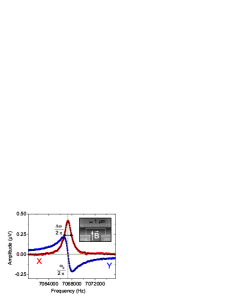
Figure 1: (Color online) The $X$ and $Y$ components (dots) for the bare resonance line measured in vacuum at 4.2 K with a magnetic field $B$ of 840 mT and a drive current amplitude $I_{0}=0.47$ $\mu$A (grounded gate voltage). The resulting displacement amplitude is $x_{0}=5.6$ nm. Lines are Lorentzian fits, leading to $\omega_{0}/2\pi=7.067$ MHz (position) and $\Delta\omega/2\pi=1.45$ kHz (linewidth). Inset: SEM image of the sample with indicated the direction of the static magnetic field.

In this paper we present a capacitive mixing scheme which applies to normal conducting NEMS kept in their linear regime. The device we use is the goal-post shaped silicon device presented in Ref. qfsus . It consists in two “feet” linked by a “paddle” of length $l\approx 7$ $\mu$m and thicknesses 150 nm, coupled to a large gate electrode. It has been fabricated from a thick SOI substrate, with the adjunction of a 30 nm aluminum layer on top. The drive and detection schemes use the magnetomotive technique: the paddle lies in a perpendicular, in plane, static field $B$ while an oscillating current $I_{0}\cos(\omega_{\rm rf}t)$ is fed through it. An alternating force of amplitude $F_{0}=I_{0}lB$, that we keep small, excites the first (out-of-plane) mode of the structure at an amplitude $x_{0}$, when $\omega_{\rm rf}\approx\omega_{0}$ ($\omega_{0}$ being the mode resonance frequency). The motion induces in turn a voltage $lB\omega_{\rm rf}x_{0}\cos(\omega_{\rm rf}t+\phi)$ that we detect with a lock-in amplifier referenced at $\omega_{\rm rf}$ ($X=lB\,\omega_{\rm rf}x_{0}\cos(\phi)$ and $Y=lB\,\omega_{\rm rf}x_{0}\sin(\phi)$ components). Experiments are performed at 4.2 K in cryogenic vacuum ($P<10^{-6}$mbar). In Fig. 1 we present a measured reference resonance line together with an SEM picture of the device. Note the quality of the Lorentzian fits proving excellent linearity.

On the gate electrode we apply a time-dependent voltage $V_{g}(t)=V_{g0}\cos(\omega_{\rm s}t)$, with $\omega_{\rm s}\ll\omega_{\rm rf}$. This drive generates an additional out-of-plane force $F_{g}(t)=(1/2)V_{g}(t)^{2}\partial C(x)/\partial x$ on the moving structure, $C$ being the total capacitance between the NEMS and the fixed electrode. This force is highly nonlinear, and at first order $\partial C(x)/\partial x\approx\partial C(x=0)/\partial x+[\partial^{2}C(x=0)/\partial x^{2}]\,x$. We have extremely carefully calibrated our device, demonstrating in particular that the first $\partial C(x=0)/\partial x$ term, which only creates a static shift in the structure’s rest position, can be safely neglected JAP . The equation of motion thus takes the form:

$$m\,\ddot{x}+2\Lambda\,\dot{x}+\left[k+\delta k\left(1+\cos[2\omega_{\rm s}t]\right)\right]\,x=F_{0}\cos(\omega_{\rm rf}t),$$ (1)

where $\delta k=-({1}/{4})V_{g0}^{2}\,{\partial^{2}C(x=0)}/{\partial x^{2}}$, $m$, $k$, and $\Lambda$ are the normal mass, the spring constant, and the damping constant of the mode under study, respectively. By definition $\omega_{0}=\sqrt{k/m}$ is the “bare” resonance frequency and $\Delta\omega=2\Lambda/m$ the full linewidth at half height on the lock-in $X$ component (both in Rad/s).

The problem at hand is a forced Mathieu equation. The homogeneous case ($F_{0}=0$) has been studied in details in the literature NafiafBook . To find the stationary solution of the inhomogeneous equation (1) we introduce an ansatz for $x(t)$:

$$x(t)=\sum_{n=-\infty}^{+\infty}|A_{n}|\cos(\omega_{\rm rf}t+2n\omega_{\rm s}t+{\rm arg}(A_{n}))\,,$$ (2)

with $A_{n}$ complex coefficients. Substitution of Eq. (2) into Eq. (1) gives the following recurrence equation:

$$a_{n}(\omega_{\rm rf})A_{n}+A_{n+1}+A_{n-1}=\delta_{n,0}\,2F_{0}/\delta k\,,$$ (3)

where we introduced: $a_{n}(\omega_{\rm rf})={\cal L}(\omega_{\rm rf}+2n\omega_{\rm s})2(k+\delta k)/\delta k$, with ${\cal L}(\omega)=(\omega_{\rm g}^{2}-\omega^{2}-i\omega\,\Delta\omega)/\omega_{\rm g}^{2}$, and $\omega_{\rm g}^{2}=(k+\delta k)/m$ the renormalized resonating frequency squared. Here $\delta_{i,j}$ is the Kronecker’s symbol. Our measurement scheme allows to measure the response of the device at the $\omega_{\rm rf}$ tone, but as it is clear from the form of $x(t)$, many other harmonics are present. What is obtained from the measurement of $X$ and $Y$ is the real and imaginary parts of $A_{0}$. An explicit expression of $A_{0}$ can be given in terms of continued fractions :

$$A_{0}=\frac{2F_{0}/\delta k}{a_{0}-\frac{1}{a_{1}-}\frac{1}{a_{2}-}\frac{1}{a_{3}-}\cdots-\frac{1}{a_{-1}-}\frac{1}{a_{-2}-}\frac{1}{a_{-3}-}\cdots}\,.$$ (4)

With no mixing ($\delta k\rightarrow 0$), Eq. (4) reduces to the standard harmonic Lorentzian solution $A_{0}=2F_{0}/a_{0}\delta k=F_{0}/[m\,\omega_{\rm g}^{2}{\cal L}(\omega_{\rm rf})]$. For non-vanishing $\delta k$ the effect of the mixing is to induce sidebands in the response function at intervals of frequency $2\omega_{\rm s}/2\pi$.

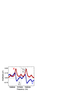
Figure 2: (Color online) Measurement of the $X$ an $Y$ components (red and blue dots) with a magnetomotive drive of $I_{0}=0.93$ $\mu$A and $B=840$ mT in presence of a gate modulation of frequency $\omega_{s}=2$ kHz and voltage $V_{g0}=$ 1.4 V (implying $\delta k/k=2.\times 10^{-3}$). The lines are our theoretical predictions.

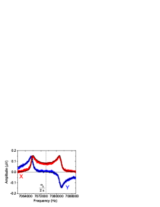
Figure 3: (Color online) Same as Fig. 2 with $\omega_{s}=5$ Hz.

In Fig. 2 we present the measured data for a gate modulation signal $V_{g0}$ of 1.4 V and a frequency of 2 kHz. The magnetomotive drive is kept in the linear regime. The lines are calculated numerically from Eq. (4) taking into account 50 nested fractions in the recursion (each fraction adds one pole at positive frequency to the response function). We found however that for these values of the parameters adding more than 5 terms in the recursive expression does not change visually the result. All numerical parameters ($m$, $\partial^{2}C(x=0)/\partial x^{2}$, etc…) are obtained from the careful calibration of the setup JAP : there are thus no free parameters in the theoretical prediction. The agreement is excellent, and one can clearly distinguish in the $X$ signal the peaks separated by $2\omega_{\rm s}/2\pi$.

The behavior presented in Fig. 2 is representative for values of $\omega_{\rm s}\gg\Delta\omega$. In the opposite limit we found that the peaks in the $X$ signal merge together to form a characteristic structure of hat shape. The experimental results are shown in Fig. 3, where the gate modulation frequency $\omega_{\rm s}/2\pi=5$ Hz. Also in this case the theory works perfectly well, but one needs to include 50 nested fractions to reach convergence. A simple solution can be actually found in this limit. The gate modulation is so slow that the oscillator reaches the stationary oscillation state before the gate changes of an appreciable quantity. In practice focusing on the $X$ signal one would see a lorentzian peak that bounces back and forth in the frequency plot around $\omega_{\rm rf}$ with an amplitude of $\delta k/2\pi m$. Since the measurement averages over a time longer than $1/\omega_{\rm s}$ (typ. 1 s) the result is this hat shaped plot shown in Fig. 3. An analytical expression for this can be readily found by averaging the quasi-stationary value of $A_{0}$ over a period $2\pi/\omega_{\rm s}$. This gives:

$$A_{0}={F_{0}\over m\omega_{\rm g}^{2}}\int_{0}^{2\pi/2\omega_{\rm s}}\!\!\!\!\!\!\!\!\!\!\!\!\!\!\!\!\!\frac{(2\omega_{\rm s}/2\pi)\,dt}{{\cal L}(\omega_{\rm rf})+\frac{\delta k}{k+\delta k}\cos(2\omega_{\rm s}t)}=\frac{F_{0}}{m\omega_{\rm g}^{2}}f\left(\frac{a_{0}}{2}\right)\,,$$ (5)

with $f(z)={\rm sign}({\rm Re}[z])/\sqrt{z^{2}-1}$. We found that this expression coincides with the exact expression, Eq. (4), with 50 nested fractions for the case of Fig. 3.

We finally illustrate the overall behavior on Figs. 4 and 5. In both graphs we plot the height of the first poles, defined as the amplitude of the signal measured at $\omega_{\rm g}\pm 2n\omega_{\rm s}$ ($n=0,1,2$). In Fig. 4 we present the pole height dependence as a function of the modulation frequency (fixed $V_{g0}=1.4$ V), while in Fig. 5 we present the modulation amplitude dependence (fixed $\omega_{\rm s}/2\pi$=1.5 kHz). The lines are our theoretical predictions, with no free parameters, proving excellent agreement.

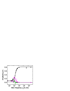
Figure 4: (Color online) Measured (dots) and predicted (lines) heights of the first poles as a function of the modulation frequency $\omega_{\rm s}/2\pi$ (same parameters as Fig. 2).

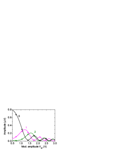
Figure 5: (Color online) Measured (dots) and predicted (lines) heights of the first poles as a function of the modulation amplitude $V_{g0}$ (same parameters as Fig.  2).

In conclusion, we presented a mixing technique that does not require a nonlinear drive of the nanomechanical device. The measure is performed with the standard magnetomotive technique, and does not require transport measurements to be performed. We present the analytic theory describing the results. Data are reproduced without free parameters, using the NEMS carefully measured characteristics. We demonstrate excellent understanding of the NEMS dynamics, and believe that our results will lead to future works in nanomechanical mixing.

- (1) J. S. Aldridge and A. N. Cleland, Phys. Rev. Lett. 94, 156403 (2005).
- (2) R. B. Karabalin, X. L. Feng, and M. L. Roukes, Nano Letters 9, 3116 (2009).
- (3) A. Erbe, H. Krömmer, A. Kraus, R. H. Blick, G. Corso and K. Richter Appl. Phys. Lett. 77, 3102 (2000); A. Erbe and R. Blick, IEEE Transactions on Ultrasonics, Ferroelectrics, and Frequency Control 49 1114 (2002).
- (4) Vera Sazonova, Yuval Yaish, Hande Ustünel, David Roundy, Tomás A. Arias & Paul L. McEuen, Nature 431, 284 (2004).
- (5) Benoit Witkamp, Menno Poot, and Herre S. J. van der Zant, Nano Letters 6, 2904 (2006).
- (6) S. T. Purcell, P. Vincent, C. Journet et V. T. Binh, Phys. Rev. Lett. 89, 276103 (2002).
- (7) K. Jensen, J. Weldon, H. Garcia and A. Zettl, Nano Letters 7, 3508 (2007).
- (8) E. Collin, T. Moutonet, J.-S. Heron, O. Bourgeois, Yu.M. Bunkov, H. Godfrin, J. of Low Temp. Phys. 162, 653 (2011).
- (9) E. Collin et. al, submitted to J. of Applied Phys. (2011).
- (10) A. H. Nayfeh and D. T. Mook, Nonlinear oscillations, Wiley (1995).