Dynamics of interacting qubits coupled to a common bath: Non-Markovian quantum state diffusion approach

Xinyu Zhao111Email:xzhao1@stevens.edu, Jun Jing, Brittany Corn and Ting Yu222Email:Ting.Yu@stevens.edu Center for Controlled Quantum Systems and the Department of Physics and Engineering Physics, Stevens Institute of Technology, Hoboken, New Jersey 07030, USA
Abstract

Non-Markovian dynamics is studied for two interacting quibts strongly coupled to a dissipative bosonic environment. For the first time, we have derived the non-Markovian quantum state diffusion (QSD) equation for the coupled two-qubit system without any approximations, and in particular, without the Markov approximation. As an application and illustration of our derived time-local QSD equation, we investigate the temporal behavior of quantum coherence dynamics. In particular, we find a strongly non-Markovian regime where entanglement generation is significantly modulated by the environmental memory. Additionally, we studied the residual entanglement in the steady state by analyzing the steady state solution of the QSD equation. Finally, we have discussed an approximate QSD equation.

pacs:
03.65.Yz, 03.67.Bg, 03.65.Ud, 32.90.+a

I Introduction

The theory of quantum open systems has attracted growing attention because the framework of system plus environment has become a fundamental paradigm in quantum dissipative system, quantum optics and quantum information science Openbook1 ; Openbook2 . In reality, no quantum systems can be completely isolated from their environment. The mutual interaction between the system and environment is responsible for many important physical processes such as dissipation, fluctuation, as well as decoherence and disentanglement. Quantum open system is also an essential part of quantum information processing where the quantum noise and control are major issues in realizing quantum computing, quantum teleportation and quantum cryptography Nielsen .

While the theory of open systems in the Markov regimes can be extensively treated with the standard Lindblad master equations Openbook1 or the corresponding Markov quantum trajectories Carmicheal ; Dalibardetal ; Gisin-Percival ; Knight , the microscopic non-Markovian theory has not been well developed for the systems consisting of interacting spins, which are of experimental interest Xu . The difficulty arising from the strong coupling between the system and its environment is that the non-Markovian effects due to action and back reaction between the system and the environment must be taken into account. Undoubtedly, some memory related properties such as quantum entanglement, inhibited spontaneous emission, quantum transport, quantum tunneling Bellomo ; Yu-Eberly10 ; Vats ; Huetalnew1 ; zhangweimin ; Yangroup1 ; Yangroup2 ; ShaoJS ; Tan which are of importance will be lost when simply taking the Markov limit. Among all of the techniques attempt to investigate the non-Markovian evolution, the quantum state diffusion (QSD) equation initially proposed by DiΓ³si, Gisin, and Strunz QSD provides a powerful tool to deal with the quantum open systems coupled to a boson bath QSD2 ; Strunz ; QBM .

The recent developments of the non-Markovian dynamics are concerned with a theoretical derivation of the QSD equation directly from an underlying microscopic model irrespective of environmental memory time and coupling strength QSD . The non-Markovian QSD equation is equivalent to the master equation formalism, but offers numerical advantages over the corresponding master equation if it exists. Typical to non-Markovian evolution is that the dynamics is explicitly dependent on the past history manifested in the integrals over the time in the dynamic equation Nakajima ; Zwanzig ; Haake . In the case of non-Markovian QSD, under certain conditions, the nonlocal integral can be cast into a time-local form QSD ; QBM ; Jing-Yu2010 ; Corn . Then, the time-local QSD equation can be efficiently implemented as an analytical and numerical tools to describe the non-Markovian effects.

The primary purpose of this paper is to study the non-Markovian quantum dynamics of interacting qubits. We derive a closed exact time-local QSD equation for two interacting qubits coupled to a bosonic environment by replacing the functional derivative in the QSD equation with a time-dependent operator called O𝑂O operator. We have established the explicit equations of motion for the coefficient functions contained in the O𝑂O operator. The second purpose of this paper is to investigate the non-Markovian dynamics of qubit systems by using the derived exact QSD equation. Since the exact QSD equation is valid for an arbitrary structured boson bath and the strong coupling regime, we are thus able to address the important issue of entanglement generation via environment memory in the full non-Markovian regime. It is shown that several interesting features may arise from this coupled qubit system when we examine the dynamics in a non-Markovian regime. With this coupled qubit model, we have studied the approximation based on the functional expansion of the O𝑂O operator, and reveal some interesting features on non-Markovian perturbation theory.

The organization of this paper is as follows. In Sec. II, we introduce an interacting qubit model and develop the theory of the exact time-local quantum state diffusion equation. In Sec. III, based on the exact QSD equation derived, we consider memory-assisted entanglement to illustrate the implications of non-Markovian dynamics on entanglement generation. As an example, we show that entanglement generation may be significantly modified by the environment memory time. With the quantum trajectories generated by the exact QSD equation, we also analyze the steady state solution for the single trajectories recovering the steady state entanglement described by the density matrix. We conclude in Sec. IV.

II The Model and Time-Local Quantum State Diffusion Equation

The model consists of a pair of coupled two-level atoms (or spins) interacting with a common bath. The total Hamiltonian can be written as (setting ℏ=1Planck-constant-over-2-pi1\hbar=1),

Htot=Hsys+Henv+Hint,subscript𝐻totsubscript𝐻syssubscript𝐻envsubscript𝐻intH_{\mathrm{tot}}=H_{\mathrm{sys}}+H_{\mathrm{env}}+H_{\mathrm{int}}, (1)

where

Hsyssubscript𝐻sys\displaystyle H_{\mathrm{sys}} =Ο‰A​σzA+Ο‰B​σzB+Jx​y​(Οƒ+Aβ€‹Οƒβˆ’B+Οƒβˆ’A​σ+B)+Jz​σzA​σzB,absentsubscriptπœ”π΄superscriptsubscriptπœŽπ‘§π΄subscriptπœ”π΅superscriptsubscriptπœŽπ‘§π΅subscript𝐽π‘₯𝑦superscriptsubscript𝜎𝐴superscriptsubscript𝜎𝐡superscriptsubscript𝜎𝐴superscriptsubscript𝜎𝐡subscript𝐽𝑧superscriptsubscriptπœŽπ‘§π΄superscriptsubscriptπœŽπ‘§π΅\displaystyle=\omega_{A}\sigma_{z}^{A}+\omega_{B}\sigma_{z}^{B}+J_{xy}(\sigma_{+}^{A}\sigma_{-}^{B}+\sigma_{-}^{A}\sigma_{+}^{B})+J_{z}\sigma_{z}^{A}\sigma_{z}^{B},
Henvsubscript𝐻env\displaystyle H_{\mathrm{env}} =βˆ‘jΟ‰j​bj†​bj,absentsubscript𝑗subscriptπœ”π‘—superscriptsubscript𝑏𝑗†subscript𝑏𝑗\displaystyle=\sum_{j}\omega_{j}b_{j}^{\dagger}b_{j},
Hintsubscript𝐻int\displaystyle H_{\mathrm{int}} =βˆ‘j(gj​bj†​L+gjβˆ—β€‹bj​L†),absentsubscript𝑗subscript𝑔𝑗superscriptsubscript𝑏𝑗†𝐿superscriptsubscriptπ‘”π‘—βˆ—subscript𝑏𝑗superscript𝐿†\displaystyle=\sum_{j}(g_{j}b_{j}^{\dagger}L+g_{j}^{\ast}b_{j}L^{\dagger}), (2)

where L=ΞΊAβ€‹Οƒβˆ’A+ΞΊBβ€‹Οƒβˆ’B𝐿subscriptπœ…π΄superscriptsubscript𝜎𝐴subscriptπœ…π΅superscriptsubscript𝜎𝐡L=\kappa_{A}\sigma_{-}^{A}+\kappa_{B}\sigma_{-}^{B} is the system Lindblad operator coupled to the environment. Note that ΞΊA,ΞΊBsubscriptπœ…π΄subscriptπœ…π΅\kappa_{A},\kappa_{B} are constants describing different coupling strengths for two spins.

This type of interaction between qubits has been studied widely in the Heisenberg spin chain models spin chain-start ; spin chain1 ; spin chain-end and proved to be a useful model in quantum information processing based on spin chain. Moreover, some cavity-QED systems may be described by a similar type of Hamiltonian in simulating the Heisenberg spin chain cav-spin . Notably, our model in the framework of quantum open system is a very general case, including many other physically interesting models as special cases of this Hamiltonian. For example, when Jz=0subscript𝐽𝑧0J_{z}=0, this model will reduce to the example of the Heisenberg X​X𝑋𝑋XX type interaction. When Jx​y=Jz=0subscript𝐽π‘₯𝑦subscript𝐽𝑧0J_{xy}=J_{z}=0, two qubits will be treated as non-interacting spin. When Ο‰B=Jx​y=Jz=ΞΊB=0,subscriptπœ”π΅subscript𝐽π‘₯𝑦subscript𝐽𝑧subscriptπœ…π΅0\omega_{B}=J_{xy}=J_{z}=\kappa_{B}=0, this model simply reduces to the one qubit dissipative model QSD2 .

The stochastic SchrΓΆdinger equation for this interacting spin model may be formally written as QSD ; QSD2 ; QBM ,

βˆ‚βˆ‚tβ€‹Οˆt=βˆ’i​Hsysβ€‹Οˆt+L​ztβˆ—β€‹Οˆtβˆ’Lβ€ β€‹βˆ«0t𝑑s​α​(t,s)β€‹Ξ΄β€‹Οˆtδ​zsβˆ—,𝑑subscriptπœ“π‘‘π‘–subscript𝐻syssubscriptπœ“π‘‘πΏsuperscriptsubscriptπ‘§π‘‘βˆ—subscriptπœ“π‘‘superscript𝐿†superscriptsubscript0𝑑differential-d𝑠𝛼𝑑𝑠𝛿subscriptπœ“π‘‘π›Ώsuperscriptsubscriptπ‘§π‘ βˆ—\frac{\partial}{\partial t}\psi_{t}=-iH_{\mathrm{sys}}\psi_{t}+Lz_{t}^{\ast}\psi_{t}-L^{\dagger}{\displaystyle\int\nolimits_{0}^{t}}ds\alpha(t,s)\frac{\delta\psi_{t}}{\delta z_{s}^{\ast}}, (3)

where α​(t,s)=βˆ‘j|gj|2​eβˆ’i​ωj​(tβˆ’s)𝛼𝑑𝑠subscript𝑗superscriptsubscript𝑔𝑗2superscript𝑒𝑖subscriptπœ”π‘—π‘‘π‘ \alpha(t,s)=\sum_{j}|g_{j}|^{2}e^{-i\omega_{j}(t-s)} is the bath correlation function and ztβˆ—=βˆ’iβ€‹βˆ‘jgjβˆ—β€‹zjβˆ—β€‹ei​ωj​tsuperscriptsubscriptπ‘§π‘‘βˆ—π‘–subscript𝑗superscriptsubscriptπ‘”π‘—βˆ—superscriptsubscriptπ‘§π‘—βˆ—superscript𝑒𝑖subscriptπœ”π‘—π‘‘z_{t}^{\ast}=-i\sum_{j}g_{j}^{\ast}z_{j}^{\ast}e^{i\omega_{j}t} is a complex Gaussian process satisfying M​[zt]=M​[zt​zs]=0𝑀delimited-[]subscript𝑧𝑑𝑀delimited-[]subscript𝑧𝑑subscript𝑧𝑠0M[z_{t}]=M[z_{t}z_{s}]=0, and M​[ztβˆ—β€‹zs]=α​(t,s)𝑀delimited-[]superscriptsubscriptπ‘§π‘‘βˆ—subscript𝑧𝑠𝛼𝑑𝑠M[z_{t}^{\ast}z_{s}]=\alpha(t,s). Here M​[β‹…]𝑀delimited-[]β‹…M[\cdot] denotes the ensemble average over the classical noise ztsubscript𝑧𝑑z_{t}. The quantum trajectory ψt​(zβˆ—)subscriptπœ“π‘‘superscriptπ‘§βˆ—\psi_{t}(z^{\ast}) recovers the density operator of the system in the ensemble average: ρt=M​[|ψt​(zβˆ—)βŸ©β€‹βŸ¨Οˆt​(zβˆ—)|]=∫d​z2π​eβˆ’|z|2​|ψt​(zβˆ—)βŸ©β€‹βŸ¨Οˆt​(zβˆ—)|subscriptπœŒπ‘‘π‘€delimited-[]ketsubscriptπœ“π‘‘superscriptπ‘§βˆ—brasubscriptπœ“π‘‘superscriptπ‘§βˆ—π‘‘superscript𝑧2πœ‹superscript𝑒superscript𝑧2ketsubscriptπœ“π‘‘superscriptπ‘§βˆ—brasubscriptπœ“π‘‘superscriptπ‘§βˆ—\rho_{t}=M[|\psi_{t}(z^{\ast})\rangle\langle\psi_{t}(z^{\ast})|]=\int\frac{dz^{2}}{\pi}e^{-|z|^{2}}|\psi_{t}(z^{\ast})\rangle\langle\psi_{t}(z^{\ast})|.

The above exact equation contains a time-nonlocal term, it renders practical application impossible without evoking certain approximation. The existence of the time-local equation depends on if one can replace the functional derivative in the integral in Eq.Β (3) with a time-dependent (even noise-dependent) operator O​(t,s,zβˆ—)𝑂𝑑𝑠superscriptπ‘§βˆ—O(t,s,z^{\ast}):

Ξ΄β€‹Οˆt​(zβˆ—)δ​zsβˆ—=O​(t,s,zβˆ—)β€‹Οˆt​(zβˆ—).𝛿subscriptπœ“π‘‘superscriptπ‘§βˆ—π›Ώsuperscriptsubscriptπ‘§π‘ βˆ—π‘‚π‘‘π‘ superscriptπ‘§βˆ—subscriptπœ“π‘‘superscriptπ‘§βˆ—\frac{\delta\psi_{t}(z^{\ast})}{\delta z_{s}^{\ast}}=O(t,s,z^{\ast})\psi_{t}(z^{\ast}). (4)

Using the β€œconsistency condition” QSD

δδ​zsβˆ—β€‹βˆ‚Οˆtβˆ‚t=βˆ‚βˆ‚tβ€‹Ξ΄β€‹Οˆtδ​zsβˆ—,𝛿𝛿superscriptsubscriptπ‘§π‘ βˆ—subscriptπœ“π‘‘π‘‘π‘‘π›Ώsubscriptπœ“π‘‘π›Ώsuperscriptsubscriptπ‘§π‘ βˆ—\frac{\delta}{\delta z_{s}^{\ast}}\frac{\partial\psi_{t}}{\partial t}=\frac{\partial}{\partial t}\frac{\delta\psi_{t}}{\delta z_{s}^{\ast}}, (5)

one can obtain a formal evolution equation for the operator O​(t,s,zβˆ—)𝑂𝑑𝑠superscriptπ‘§βˆ—O(t,s,z^{\ast}):

βˆ‚βˆ‚t​O=[βˆ’i​Hsys+L​ztβˆ—βˆ’L†​OΒ―,O]βˆ’L†​δδ​zsβˆ—β€‹OΒ―,𝑑𝑂𝑖subscript𝐻sys𝐿superscriptsubscriptπ‘§π‘‘βˆ—superscript𝐿†¯𝑂𝑂superscript𝐿†𝛿𝛿superscriptsubscriptπ‘§π‘ βˆ—Β―π‘‚\frac{\partial}{\partial t}O=[-iH_{\mathrm{sys}}+Lz_{t}^{\ast}-L^{\dagger}\bar{O},O]-L^{\dagger}\frac{\delta}{\delta z_{s}^{\ast}}\bar{O}, (6)

where O¯​(t,zβˆ—)β‰‘βˆ«0t𝑑s​α​(tβˆ’s)​O​(t,s,zβˆ—).¯𝑂𝑑superscriptπ‘§βˆ—superscriptsubscript0𝑑differential-d𝑠𝛼𝑑𝑠𝑂𝑑𝑠superscriptπ‘§βˆ—\bar{O}(t,z^{\ast})\equiv{\displaystyle\int_{0}^{t}}ds\alpha(t-s)O(t,s,z^{\ast}). This equation of motion for the O𝑂O operator has to be solved with the initial condition,

O(t,s=t,zβˆ—)=L.O(t,s=t,z^{\ast})=L. (7)

The explicit O𝑂O operator in Eq.Β (6) has been determined for several interesting models QSD ; QBM ; Jing-Yu2010 . However, the construction of the O𝑂O operator for the coupled two spins has not been found before. It is generally very difficult to find the exact O𝑂O operator. As the major result of this paper, we have found the exact O𝑂O operator for this coupled qubit model. To begin with, we note that the O𝑂O operator may be expaned in the following way,

O​(t,s,zβˆ—)𝑂𝑑𝑠superscriptπ‘§βˆ—\displaystyle O(t,s,z^{\ast}) =f1​(t,s)​O1+f2​(t,s)​O2+f3​(t,s)​O3absentsubscript𝑓1𝑑𝑠subscript𝑂1subscript𝑓2𝑑𝑠subscript𝑂2subscript𝑓3𝑑𝑠subscript𝑂3\displaystyle=f_{1}(t,s)O_{1}+f_{2}(t,s)O_{2}+f_{3}(t,s)O_{3}
+f4​(t,s)​O4+iβ€‹βˆ«0t𝑑s′​f5​(t,s,sβ€²)​zsβ€²βˆ—β€‹O5,subscript𝑓4𝑑𝑠subscript𝑂4𝑖superscriptsubscript0𝑑differential-dsuperscript𝑠′subscript𝑓5𝑑𝑠superscript𝑠′superscriptsubscript𝑧superscriptπ‘ β€²βˆ—subscript𝑂5\displaystyle+f_{4}(t,s)O_{4}+i\int_{0}^{t}ds^{\prime}f_{5}(t,s,s^{\prime})z_{s^{\prime}}^{\ast}O_{5}, (8)

where the basis operators are given by

O1=Οƒβˆ’A,O2=Οƒβˆ’B,O3=ΟƒzAβ€‹Οƒβˆ’B,formulae-sequencesubscript𝑂1superscriptsubscript𝜎𝐴formulae-sequencesubscript𝑂2superscriptsubscript𝜎𝐡subscript𝑂3superscriptsubscriptπœŽπ‘§π΄superscriptsubscript𝜎𝐡\displaystyle O_{1}=\sigma_{-}^{A},\,\,O_{2}=\sigma_{-}^{B},\,\,O_{3}=\sigma_{z}^{A}\sigma_{-}^{B},
O4=ΟƒzBβ€‹Οƒβˆ’A,O5=2β€‹Οƒβˆ’Aβ€‹Οƒβˆ’B,formulae-sequencesubscript𝑂4superscriptsubscriptπœŽπ‘§π΅superscriptsubscript𝜎𝐴subscript𝑂52superscriptsubscript𝜎𝐴superscriptsubscript𝜎𝐡\displaystyle O_{4}=\sigma_{z}^{B}\sigma_{-}^{A},\,\,O_{5}=2\sigma_{-}^{A}\sigma_{-}^{B}, (9)

and fjsubscript𝑓𝑗f_{j} (j=1,2,3,4,5)𝑗12345(j=1,2,3,4,5) are some time-dependent coefficients. Substituting Eq. (8) into Eq. (6), we obtain the partial differential equations governing the coefficients of the O𝑂O operator.

βˆ‚βˆ‚t​f1​(t,s)𝑑subscript𝑓1𝑑𝑠\displaystyle\frac{\partial}{\partial t}f_{1}(t,s) =+2​i​ωA​f1+ΞΊA​F1​f1+ΞΊB​F3​f1βˆ’i​Jx​y​f3βˆ’ΞΊB​F1​f3+ΞΊB​F4​f3+2​i​Jz​f4+ΞΊA​F4​f4+ΞΊB​F3​f4βˆ’i​κB​F5,absent2𝑖subscriptπœ”π΄subscript𝑓1subscriptπœ…π΄subscript𝐹1subscript𝑓1subscriptπœ…π΅subscript𝐹3subscript𝑓1𝑖subscript𝐽π‘₯𝑦subscript𝑓3subscriptπœ…π΅subscript𝐹1subscript𝑓3subscriptπœ…π΅subscript𝐹4subscript𝑓32𝑖subscript𝐽𝑧subscript𝑓4subscriptπœ…π΄subscript𝐹4subscript𝑓4subscriptπœ…π΅subscript𝐹3subscript𝑓4𝑖subscriptπœ…π΅subscript𝐹5\displaystyle=+2i\omega_{A}f_{1}+\kappa_{A}F_{1}f_{1}+\kappa_{B}F_{3}f_{1}-iJ_{xy}f_{3}-\kappa_{B}F_{1}f_{3}+\kappa_{B}F_{4}f_{3}+2iJ_{z}f_{4}+\kappa_{A}F_{4}f_{4}+\kappa_{B}F_{3}f_{4}-i\kappa_{B}F_{5},
βˆ‚βˆ‚t​f2​(t,s)𝑑subscript𝑓2𝑑𝑠\displaystyle\frac{\partial}{\partial t}f_{2}(t,s) =+2​i​ωB​f2+ΞΊA​F4​f2+ΞΊB​F2​f2+2​i​Jz​f3+ΞΊA​F4​f3+ΞΊB​F3​f3βˆ’i​Jx​y​f4βˆ’ΞΊA​F2​f4+ΞΊA​F3​f4βˆ’i​κA​F5,absent2𝑖subscriptπœ”π΅subscript𝑓2subscriptπœ…π΄subscript𝐹4subscript𝑓2subscriptπœ…π΅subscript𝐹2subscript𝑓22𝑖subscript𝐽𝑧subscript𝑓3subscriptπœ…π΄subscript𝐹4subscript𝑓3subscriptπœ…π΅subscript𝐹3subscript𝑓3𝑖subscript𝐽π‘₯𝑦subscript𝑓4subscriptπœ…π΄subscript𝐹2subscript𝑓4subscriptπœ…π΄subscript𝐹3subscript𝑓4𝑖subscriptπœ…π΄subscript𝐹5\displaystyle=+2i\omega_{B}f_{2}+\kappa_{A}F_{4}f_{2}+\kappa_{B}F_{2}f_{2}+2iJ_{z}f_{3}+\kappa_{A}F_{4}f_{3}+\kappa_{B}F_{3}f_{3}-iJ_{xy}f_{4}-\kappa_{A}F_{2}f_{4}+\kappa_{A}F_{3}f_{4}-i\kappa_{A}F_{5},
βˆ‚βˆ‚t​f3​(t,s)𝑑subscript𝑓3𝑑𝑠\displaystyle\frac{\partial}{\partial t}f_{3}(t,s) =βˆ’i​Jx​y​f1βˆ’ΞΊA​F2​f1+ΞΊA​F3​f1+2​i​Jz​f2+ΞΊA​F4​f2+ΞΊB​F3​f2+2​i​ωB​f3+ΞΊA​F4​f3+ΞΊB​F2​f3βˆ’i​κA​F5,absent𝑖subscript𝐽π‘₯𝑦subscript𝑓1subscriptπœ…π΄subscript𝐹2subscript𝑓1subscriptπœ…π΄subscript𝐹3subscript𝑓12𝑖subscript𝐽𝑧subscript𝑓2subscriptπœ…π΄subscript𝐹4subscript𝑓2subscriptπœ…π΅subscript𝐹3subscript𝑓22𝑖subscriptπœ”π΅subscript𝑓3subscriptπœ…π΄subscript𝐹4subscript𝑓3subscriptπœ…π΅subscript𝐹2subscript𝑓3𝑖subscriptπœ…π΄subscript𝐹5\displaystyle=-iJ_{xy}f_{1}-\kappa_{A}F_{2}f_{1}+\kappa_{A}F_{3}f_{1}+2iJ_{z}f_{2}+\kappa_{A}F_{4}f_{2}+\kappa_{B}F_{3}f_{2}+2i\omega_{B}f_{3}+\kappa_{A}F_{4}f_{3}+\kappa_{B}F_{2}f_{3}-i\kappa_{A}F_{5},
βˆ‚βˆ‚t​f4​(t,s)𝑑subscript𝑓4𝑑𝑠\displaystyle\frac{\partial}{\partial t}f_{4}(t,s) =+2​i​Jz​f1+ΞΊA​F4​f1+ΞΊB​F3​f1βˆ’i​Jx​y​f2βˆ’ΞΊB​F1​f2+ΞΊB​F4​f2+2​i​ωA​f4+ΞΊA​F1​f4+ΞΊB​F3​f4βˆ’i​κB​F5,absent2𝑖subscript𝐽𝑧subscript𝑓1subscriptπœ…π΄subscript𝐹4subscript𝑓1subscriptπœ…π΅subscript𝐹3subscript𝑓1𝑖subscript𝐽π‘₯𝑦subscript𝑓2subscriptπœ…π΅subscript𝐹1subscript𝑓2subscriptπœ…π΅subscript𝐹4subscript𝑓22𝑖subscriptπœ”π΄subscript𝑓4subscriptπœ…π΄subscript𝐹1subscript𝑓4subscriptπœ…π΅subscript𝐹3subscript𝑓4𝑖subscriptπœ…π΅subscript𝐹5\displaystyle=+2iJ_{z}f_{1}+\kappa_{A}F_{4}f_{1}+\kappa_{B}F_{3}f_{1}-iJ_{xy}f_{2}-\kappa_{B}F_{1}f_{2}+\kappa_{B}F_{4}f_{2}+2i\omega_{A}f_{4}+\kappa_{A}F_{1}f_{4}+\kappa_{B}F_{3}f_{4}-i\kappa_{B}F_{5},
βˆ‚βˆ‚t​f5​(t,s,sβ€²)𝑑subscript𝑓5𝑑𝑠superscript𝑠′\displaystyle\frac{\partial}{\partial t}f_{5}(t,s,s^{\prime}) =+ΞΊA​F5​f1+ΞΊB​F5​f2βˆ’ΞΊB​F5​f3βˆ’ΞΊA​F5​f4+2​i​ωA​f5+2​i​ωB​f5+ΞΊA​F1​f5+ΞΊA​F4​f5+ΞΊB​F2​f5+ΞΊB​F3​f5,absentsubscriptπœ…π΄subscript𝐹5subscript𝑓1subscriptπœ…π΅subscript𝐹5subscript𝑓2subscriptπœ…π΅subscript𝐹5subscript𝑓3subscriptπœ…π΄subscript𝐹5subscript𝑓42𝑖subscriptπœ”π΄subscript𝑓52𝑖subscriptπœ”π΅subscript𝑓5subscriptπœ…π΄subscript𝐹1subscript𝑓5subscriptπœ…π΄subscript𝐹4subscript𝑓5subscriptπœ…π΅subscript𝐹2subscript𝑓5subscriptπœ…π΅subscript𝐹3subscript𝑓5\displaystyle=+\kappa_{A}F_{5}f_{1}+\kappa_{B}F_{5}f_{2}-\kappa_{B}F_{5}f_{3}-\kappa_{A}F_{5}f_{4}+2i\omega_{A}f_{5}+2i\omega_{B}f_{5}+\kappa_{A}F_{1}f_{5}+\kappa_{A}F_{4}f_{5}+\kappa_{B}F_{2}f_{5}+\kappa_{B}F_{3}f_{5}, (10)

where Fj​(t)=∫0t𝑑s​α​(t,s)​fj​(t,s)subscript𝐹𝑗𝑑superscriptsubscript0𝑑differential-d𝑠𝛼𝑑𝑠subscript𝑓𝑗𝑑𝑠F_{j}(t)=\int_{0}^{t}ds\alpha(t,s)f_{j}(t,s) (j=1,2,3,4)𝑗1234(j=1,2,3,4) and F5​(t,sβ€²)=∫0t𝑑s​α​(t,s)​f5​(t,s,sβ€²)subscript𝐹5𝑑superscript𝑠′superscriptsubscript0𝑑differential-d𝑠𝛼𝑑𝑠subscript𝑓5𝑑𝑠superscript𝑠′F_{5}(t,s^{\prime})=\int_{0}^{t}ds\alpha(t,s)f_{5}(t,s,s^{\prime}), with the initial conditions for Eq. (II):

f1(t,s\displaystyle f_{1}(t,s =t)=ΞΊA,\displaystyle=t)=\kappa_{A},
f2(t,s\displaystyle f_{2}(t,s =t)=ΞΊB,\displaystyle=t)=\kappa_{B},
f3(t,s\displaystyle f_{3}(t,s =t)=0,\displaystyle=t)=0,
f4(t,s\displaystyle f_{4}(t,s =t)=0,\displaystyle=t)=0,
f5(t,s\displaystyle f_{5}(t,s =t,sβ€²)=0,\displaystyle=t,s^{\prime})=0,
f5(t,s,sβ€²\displaystyle f_{5}(t,s,s^{\prime} =t)=βˆ’i[ΞΊAf3(t,s)+ΞΊBf4(t,s)].\displaystyle=t)=-i[\kappa_{A}f_{3}(t,s)+\kappa_{B}f_{4}(t,s)]. (11)

The time evolution for this model can be solved numerically with the coefficients determined by Eq. (II).

With the explicit O𝑂O operator (8), the linear QSD equation can be written compactly as a time-local equation:

βˆ‚βˆ‚tβ€‹Οˆt=βˆ’i​Hsysβ€‹Οˆt+L​ztβˆ—β€‹Οˆtβˆ’L†​O¯​(t,zβˆ—)β€‹Οˆt,𝑑subscriptπœ“π‘‘π‘–subscript𝐻syssubscriptπœ“π‘‘πΏsuperscriptsubscriptπ‘§π‘‘βˆ—subscriptπœ“π‘‘superscript𝐿†¯𝑂𝑑superscriptπ‘§βˆ—subscriptπœ“π‘‘\frac{\partial}{\partial t}\psi_{t}=-iH_{\mathrm{sys}}\psi_{t}+Lz_{t}^{\ast}\psi_{t}-L^{\dagger}\bar{O}(t,z^{\ast})\psi_{t}, (12)

where

O¯​(t,zβˆ—)=βˆ‘j=14Fj​(t)​Oj+iβ€‹βˆ«0t𝑑s′​F5​(t,sβ€²)​zsβ€²βˆ—β€‹O5.¯𝑂𝑑superscriptπ‘§βˆ—superscriptsubscript𝑗14subscript𝐹𝑗𝑑subscript𝑂𝑗𝑖superscriptsubscript0𝑑differential-dsuperscript𝑠′subscript𝐹5𝑑superscript𝑠′superscriptsubscript𝑧superscriptπ‘ β€²βˆ—subscript𝑂5\bar{O}(t,z^{\ast})=\sum_{j=1}^{4}F_{j}(t)O_{j}+i\int_{0}^{t}ds^{\prime}F_{5}(t,s^{\prime})z_{s^{\prime}}^{\ast}O_{5}. (13)

Although the time evolution is, in principle, governed by the linear QSD equation (3), it is much more efficient to use the nonlinear version in numerical simulations since it preserves the norm of the state vector. The nonlinear QSD equation can be written as QSD ,

βˆ‚βˆ‚tβ€‹Οˆ~t𝑑subscript~πœ“π‘‘\displaystyle\frac{\partial}{\partial t}\widetilde{\psi}_{t} =βˆ’i​Hsysβ€‹Οˆ~t+(Lβˆ’βŸ¨L⟩t)​z~tβˆ—β€‹Οˆ~tabsent𝑖subscript𝐻syssubscript~πœ“π‘‘πΏsubscriptdelimited-βŸ¨βŸ©πΏπ‘‘superscriptsubscript~π‘§π‘‘βˆ—subscript~πœ“π‘‘\displaystyle=-iH_{\mathrm{sys}}\widetilde{\psi}_{t}+(L-\left\langle L\right\rangle_{t})\widetilde{z}_{t}^{\ast}\widetilde{\psi}_{t}
βˆ’[(Lβ€ βˆ’βŸ¨Lβ€ βŸ©t)​OΒ―βˆ’βŸ¨(Lβ€ βˆ’βŸ¨Lβ€ βŸ©t)​O¯⟩]β€‹Οˆ~t,delimited-[]superscript𝐿†subscriptdelimited-⟨⟩superscript𝐿†𝑑¯𝑂delimited-⟨⟩superscript𝐿†subscriptdelimited-⟨⟩superscript𝐿†𝑑¯𝑂subscript~πœ“π‘‘\displaystyle-[(L^{\dagger}-\left\langle L^{\dagger}\right\rangle_{t})\bar{O}-\left\langle(L^{\dagger}-\left\langle L^{\dagger}\right\rangle_{t})\bar{O}\right\rangle]\widetilde{\psi}_{t}, (14)

where ψ~t=ψtβ€–Οˆtβ€–subscript~πœ“π‘‘subscriptπœ“π‘‘normsubscriptπœ“π‘‘\widetilde{\psi}_{t}=\frac{\psi_{t}}{\left\|\psi_{t}\right\|} is the normalized state vector , ⟨L⟩t=⟨ψ~t|L|ψ~t⟩subscriptdelimited-βŸ¨βŸ©πΏπ‘‘quantum-operator-productsubscript~πœ“π‘‘πΏsubscript~πœ“π‘‘\left\langle L\right\rangle_{t}=\left\langle\widetilde{\psi}_{t}\right|L\left|\widetilde{\psi}_{t}\right\rangle denotes the mean value of the operator and z~tβˆ—=ztβˆ—+∫0t𝑑sβ€‹Ξ±βˆ—β€‹(t,s)β€‹βŸ¨Lβ€ βŸ©ssuperscriptsubscript~π‘§π‘‘βˆ—superscriptsubscriptπ‘§π‘‘βˆ—superscriptsubscript0𝑑differential-d𝑠superscriptπ›Όβˆ—π‘‘π‘ subscriptdelimited-⟨⟩superscript𝐿†𝑠\widetilde{z}_{t}^{\ast}=z_{t}^{\ast}+\int_{0}^{t}ds\alpha^{\ast}(t,s)\left\langle L^{\dagger}\right\rangle_{s} is the shifted noise.

Let us emphasize that our results are valid for an arbitrary correlation functions. For simplicity, in this paper, we model the noise as an Ornstein-Uhlenbeck process for which the correlation function is α​(t,s)=Ξ³2​eβˆ’Ξ³β€‹|tβˆ’s|𝛼𝑑𝑠𝛾2superscript𝑒𝛾𝑑𝑠\alpha(t,s)=\frac{\gamma}{2}e^{-\gamma\left|t-s\right|}. This correlation function is very useful in demonstrating the non-Markovian effects as well as the Markov case by varying the parameter γ𝛾\gamma, which controls the memory effect of the reservoir. When Ξ³β†’βˆžβ†’π›Ύ\gamma\rightarrow\infty, α​(t,s)→δ​(tβˆ’s)→𝛼𝑑𝑠𝛿𝑑𝑠\alpha(t,s)\rightarrow\delta(t-s) it corresponds to the Markov case. Oppositely, when γ𝛾\gammaΒ is small, the system is in a non-Markovian regime.

III Numerical Results and Discussions

Having developed the time-local non-Markovian QSD equation for the two interacting qubits, this section is concerned with the non-Markovian dynamics of entanglement involving entanglement generation and evolution Yu-Eberly02 ; ET6 ; ET7 ; ET8 ; ET9 ; Ficek09 ; Strunz2009 ; CPSun2007 ; CPSun2008 . Throughout the paper, the degree of entanglement is measured by ”concurrence” concurrence .

III.1 Memory-assisted entanglement generation
Refer to caption
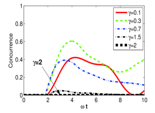
Figure 1: Entanglement generation for different memory times of the noise. A particular initial state is chosen as ψ0=|11⟩.subscriptπœ“0ket11\psi_{0}=\left|11\right\rangle. The curves for different γ𝛾\gamma are marked in the graph. The other parameters are Ο‰A=Ο‰B=0.5​ω,subscriptπœ”π΄subscriptπœ”π΅0.5πœ”\omega_{A}=\omega_{B}=0.5\omega, ΞΊA=ΞΊB=1subscriptπœ…π΄subscriptπœ…π΅1\kappa_{A}=\kappa_{B}=1, Jx​y=0.5.subscript𝐽π‘₯𝑦0.5J_{xy}=0.5.
Refer to caption
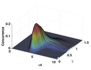
Figure 2: Entanglement generation vs γ𝛾\gamma and t𝑑t. A particular initial state is chosen as ψ0=|11⟩.subscriptπœ“0ket11\psi_{0}=\left|11\right\rangle. The other parameters are Ο‰A=Ο‰B=0.5​ω,subscriptπœ”π΄subscriptπœ”π΅0.5πœ”\omega_{A}=\omega_{B}=0.5\omega, ΞΊ1=ΞΊB=1subscriptπœ…1subscriptπœ…π΅1\kappa_{1}=\kappa_{B}=1, Jx​y=Jz=0.subscript𝐽π‘₯𝑦subscript𝐽𝑧0J_{xy}=J_{z}=0.

With our exact non-Markovian QSD equation (14), we are able to consider the important non-Markovian feature of entanglement generation. For this purpose, we consider the separable state ψ0=|11⟩subscriptπœ“0ket11\psi_{0}=\left|11\right\rangle to show how the environmental memory affects the entanglement generation. It has been known that the entanglement may be generated for a qubit system through coupling qubits to a common bath. However, it is not clear how the environmental correlation times affects entanglement generation. In Fig.Β 1, we plot the entanglement evolution for different parameters of Ξ³,𝛾\gamma, where 1/Ξ³1𝛾1/\gamma gives the memory time of the environment. With this initial state, we can see that when Ξ³β‰₯2𝛾2\gamma\geq 2 (close to the Markov limit for this model), there will be no visible entanglement generated for all times. In fact, it is easy to show that in the Markov limit no entanglement will be generated (i.e. Ξ³β†’βˆžβ†’π›Ύ\gamma\rightarrow\infty) for this special initial state. In addition, it is seen that when the parameter is too small, the entanglement generation becomes less significant shown in our numerical simulations. This shows that the non-Markovian property affects generating entanglement in a subtle way.

We can show that entanglement generation for this special initial state is due to the environmental memory rather than the spin-spin coupling. Interestingly enough, we find that the largest amount of entanglement may be generated if the correlation time of environment is neither too long (γ𝛾\gamma is small) nor too short (γ𝛾\gamma is large). In Fig. 2, we plot the case without coupling between the two spins. The results confirm that entanglement for the two non-interacting qubits is purely generated by environment memory. Our results here have clearly shown that non-Markovian noise can be very useful rather than harmful to the entanglement if the memory times are properly chosen.

III.2 Steady state entanglement
Refer to caption
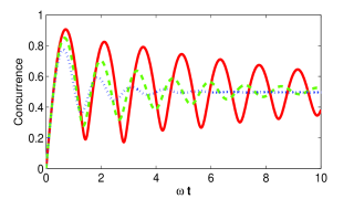
Figure 3: Entanglement generation. The red (solid), green (dashed) and blue (short-dashed) lines represents Ξ³=0.5,𝛾0.5\gamma=0.5, Ξ³=1,𝛾1\gamma=1, Ξ³=2,𝛾2\gamma=2, respectively. The initial state is ψ0=|10⟩.subscriptπœ“0ket10\psi_{0}=\left|10\right\rangle. The other parameters are Ο‰A=Ο‰B=0.5​ω,subscriptπœ”π΄subscriptπœ”π΅0.5πœ”\omega_{A}=\omega_{B}=0.5\omega, Jx​y=0.5,subscript𝐽π‘₯𝑦0.5J_{xy}=0.5, Jz=0.1,subscript𝐽𝑧0.1J_{z}=0.1, ΞΊA=ΞΊB=1.subscriptπœ…π΄subscriptπœ…π΅1\kappa_{A}=\kappa_{B}=1.

Quantum trajectories generated by the non-Markovian QSD equation (3) have many interesting properties. For instance, we can use those quantum trajectories to study the steady state entanglement. In Fig. 3, we plot the entanglement dynamics from a separable initial state ψ0=|10⟩subscriptπœ“0ket10\psi_{0}=\left|10\right\rangle. The numerical results show that the initial pure state evolves into a steady entangled state. In fact, with the help of non-Markovian trajectories, we can show that all the trajectories will localize to the eigenstates of the Lindblad operator L𝐿L and the residual entanglement of the steady state is not zero. Now, let us examine the large t𝑑t behavior of the single trajectories. First, we choose the following four states

|ψ1⟩ketsubscriptπœ“1\displaystyle\left|\psi_{1}\right\rangle =|11⟩,absentket11\displaystyle=\left|11\right\rangle,
|ψ2⟩ketsubscriptπœ“2\displaystyle\left|\psi_{2}\right\rangle =12​(|10⟩+|01⟩),absent12ket10ket01\displaystyle=\frac{1}{\sqrt{2}}(\left|10\right\rangle+\left|01\right\rangle),
|ψ3⟩ketsubscriptπœ“3\displaystyle\left|\psi_{3}\right\rangle =12​(|10βŸ©βˆ’|01⟩),absent12ket10ket01\displaystyle=\frac{1}{\sqrt{2}}(\left|10\right\rangle-\left|01\right\rangle),
|ψ4⟩ketsubscriptπœ“4\displaystyle\left|\psi_{4}\right\rangle =|00⟩.absentket00\displaystyle=\left|00\right\rangle. (15)

which form a complete basis of the Hilbert space. Hence, an arbitrary state can always be written as

|ψ⟩=c1​|ψ1⟩+c2​|ψ2⟩+c3​|ψ3⟩+c4​|ψ4⟩,ketπœ“subscript𝑐1ketsubscriptπœ“1subscript𝑐2ketsubscriptπœ“2subscript𝑐3ketsubscriptπœ“3subscript𝑐4ketsubscriptπœ“4\left|\psi\right\rangle=c_{1}\left|\psi_{1}\right\rangle+c_{2}\left|\psi_{2}\right\rangle+c_{3}\left|\psi_{3}\right\rangle+c_{4}\left|\psi_{4}\right\rangle, (16)

where |c1|2+|c2|2+|c3|2+|c4|2=1.superscriptsubscript𝑐12superscriptsubscript𝑐22superscriptsubscript𝑐32superscriptsubscript𝑐421|c_{1}|^{2}+|c_{2}|^{2}+|c_{3}|^{2}+|c_{4}|^{2}=1.

Substituting Eq. (16) into the QSD Eq. (12), we get the following stochastic differential equations for the coefficients:

βˆ‚βˆ‚t​c1​(t)𝑑subscript𝑐1𝑑\displaystyle\frac{\partial}{\partial t}c_{1}(t) =i​(2​ω+Jz)​c1βˆ’2​F1​(t)​c1βˆ’2​F3​(t)​c1,absent𝑖2πœ”subscript𝐽𝑧subscript𝑐12subscript𝐹1𝑑subscript𝑐12subscript𝐹3𝑑subscript𝑐1\displaystyle=i(2\omega+J_{z})c_{1}-2F_{1}(t)c_{1}-2F_{3}(t)c_{1}, (17)
βˆ‚βˆ‚t​c2​(t)𝑑subscript𝑐2𝑑\displaystyle\frac{\partial}{\partial t}c_{2}(t) =i​(Jx​yβˆ’Jz)​c2+2​ztβˆ—β€‹c1βˆ’2​F1​(t)​c2absent𝑖subscript𝐽π‘₯𝑦subscript𝐽𝑧subscript𝑐22superscriptsubscriptπ‘§π‘‘βˆ—subscript𝑐12subscript𝐹1𝑑subscript𝑐2\displaystyle=i(J_{xy}-J_{z})c_{2}+\sqrt{2}z_{t}^{\ast}c_{1}-2F_{1}(t)c_{2} (18)
+2​F3​(t)​c2βˆ’2​2​F~5​(t,zβˆ—)​c1,2subscript𝐹3𝑑subscript𝑐222subscript~𝐹5𝑑superscriptπ‘§βˆ—subscript𝑐1\displaystyle+2F_{3}(t)c_{2}-2\sqrt{2}\tilde{F}_{5}(t,z^{\ast})c_{1},
βˆ‚βˆ‚t​c3​(t)𝑑subscript𝑐3𝑑\displaystyle\frac{\partial}{\partial t}c_{3}(t) =βˆ’i​(Jx​y+Jz)​c3,absent𝑖subscript𝐽π‘₯𝑦subscript𝐽𝑧subscript𝑐3\displaystyle=-i(J_{xy}+J_{z})c_{3}, (19)
βˆ‚βˆ‚t​c4​(t)𝑑subscript𝑐4𝑑\displaystyle\frac{\partial}{\partial t}c_{4}(t) =i​(Jzβˆ’2​ω)​c4βˆ’2​ztβˆ—β€‹c2.absent𝑖subscript𝐽𝑧2πœ”subscript𝑐42superscriptsubscriptπ‘§π‘‘βˆ—subscript𝑐2\displaystyle=i(J_{z}-2\omega)c_{4}-\sqrt{2}z_{t}^{\ast}c_{2}. (20)

where F~5​(t,zβˆ—)=iβ€‹βˆ«0t𝑑s′​F5​(t,sβ€²)​zsβ€²βˆ—subscript~𝐹5𝑑superscriptπ‘§βˆ—π‘–superscriptsubscript0𝑑differential-dsuperscript𝑠′subscript𝐹5𝑑superscript𝑠′superscriptsubscript𝑧superscriptπ‘ β€²βˆ—\tilde{F}_{5}(t,z^{\ast})=i\int_{0}^{t}ds^{\prime}F_{5}(t,s^{\prime})z_{s^{\prime}}^{\ast}. Here, we assume that the two qubits are identical and symmetric (Ο‰A=Ο‰B,ΞΊA=ΞΊBformulae-sequencesubscriptπœ”π΄subscriptπœ”π΅subscriptπœ…π΄subscriptπœ…π΅\omega_{A}=\omega_{B},\kappa_{A}=\kappa_{B}) for simplicity. The more general case can be dealt with in a similar way. For the initial state ψ0=|10⟩subscriptπœ“0ket10\psi_{0}=|10\rangle, the initial conditions for this set of equations are

c1​(0)subscript𝑐10\displaystyle c_{1}(0) =0,absent0\displaystyle=0, (21)
c2​(0)subscript𝑐20\displaystyle c_{2}(0) =12,absent12\displaystyle=\frac{1}{\sqrt{2}}, (22)
c3​(0)subscript𝑐30\displaystyle c_{3}(0) =12,absent12\displaystyle=\frac{1}{\sqrt{2}}, (23)
c4​(0)subscript𝑐40\displaystyle c_{4}(0) =0.absent0\displaystyle=0. (24)

For the above initial conditions, c1​(t)≑0subscript𝑐1𝑑0c_{1}(t)\equiv 0 at any times, and the steady state solution for c2​(t)subscript𝑐2𝑑c_{2}(t) is simply given by

c2​(∞)=0.subscript𝑐20c_{2}(\infty)=0. (25)

Thus, the large t𝑑t state for a single trajectory will not contain |ψ1⟩ketsubscriptπœ“1\left|\psi_{1}\right\rangle and |ψ2⟩ketsubscriptπœ“2\left|\psi_{2}\right\rangle components, i.e.

|ψfinal⟩=c3​|ψ3⟩+c4​|ψ4⟩.ketsubscriptπœ“finalsubscript𝑐3ketsubscriptπœ“3subscript𝑐4ketsubscriptπœ“4\left|\psi_{\mathrm{final}}\right\rangle=c_{3}\left|\psi_{3}\right\rangle+c_{4}\left|\psi_{4}\right\rangle. (26)

Now, it is clear that all trajectories will always evolve into a sub-space of the Hilbert space spanned by |ψ3⟩ketsubscriptπœ“3\left|\psi_{3}\right\rangle and |ψ4⟩ketsubscriptπœ“4\left|\psi_{4}\right\rangle, which are the eigenstates of the Lindblad operator L=Οƒβˆ’A+Οƒβˆ’B𝐿superscriptsubscript𝜎𝐴superscriptsubscript𝜎𝐡L=\sigma_{-}^{A}+\sigma_{-}^{B}. Moreover, we can easily derive the equations of the motion for the ensemble means of the cross terms. For example, M​[c3βˆ—β€‹c4]𝑀delimited-[]superscriptsubscript𝑐3βˆ—subscript𝑐4M[c_{3}^{\ast}c_{4}] satisfies the following equation:

dd​t​M​[c3βˆ—β€‹c4]=(i​Jx​y+2​i​Jzβˆ’2​i​ω)​M​[c3βˆ—β€‹c4]βˆ’2​M​[ztβˆ—β€‹c3βˆ—β€‹c2].𝑑𝑑𝑑𝑀delimited-[]superscriptsubscript𝑐3βˆ—subscript𝑐4𝑖subscript𝐽π‘₯𝑦2𝑖subscript𝐽𝑧2π‘–πœ”π‘€delimited-[]superscriptsubscript𝑐3βˆ—subscript𝑐42𝑀delimited-[]superscriptsubscriptπ‘§π‘‘βˆ—superscriptsubscript𝑐3βˆ—subscript𝑐2\frac{d}{dt}M[c_{3}^{\ast}c_{4}]=(iJ_{xy}+2iJ_{z}-2i\omega)M[c_{3}^{\ast}c_{4}]-\sqrt{2}M[z_{t}^{\ast}c_{3}^{\ast}c_{2}].

Since c2​(∞)=0subscript𝑐20c_{2}(\infty)=0 in the long-time limit, we have

M​[c3βˆ—β€‹c4]β†’0,M​[c3βˆ—β€‹c4]β†’0.formulae-sequence→𝑀delimited-[]superscriptsubscript𝑐3βˆ—subscript𝑐40→𝑀delimited-[]superscriptsubscript𝑐3βˆ—subscript𝑐40M[c_{3}^{\ast}c_{4}]\rightarrow 0,\,\,M[c_{3}^{\ast}c_{4}]\rightarrow 0. (27)

where t𝑑t is large. Therefore, the density matrix recovered by ρt=M​[|ψt​(zβˆ—)βŸ©β€‹βŸ¨Οˆt​(zβˆ—)|]subscriptπœŒπ‘‘π‘€delimited-[]ketsubscriptπœ“π‘‘superscriptπ‘§βˆ—brasubscriptπœ“π‘‘superscriptπ‘§βˆ—\rho_{t}=M[|\psi_{t}(z^{\ast})\rangle\langle\psi_{t}(z^{\ast})|] will approach to the steady state density matrix in long-time limit:

ρsβ‰ˆ[0000000000M​[c3βˆ—β€‹c3]|tβ†’βˆž0000M​[c4βˆ—β€‹c4]|tβ†’βˆž],subscriptπœŒπ‘ delimited-[]0000000000evaluated-at𝑀delimited-[]superscriptsubscript𝑐3βˆ—subscript𝑐3→𝑑0000evaluated-at𝑀delimited-[]superscriptsubscript𝑐4βˆ—subscript𝑐4→𝑑\rho_{s}\approx\left[\begin{array}[c]{cccc}0&0&0&0\\ 0&0&0&0\\ 0&0&M[c_{3}^{\ast}c_{3}]|_{t\rightarrow\infty}&0\\ 0&0&0&M[c_{4}^{\ast}c_{4}]|_{t\rightarrow\infty}\end{array}\right], (28)

in the basis {|ψ1⟩,\{\left|\psi_{1}\right\rangle, |ψ2⟩,ketsubscriptπœ“2\left|\psi_{2}\right\rangle, |ψ3⟩,ketsubscriptπœ“3\left|\psi_{3}\right\rangle, |ψ4⟩}\left|\psi_{4}\right\rangle\}. The steady state density matrix in the basis {|11⟩,\{\left|11\right\rangle, |10⟩,ket10\left|10\right\rangle, |01⟩,ket01\left|01\right\rangle, |00⟩}\left|00\right\rangle\} is then given by

ρsβ‰ˆ[00000ρ22ρ2300ρ23βˆ—Ο330000ρ44].subscriptπœŒπ‘ delimited-[]00000subscript𝜌22subscript𝜌2300superscriptsubscript𝜌23βˆ—subscript𝜌330000subscript𝜌44\rho_{s}\approx\left[\begin{array}[c]{cccc}0&0&0&0\\ 0&\rho_{22}&\rho_{23}&0\\ 0&\rho_{23}^{\ast}&\rho_{33}&0\\ 0&0&0&\rho_{44}\end{array}\right]. (29)

where ρ22=ρ33=12​M​[c3βˆ—β€‹c3]|tβ†’βˆž,subscript𝜌22subscript𝜌33evaluated-at12𝑀delimited-[]superscriptsubscript𝑐3βˆ—subscript𝑐3→𝑑\rho_{22}=\rho_{33}=\frac{1}{2}M[c_{3}^{\ast}c_{3}]|_{t\rightarrow\infty}, ρ23=βˆ’12​M​[c3βˆ—β€‹c3]|tβ†’βˆžsubscript𝜌23evaluated-at12𝑀delimited-[]superscriptsubscript𝑐3βˆ—subscript𝑐3→𝑑\rho_{23}=-\frac{1}{2}M[c_{3}^{\ast}c_{3}]|_{t\rightarrow\infty} and ρ44=M​[c4βˆ—β€‹c4]|tβ†’βˆžsubscript𝜌44evaluated-at𝑀delimited-[]superscriptsubscript𝑐4βˆ—subscript𝑐4→𝑑\rho_{44}=M[c_{4}^{\ast}c_{4}]|_{t\rightarrow\infty}.

The analytical results shown above can be verified by our numerical simulation as illustrated in the figure 4.
Refer to caption
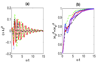
Figure 4: Time evolution of the fluctuation (Δ​L)2superscriptΔ𝐿2(\Delta L)^{2} and the probability |c3|2+|c4|2superscriptsubscript𝑐32superscriptsubscript𝑐42|c_{3}|^{2}+|c_{4}|^{2} for quantum trajectories. Each curve represents a single quantum trajectory. The parameters are Ο‰A=Ο‰B=0.5​ω,subscriptπœ”π΄subscriptπœ”π΅0.5πœ”\omega_{A}=\omega_{B}=0.5\omega, ΞΊA=ΞΊB=1,subscriptπœ…π΄subscriptπœ…π΅1\kappa_{A}=\kappa_{B}=1, Ξ³=1,Jx​y=0.5formulae-sequence𝛾1subscript𝐽π‘₯𝑦0.5\gamma=1,J_{xy}=0.5.

In Fig. 4 (a), we plot the fluctuation of the system Lindblad operator L𝐿L defined as (Δ​L)2=⟨L2βŸ©βˆ’βŸ¨L⟩2superscriptΔ𝐿2delimited-⟨⟩superscript𝐿2superscriptdelimited-⟨⟩𝐿2(\Delta L)^{2}=\left\langle L^{2}\right\rangle-\left\langle L\right\rangle^{2}. It is shown that, as time evolves, the fluctuation of L𝐿LΒ converge to zero in the final steady state for all trajectories. In Fig. 4 (b), we plot the sum of the probabilities of |ψ3⟩ketsubscriptπœ“3\left|\psi_{3}\right\rangle and |ψ4⟩ketsubscriptπœ“4\left|\psi_{4}\right\rangle for a few trajectories. The sum of the probability |c3|2+|c4|2superscriptsubscript𝑐32superscriptsubscript𝑐42|c_{3}|^{2}+|c_{4}|^{2} will always evolve to 111 for any single trajectories which means c1subscript𝑐1c_{1} and c2subscript𝑐2c_{2} are always zero in the final steady state. The numerical results in Fig. 4 simply show that the final state of single trajectories take the form of Eq. (26) as predicted by analytical analysis. In addition, our numerical results show that the final density matrix is approximately given by

ρfinalβ‰ˆ[000000.25βˆ’0.2500βˆ’0.250.2500000.5].subscript𝜌finaldelimited-[]000000.250.25000.250.2500000.5\rho_{\mathrm{final}}\approx\left[\begin{array}[c]{cccc}0&0&0&0\\ 0&0.25&-0.25&0\\ 0&-0.25&0.25&0\\ 0&0&0&0.5\end{array}\right]. (30)

which is also consistent with our prediction in Eq. (29).

It should be noted that such a steady state has be shown to be the stationary solution of the Markov master equation Schneider ; Hope . In our QSD method, it is showed that this state is also the stationary solution of the non-Markovian quantum trajectories. Therefore, the ensemble mean of the quantum trajectories recovers the non-Markovian steady state of the density matrix. It is important to note that our non-Markovian theory does not depend on the existence of the non-Markovian master equation.

Refer to caption
Figure 5: Time evolution of purity for different initial states. The initial states for red (solid), green (dashed), blue (short-dashed) and black (dash-dotted) lines are ψ0=12​(|11⟩+|00⟩),subscriptπœ“012ket11ket00\psi_{0}=\frac{1}{\sqrt{2}}(\left|11\right\rangle+\left|00\right\rangle), ψ0=12​(|01⟩+|10⟩)subscriptπœ“012ket01ket10\psi_{0}=\frac{1}{\sqrt{2}}(\left|01\right\rangle+\left|10\right\rangle), ψ0=|10⟩,subscriptπœ“0ket10\psi_{0}=\left|10\right\rangle, and ψ0=|11⟩subscriptπœ“0ket11\psi_{0}=\left|11\right\rangle, respectively. The other parameters are Ο‰A=Ο‰B=0.5​ω,subscriptπœ”π΄subscriptπœ”π΅0.5πœ”\omega_{A}=\omega_{B}=0.5\omega, ΞΊA=ΞΊB=1,subscriptπœ…π΄subscriptπœ…π΅1\kappa_{A}=\kappa_{B}=1, Ξ³=1,𝛾1\gamma=1, Jx​y=0.7,subscript𝐽π‘₯𝑦0.7J_{xy}=0.7, Jz=0.3.subscript𝐽𝑧0.3J_{z}=0.3.

Finally, we present the time evolution of the purity, defined as P​u​r​i​t​y=t​r​(ρ2)π‘ƒπ‘’π‘Ÿπ‘–π‘‘π‘¦π‘‘π‘Ÿsuperscript𝜌2Purity=tr(\rho^{2}), which determines whether the quantum state is pure or mixed. Specifically, we find the purity of the initial state ψ0=|10⟩,subscriptπœ“0ket10\psi_{0}=\left|10\right\rangle, which evolves into a steady state with some residue entanglement preserved in the final steady state. In Fig. 5, it is validated that the final steady state is a mixed entangled state since the purity is smaller than one at the steady state. The purity is approximately 0.50.50.5 in long time limit, which is consistent with Eq. (30). For all the other three initial states, we will see two qubits will firstly evolve into a mixed (perhaps entangled) state by the coupling interaction, then decay into the final ground state |00⟩ket00\left|00\right\rangle (which is a pure state) due to the dissipative environment.

III.3 Exact versus approximate QSD equations
Refer to caption
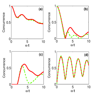
Figure 6: Comparison of the dynamics generated by the approximate O𝑂O operator and the exact O𝑂O operator. The red (solid) curve represents the exact QSD equation, and the green (dashed) curve is for the approximate QSD. (a) (b) (c) and (d) represent four different initial states 12​(|10⟩+|01⟩)12ket10ket01\frac{1}{\sqrt{2}}(\left|10\right\rangle+\left|01\right\rangle), 12​(|11⟩+|00⟩)12ket11ket00\frac{1}{\sqrt{2}}(\left|11\right\rangle+\left|00\right\rangle), |11⟩ket11\left|11\right\rangle and |10⟩ket10\left|10\right\rangle, respectively. The parameters are chosen as Ξ³=0.3𝛾0.3\gamma=0.3, Ο‰A=Ο‰B=0.5​ω,subscriptπœ”π΄subscriptπœ”π΅0.5πœ”\omega_{A}=\omega_{B}=0.5\omega, ΞΊ1=ΞΊB=1subscriptπœ…1subscriptπœ…π΅1\kappa_{1}=\kappa_{B}=1, Jx​y=0.5.subscript𝐽π‘₯𝑦0.5J_{xy}=0.5.

For the coupled two-qubit model, the exact O𝑂O operator contains five terms, as shown in Eq. (8). It is interesting to investigate the perturbative QSD equations based on the exact expression of the O𝑂O operator. For example, we may drop the first order noise-dependent term O5subscript𝑂5O_{5} and only keep the first four terms, i.e. the O𝑂O operator in Eq. (8) is approximately written as

O​(t,s,zβˆ—)𝑂𝑑𝑠superscriptπ‘§βˆ—\displaystyle O(t,s,z^{\ast}) β‰ˆf1​(t,s)​O1+f2​(t,s)​O2absentsubscript𝑓1𝑑𝑠subscript𝑂1subscript𝑓2𝑑𝑠subscript𝑂2\displaystyle\approx f_{1}(t,s)O_{1}+f_{2}(t,s)O_{2}
+f3​(t,s)​O3+f4​(t,s)​O4.subscript𝑓3𝑑𝑠subscript𝑂3subscript𝑓4𝑑𝑠subscript𝑂4\displaystyle+f_{3}(t,s)O_{3}+f_{4}(t,s)O_{4}. (31)

Clearly, the first order term O5subscript𝑂5O_{5} becomes less important when the system is close to the Markov regimes. Also, numerical calculations will be greatly simplified if the first order noise is neglected. In Fig. 6, we have compared the exact time evolution of entanglement and the approximate case without O5subscript𝑂5O_{5}. The numerical result shows that the accuracy of the zeroth order approximation is sensitively dependent on the initial state of the qubits. For the anti-correlated initial states, Fig. 6 (a) and (d) shows that the approximation is extremely good compared with the exact result. On the other hand, for the correlated initial states in case (b) and (c), the noise dependent term tends to smooth out the entanglement curve. In fact, this can be explained by analyzing the QSD Eq. (17-20). If the initial states do not contain ψ1subscriptπœ“1\psi_{1} component, i.e. c1​(0)=⟨ψ0|ψ1⟩=0subscript𝑐10inner-productsubscriptπœ“0subscriptπœ“10c_{1}(0)=\left\langle\psi_{0}|\psi_{1}\right\rangle=0, then c1​(t)subscript𝑐1𝑑c_{1}(t) is always zero during the time evolution. The fifth term of the O𝑂O operator O5=2β€‹Οƒβˆ’Aβ€‹Οƒβˆ’Bsubscript𝑂52superscriptsubscript𝜎𝐴superscriptsubscript𝜎𝐡O_{5}=2\sigma_{-}^{A}\sigma_{-}^{B} will not affect the dynamics of the system, since the coefficient of O5subscript𝑂5O_{5} , i.e. F~5​(t,zβˆ—)subscript~𝐹5𝑑superscriptπ‘§βˆ—\tilde{F}_{5}(t,z^{\ast}), is always associated with c1​(t)subscript𝑐1𝑑c_{1}(t). This observation explains our results plotted in Fig.Β 6. As shown in Fig.Β 6, the noiseless approximation (setting O5=0subscript𝑂50O_{5}=0) gives extremely good results for the two initial states which do not contain |11⟩ket11\left|11\right\rangle component. Our simple analysis here has already shown the complexity level of the approximate QSD equations arising from the noise expansion of the O𝑂O operator. More in-depth study on the approximate QSD equations will be presented elsewhere.

IV Conclusion

In conclusion, the central aim of this paper is to develop a time-local theory of non-Markovian quantum state diffusion for a model consisting of two interacting qubits – a model that is of interest for both quantum information processing and quantum optics. As an application, we used the non-Markovian quantum trajectory to analyze the entanglement evolution of the qubit system for several parameters ranging from strongly non-Markovian to Markov regimes. Our results also showed explicitly how the environmental memory generates the entanglement of the qubit system. With the non-Markovian QSD equation, we further studied the entanglement evolution and the steady entangled state for the QSD equation. Our time-local QSD approach may be extended to multiple qubit systems, this will be the topic for a future publication.

ACKNOWLEDGMENTS

We would like to thank Professors J. H. Eberly, B. L. Hu and W. T. Strunz for many interesting conversations and acknowledge support by grants from DARPA QuEST HR0011-09-1-0008, the NSF PHY-0925174. Part of this work was done while T.Y. enjoyed the hospitality of the Kavli Institute for Theoretical Physics China, Beijing.

References

  • (1) C. W. Gardiner and P. Zoller, Quantum Noise (Springer-Verlag, 2004).
  • (2) H. P. Breuer and F. Petruccione, Theory of Open Quantum Systems (Oxford, New York, 2002).
  • (3) M. A. Nielsen and I. L. Chuang 2000 Quantum computation and quantum information (Cambridge University press, Cambridge, England, 2000).
  • (4) H. Carmichael, An Open System Approach to Quantum Optics (Springer, Berlin, 1994).
  • (5) J. Dalibard, Y. Castin, and K. MΓΈlmer, Phys. Rev. Lett. 68, 580 (1992).
  • (6) N. Gisin, I. C. Percival, J. Phys. A 25, 5677 (1992); ibid. 26, 2233 (1993).
  • (7) M. B. Plenio, P. L. Knight, Rev. Mod. Phys. 70, 101 (1998).
  • (8) J. Xu et al., Phys. Rev. Lett. 104, 100502 (2010).
  • (9) B. Bellomo, R. LoFranco, G. Compagno, Phys. Rev. Lett. 99, 160502 (2007).
  • (10) T. Yu, J. H. Eberly, Opt.Β Commun. 283, 676 (2010).
  • (11) N. Vats, S. John, Phys. Rev. A 58, 4168 (1998).
  • (12) B. L. Hu, J. P. Paz, and Y. Zhang, Phys.Β Rev. D 45, 2843 (1992).
  • (13) J. H. An, W. M. Zhang, Phys.Β Rev. A 76, 042127 (2007); M. W. Y. Tu, W. M. Zhang, Phys.Β Rev. B 78, 235311 (2008).
  • (14) J. S. Jin, X. Zheng and Y. J. Yan, J. Chem. Phys. 128, 234703 (2008).
  • (15) R. X. Xu, F. Cui, X. Q. Li, Y. Mo, and Y. J. Yan, J. Chem. Phys. 122, 041103 (2005).
  • (16) J. S. Shao, Chem. Phys. 322, 187 (2006).
  • (17) J. Tan, T. H. Kyaw, Y. Yeo, Phys. Rev. A 81, 062119 (2010).
  • (18) L. DiΓ³si, N. Gisin, and W. T. Strunz, Phys. Rev. A 58, 1699 (1998); see also W. T. Strunz, L. DiΓ³si, and N. Gisin, Phys. Rev. Lett. 82, 1801 (1999).
  • (19) T. Yu, L. Diosi, N. Gisin, and W. T. Strunz, Phys. Rev. A 60, 91 (1999).
  • (20) W. T. Strunz, Chem. Phys. 268, 237 (2001).
  • (21) W. T. Strunz, T. Yu, Phys. Rev. A 69, 052115 (2004).
  • (22) S. Nakajima, Prog. Theor. Phys. 20, 948 (1958).
  • (23) R. W. Zwanzig, J. Chem. Phys. 33, 1338 (1961).
  • (24) F. Haake, Statistical Treatment of Open Systems by Generalized Master Equations, Springer Tracts in Mod. Phys. 66, 98 (1973).
  • (25) J. Jing, T. Yu, Phys. Rev. Lett. 105, 240403 (2010).
  • (26) B.Β Corn, J. Jing, T. Yu, arXiv:1105.1358 (to be published).
  • (27) M. C. Arnesen, S. Bose, V. Vedral, Phys. Rev. Lett. 87, 017901 (2001).
  • (28) G. L. Kamta, A. F. Starace, Phys. Rev. Lett. 88, 107901 (2002).
  • (29) L. Zhou, H. S. Song, Y. Q. Guo, C. Li, Phys. Rev. A 68, 024301 (2003).
  • (30) M. J. Hartmann, F. G. S. L. BrandΓ£o, M. B. Plenio, Phys. Rev. Lett. 99, 160501 (2007).
  • (31) T. Yu, J. H. Eberly, Phys.Β Rev. B 66, 193306 (2002).
  • (32) W. DΓΌr, H. J. Briegel, Phys. Rev. Lett. 92, 180403 (2004).
  • (33) T. Yu, J. H. Eberly, Phys. Rev. Lett. 93, 140404 (2004); Phys.Β Rev.Β Lett. 97, 140403 (2006); T. Yu, J. H. Eberly, Science 323, 598 (2009).
  • (34) A. R. R. Carvalho, F. Mintert, A. Buchleitner, Phys. Rev. Lett. 93, 230501 (2004).
  • (35) F. Mintert, A. R. R. Carvalho, M. KuΕ›, A. Buchleitner, Phys. Rep. 415, 207 (2005).
  • (36) Z. Ficek, R. Tanas, Phys. Rev. A 74, 024304 (2006); S. Natali, Z. Ficek, Phys.Β Rev. A 75, 042307 (2007).
  • (37) J. Helm, W. T. Strunz Phys. Rev. A 80, 042108 (2009); Phys. Rev. A 81, 042314 (2010).
  • (38) Z. Sun, X. G. Wang, and C. P. Sun, Phys. Rev. A 75, 062312 (2007).
  • (39) Q. Ai, Y. Li, G. L. Long, and C. P. Sun, Euro. Phys. J. D 48, 293 (2008);
  • (40) W. K. Wootters, Phys. Rev. Lett. 80, 2245 (1998).
  • (41) S. Schneider, G. J. Milburn, Phys. Rev. A 65, 042107 (2002).
  • (42) A. R. R. Carvalho, J. J. Hope, Phys, Rev.Β A 76 010301(R) (2007).