Emission Patterns and Light Curves of Gamma-Rays in the Pulsar Magnetosphere with a Current-Induced Magnetic Field

Abstract

We study the emission patterns and light curves of gamma-rays in the pulsar magnetosphere with a current-induced magnetic field perturbation. Based on the solution of a static dipole with the magnetic field induced by some currents (perturbation field), we derive the solutions of a static as well as a retarded dipole with the perturbation field in the Cartesian coordinates. The static (retarded) magnetic field can be expressed as the sum of pure static (retarded) dipolar magnetic field and the static (retarded) perturbation field. We use the solution of the retarded magnetic field to investigate the influence of the perturbation field on the emission patterns and light curves, and we apply the perturbed solutions to calculate the gamma-ray light curves for the case of the Vela pulsar. We find out that the perturbation field induced by the currents will change the emission patterns and then light curves of gamma-rays, especially for a larger perturbation field. Our results indicate that the perturbation field created by the outward-flowing (inward-flowing) electrons (positrons) can decrease the rotation effect on the magnetosphere and makes emission pattern appear to be more smooth relative to that of the pure retarded dipole, but the perturbation field created by the outward-flowing (inward-flowing) positrons (electrons) can make the emission pattern less smooth.

1 Introduction

Since pulsed gamma-ray emission from a large number of pulsars by the Large Area Telescope (LAT) on the Fermi Gamma-Ray Space Telescope have been discovered (Abdo et al., 2010), much information are available for constraining pulsar magnetosphere geometry. Rotation-powered pulsars are widely believed to have their magnetospheres in which charged particles are accelerated to relativistic energy and generate multiband spectra of pulsed emission. In order to simulate pulsar magnetosphere, various approximations have been proposed. Vacuum magnetosphere model is analytic model for the electromagnetic field of a rotating magnetic dipole (Deutsch, 1955), but it is not an appropriate physical model of an active pulsar magnetosphere filled with charges and currents. Force-free magnetosphere is probably a closer approximation to a real pulsar than the vacuum solution, however it is not a truly self-consistent model since the production of pair plasma requires particle acceleration and thus a break down of force-free conditions in some regions of the magnetosphere. At present, there are two kinds of three dimensional (3D) emission models: one is based on the geometrical consideration such as two pole caustic (TPC) model in the frame of a retarded dipole (e.g., Dyks & Rudak, 2003; Dyks et al., 2004; Fang & Zhang, 2010) and annular gap (AG) model in the frame of free-force approximation (Bai & Spitkovsky, 2010a); another is based on both physical and geometrical consideration such as slot gap (SG) (Harding et al., 2008) and outer gap models (e.g., Romani & Yadigaroglu, I.-A., 1995; Cheng et al., 2000; Zhang & Cheng, 2000, 2001, 2002; Tang et al., 2008; Zhang & Li, 2009; Watters et al., 2009; Li & Zhang, 2010; Wang et al., 2011).

How we can describe a pulsar magnetosphere filled with charges and currents? Since the currents will induce magnetic field perturbation, resulting to a distorted magnetic field relative to dipole field, Muslimov & Harding (2009) described an approximate perturbation field for a pair-starved current flow in the open zone in the frame of static magnetic dipole. In their treatment, the magnetic field is described as $\textbf{B}=\textbf{B}^{\rm(d)}+\epsilon\textbf{B}^{(1)}$, where $\textbf{B}^{\rm(d)}$ is a pure dipole magnetic field anchored into the neutron star (NS), $\epsilon$ is the perturbation amplitude which determines the strength of the $\textbf{B}^{(1)}$ relative to the dipole one , and $\textbf{B}^{(1)}$ is the magnetic field generated by the self-consistent electric currents in the domain of the magnetosphere with open field lines, where a singularity exists on the symmetry axis (details see in Muslimov & Harding (2009)). However, although basic features of the pulsar magnetosphere in a static dipolar magnetic field approximation can be understood, it is more realistic that the magnetosphere be approximated as a rotating inclined magnetic dipole. The magnetic field lines of a rotating inclined dipole are especially different from those of a static dipole for large inclination angles. Romani & Watters (2010) investigated the magnetic field structure with a current-induced field in the frame of the retarded magnetic dipole. To apply the solution of Muslimov & Harding (2009) to the retarded dipole, Romani & Watters (2010) made following treatments: (1) shifted the magnetic axis ($r$, $\theta_{\rm B}=0$, $\phi_{\rm B}$) to match that of the swept back dipole (i.e. mapped the magnetic axis line onto the swept back curve) and (2) exponentially tapered the singularity appeared on the symmetry axis so that the field lines can be integrated to determine the last closed field line surface. Obviously, such a treatment method is highly simplified.

In this paper, we study the emission patterns and light curves in the pulsar magnetosphere with a current-induced magnetic field perturbation. We derive the analytic solution of the retarded magnetic field with a current-induced magnetic field; this solution is that of Muslimov & Harding (2009) when rotating effects are ignored. We find that our calculated results are different from those given by Romani & Watters (2010), for example open zone boundary (polar cap) foot-points. Using such a solution, we calculate emission patterns and light curves for the Vela pulsar with different inclination angels in the frame of two pole outer gap model, where a self-consistent treatment is that both simulation of the magnetosphere and relativistic effects are performed in the inertial observer’s frame (IOF) (e.g., Takata et al., 2007; Bai & Spitkovsky, 2010b). The paper is organized as follows. In §2, the solution of the magnetic field structure with current-induced magnetic field is given. Various emission patterns and light curves are calculated in §3. Finally, a brief discussion and conclusions are given in §4.

2 Magnetic Field Structure

In a pulsar magnetosphere, radiating charges accelerated in gaps will create some currents in the open zone. If gap-closing pair front produce densities comparable to the co-rotation value for at least some of the open field lines, this current will induce a magnetic field (e.g., Muslimov & Harding, 2009; Romani & Watters, 2010). For a static dipole, the local magnetic field can be described as (Muslimov & Harding, 2009)

$$\textbf{B}=\textbf{B}^{\rm(d)}+\epsilon\textbf{B}^{(1)}\;,$$ (1)

where $\textbf{B}^{\rm(d)}$ is the pure dipole magnetic field and is given by

$$\textbf{B}^{\rm(d)}=\frac{1}{r^{3}}\left[3({\bf m}\cdot{\bf\hat{r}}){\bf\hat{r}}-{\bf m}\right]\;,$$ (2)

where $\bf m$ is the magnetic moment and its three components in Cartesian coordinates can be expressed as (the derivation is shown in Appendix A)

$$m_{x} = \frac{r}{2}\left[(3x^{2}-2r^{2})B^{\rm(d)}_{x}+3xyB^{\rm(d)}_{y}+3xzB^{\rm(d)}_{z}\right]$$

$$m_{y} = \frac{r}{2}\left[3yxB^{\rm(d)}_{x}+(3y^{2}-2r^{2})B^{\rm(d)}_{y}+yzB^{\rm(d)}_{z}\right]$$ (3)

$$m_{z} = \frac{r}{2}\left[3xzB^{\rm(d)}_{x}+3yzB^{\rm(d)}_{y}+(3z^{2}-2r^{2})B^{\rm(d)}_{z}\right]\;,$$

where $r=\sqrt{x^{2}+y^{2}+z^{2}}$, and $B^{\rm(d)}_{x}$, $B^{\rm(d)}_{y}$, and $B^{\rm(d)}_{z}$ are three components of the magnetic field given by Eq. (2). In Eq. (1), $\epsilon$ is the perturbation amplitude, and $\textbf{B}^{(1)}$ is the magnetic field generated by the self-consistent electric currents in the domain of the magnetosphere with open field lines. After introducing cosine of the angle between the neutron star(NS) rotation axis and radius-vector of a given point $s=\cos\alpha\cos\theta+\sin\alpha\sin\theta\cos\phi$ and its derivatives over $\theta$ and $\phi$, Muslimov & Harding (2009) derived the analytic expressions of Eq. (1) in magnetic polar coordinates for the static dipole, where $s=1$ determines the symmetry axis in magnetic coordinates which is the NS rotation axis. In Appendix A, we change expressions ($B_{r}$, $B_{\theta}$, $B_{\phi}$) of Eq. (1) in magnetic polar coordinates to those ($B_{x}$, $B_{y}$, $B_{z}$) in Cartesian coordinates, and then give three components of the magnetic moment $\bf{m^{\prime}}$ in which the magnetic field is given by Eq. (1) (i.e. the perturbation field is included) by changing ($B^{\rm(d)}_{x}$, $B^{\rm(d)}_{y}$, $B^{\rm(d)}_{z}$) to ($B_{x}$, $B_{y}$, $B_{z}$) in Eq. (3). In such a treatment, the magnetic moment $\bf{m}$ in the pure dipole magnetic field changes to $\bf{m^{\prime}}$ in the magnetic field given by Eq. (1). We call $\bf{m^{\prime}}$ as an effective magnetic moment. The difference between $\bf{m}$ and $\bf{m^{\prime}}$ depends on the perturbation amplitude $\epsilon$, $\delta\bf{m}=|\bf{m}-\bf{m^{\prime}}|=0$ when $\epsilon=0$.

Since the perturbation field becomes singular along the rotation axis where $s\rightarrow\pm 1$, Romani & Watters (2010) exponentially tapered this singularity ($\propto 1-\exp[(|s|-1)/\sigma_{s}]$, with $\sigma_{s}=0.25$) so that the field lines can be integrated to determine the last closed field line surface. Here we will use this method.

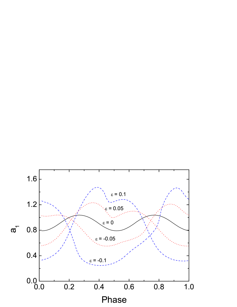
Figure 1: Changes of open zone boundary (polar cap) foot-points with phase for the $\alpha=70^{\circ}$ static dipole with current-induced perturbations $\epsilon=0,\pm 0.05$, and $\pm 0.1$. The Vela pulsar’s parameters are used.

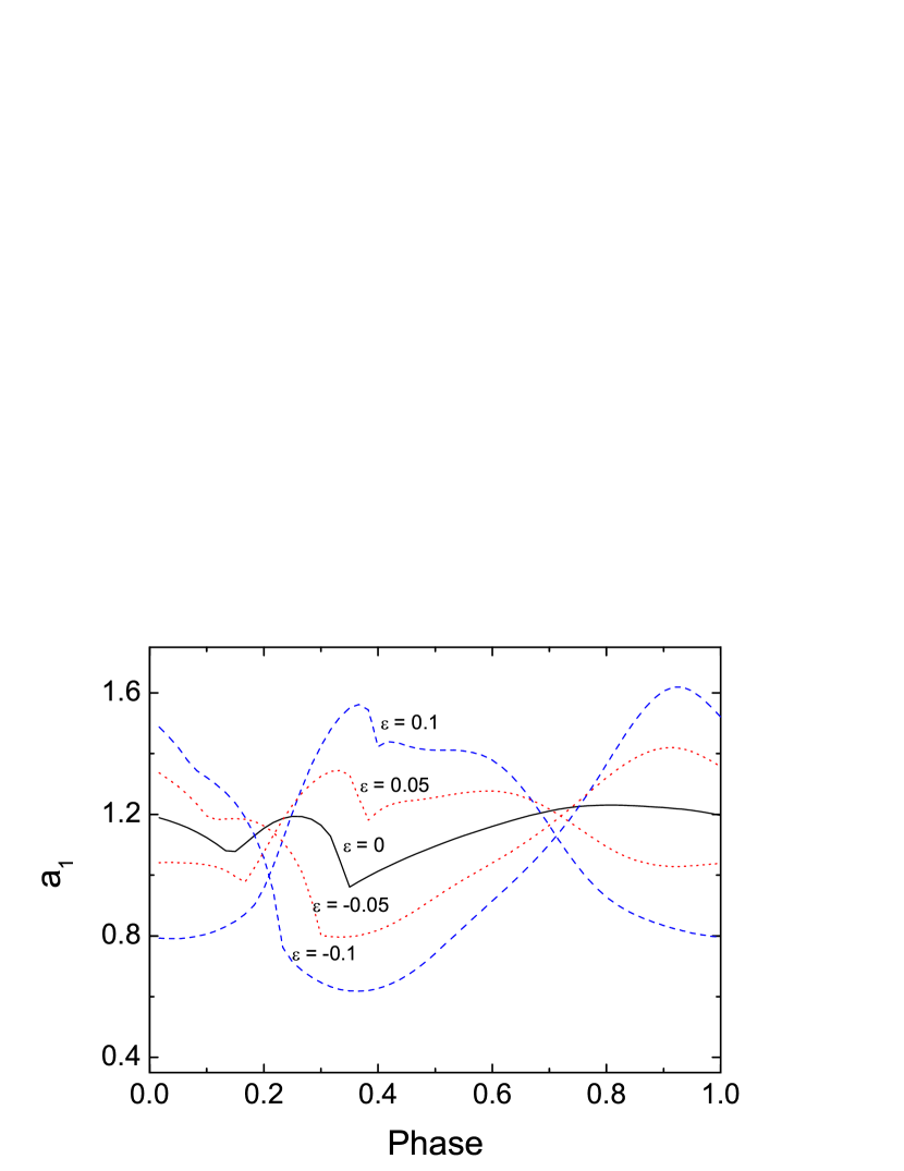
Figure 2: Changes of open zone boundary (polar cap) foot-points with phase for the $\alpha=70^{\circ}$ retarded dipole with current-induced perturbations $\epsilon=0,\pm 0.05$, and $\pm 0.1$. The Vela pulsar’s parameters are used.

Figure 3: Changes of open zone boundary (polar cap) foot-points with phase for the $\alpha=70^{\circ}$ retarded dipole with $\epsilon=0$ for the periods of Crab, Vela, and Geminga pulsars.

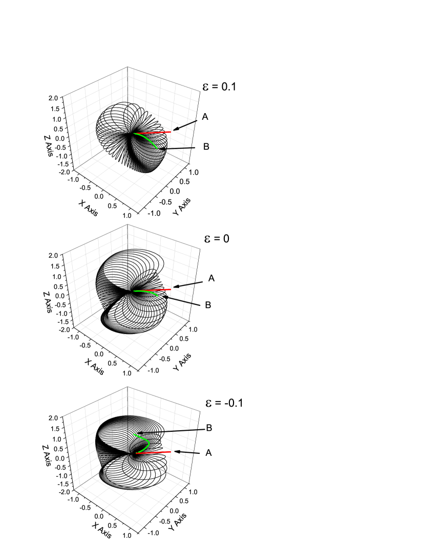
Figure 4: A three-dimensional view of last closed field lines for a retarded dipole with or without the perturbation field inclined to the rotation axis with angle $\alpha=50^{\circ}$ for Vela pulsar. The magnetic field is given by Eq. (5). The panels from top to bottom represent that the cases of $\epsilon=0.1$, $\epsilon=0.0$, and $\epsilon=-0.1$. For each panel, the thick red line marked by A represents the magnetic axis of pure static dipole, and the thick green curved line marked by B represents the magnetic axis of the retarded magnetic field given by Eq.(5).

The structure of the magnetosphere can still only be described by a specific features such as the last closed field lines. The footprints of the last closed field lines on the stellar surface define the polar cap shape. In the static approximation, the polar cap shape is a circle with radius of $R_{\rm pc}=R_{0}(R_{0}/R_{\rm L})^{1/2}$ for an aligned dipole, where $R_{\rm L}\equiv c\Omega^{-1}$ is the light cylinder radius, and $R_{0}$ is radius of the neutron star. we define the initial polar cap’s edge using $(x_{0},y_{0},z_{0})=[R_{\rm pc}{\rm cos}(\phi_{\rm p}),R_{\rm pc}{\rm sin}(\phi_{\rm p}),(R_{0}^{2}-R_{\rm pc}^{2})\ ],$ where $\phi_{\rm p}$ is the azimuthal angle about the magnetic axis. Then we try to find the scaling factors $a_{0}$ such that $(x_{0}^{\prime},y_{0}^{\prime},z_{0}^{\prime})=[a_{0}x_{0},a_{0}y_{0},(R_{0}^{2}-a_{0}^{2}R_{\rm p}^{2})^{1/2}\ ]$ by using the Runge-Kutta method (Zhang & Cheng, 2001). Next we define another scaling factor $a_{1}$ to denote the footprints of the open field lines as $(x,y,z)=(a_{1}x_{0}^{\prime},a_{1}y_{0}^{\prime},[R_{0}^{2}-(x^{2}+y^{2})]^{1/2})$. As an example, we show the variation of open zone boundary (polar cap) foot-points with phase for the $\alpha=70^{\circ}$ static dipole with current-induced perturbations $\epsilon=0,\pm 0.05$, and $\pm 0.1$ for Vela pulsar parameters (i.e. its period is $P=0.0893$ s and surface magnetic field is $B=3.3\times 10^{12}$ G) in Fig. 1. It can be seen that the open zone boundary appears two symmetric peaks if the current-induced B perturbation is not included (i.e. $\epsilon=0$). However, such a symmetry breaks when the current-induced B perturbations is included (i.e. $\epsilon\neq 0$).

For an inclined dipole of constant magnitude, rotating with angular frequency $\Omega$ about the $\hat{z}$-axis in which the magnetic field consists of pure retarded dipolar magnetic field and perturbation field, the magnetic moment is

$$\bf{m}^{{}^{\prime}r}=\bf{m}^{r}+\epsilon\bf{m}^{r}_{p}\;,$$ (4)

where $\bf{m}^{r}$ and $\bf{m}^{r}_{p}$ are the magnetic moments of pure retarded dipolar magnetic field $\bf{B}^{r}$ and perturbation magnetic field $\bf{B}^{r}_{p}$, respectively and the expression are given in Appendix B. In such a case, the magnetic field is

$$\bf{B}^{{}^{\prime}r}=\bf{B}^{r}+\epsilon\bf{B}^{r}_{p}\;,$$ (5)

where the expressions of $\bf{B}^{r}$ and $\bf{B}^{r}_{p}$ are given in Appendix B.

In Fig. 2, we show the variation of open zone boundary foot-points with phase for the $\alpha=70^{\circ}$ retarded dipole with current-induced perturbations $\epsilon=0,\pm 0.05$, and $\pm 0.1$ for comparison with the results of Romani & Watters (2010). Since the rotating effect in the retarded dipole is included, two symmetric peaks disappear even the current-induced B perturbation is not included (i.e. $\epsilon=0$). This result with $\epsilon=0$ is consistent with that of Romani & Watters (2010) (see their top panel of Fig. 2), but there is a small difference between our result and the result of Romani & Watters (2010). In fact, the shape of the open zone boundary foot-points depends on not only the magnetic inclination angle but also the pulsar’s period, we show the shapes for the periods of Crab, Vela, and Geminga with $\alpha=70^{\circ}$ in Fig. 3 to account for this fact. Moreover, the cylindrical radius $r_{\perp}=1.2R_{\rm L}=1.2c/\Omega$ was used in Romani & Watters (2010), but $r_{\perp}=R_{\rm L}$ is used in our treatment, leading to the difference. With increasing B perturbation (i.e. increasing $\epsilon$), open zone boundary is significantly different from that with $\epsilon=0$, as shown in Fig 2. More importantly, for the singularity in the pair-starved field of Muslimov & Harding (2009), we use the smooth method of Romani & Watters (2010) to deal with it in static dipole field (see Fig. 1), so this singularity does not exist in retarded dipole field. However, Romani & Watters (2010) took the solution of Muslimov & Harding (2009), and shifted the magnetic axis to match the retarded dipole by simply mapped the magnetic axis line onto the swept back curve. Therefore, our results with $\epsilon\neq 0$ are very different from those given by Romani & Watters (2010). Physically, the perturbation fields with $\epsilon<0$ and $\epsilon>0$ should have opposite roles on pure retarded dipole field, our results show this property, so we believe that our results are reasonable.

In the retarded dipole, the magnetic axis is curved relative to that of pure static dipole. In Fig. 4, we show a three-dimensional view of last closed field lines for a retarded dipole with or without the perturbation field inclined to the rotation axis with angle $\alpha=50^{\circ}$, where the thick red line marked by A represents the magnetic axis of pure static dipole, and the thick green curved line marked by B represents the magnetic axis of the retarded dipole with the perturbation field ($\epsilon\neq 0$). It can be seen that the perturbation field has an important role in both the shape of the last closed field lines and the magnetic axis. For example, when $\epsilon>0$, the shape of the last closed field lines becomes more smooth and the magnetic axis is more curved on the side of the magnetic axis of pure retarded dipole (see top panel of Fig. 4).

3 Emission Patterns and Light Curves

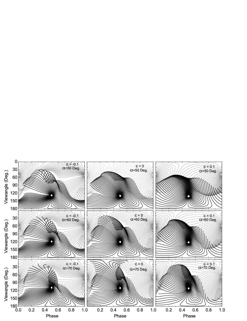
Figure 5: Emission projections onto the $(\zeta,\Phi)$-plane for various magnetic inclination angles and for $\epsilon=0.1$, 0, and -0.1. The black lines represent the emission from one pole and the grey lines represent the emission from another pole. Vela pulsar parameters are used.

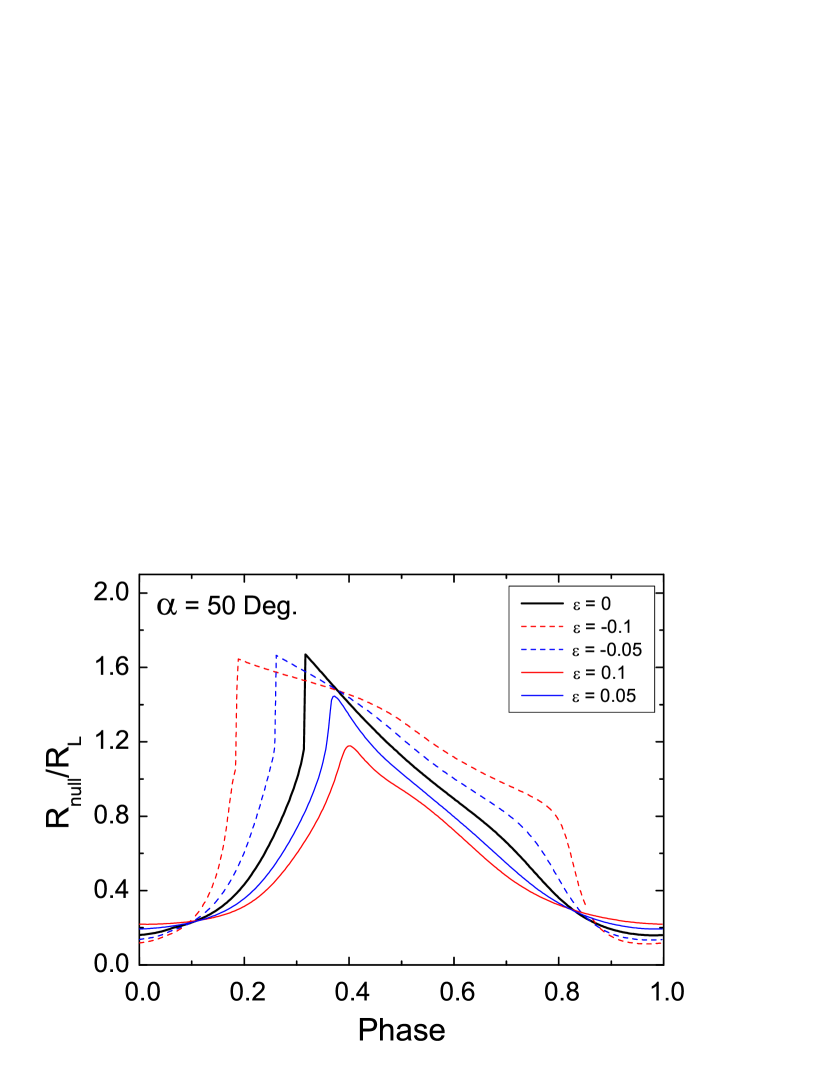
Figure 6: Radial distances to the null charge surface for the last open field lines for $\alpha=50^{\circ}$ and different values of $\epsilon$. The Vela pulsar’s parameters are used.

Figure 7: Light Curves for different magnetic inclinations, view angles, and $\epsilon$. Panel A: $\alpha=50^{\circ}$, $\zeta=60^{\circ}$, $75^{\circ}$, $90^{\circ}$, and $\epsilon=-0.1$, 0, 0.1. Panel B: $\alpha=60^{\circ}$, $\zeta=60^{\circ}$, $75^{\circ}$, $90^{\circ}$, and $\epsilon=-0.1$, 0, 0.1. Panel C: $\alpha=70^{\circ}$, $\zeta=60^{\circ}$, $75^{\circ}$, $90^{\circ}$, and $\epsilon=-0.1$, 0, 0.1. Both outward emission from one pole and inward emission from another pole are included and the azimuthal range of outer gaps is limited by using the method of Fang & Zhang (2010). The Vela pulsar’s parameters are used.

In order to determine photon emission from the outer gaps, 3D pulsar’s magnetosphere should be simulated and relativistic effects including photon abberation and time-of-flight phase shifts need to be taken into account. The geometry of the photon emission is usually expressed as $(\zeta,\Phi)$, where $\zeta$ is the polar angle from the rotation axis and $\Phi$ is the phase of rotation of the star. Here we consider the photon emissions from two poles of pulsar magnetosphere and the photon emission geometries in the inertial observer’s frame (IOF).

The particle motion in the IOF is described by (Takata et al., 2007)

$${\bf n}=[\beta_{0}\cos\varphi(r)]{\bf b}+[\beta_{0}{\rm sin}\varphi(r)]{\bf b_{\bot}}+\beta_{\rm co}{\bf e_{\phi}},$$ (6)

where $\varphi(r)$ is the pitch angle. The third term represent corotation with the star, $\beta_{\rm co}=\rho\Omega/c.$ The quantity $\beta_{0}$ at each point is determined by the condition that ${\bf|n|}=1$. The unit vector ${\bf b_{\bot}}$ perpendicular to the magnetic field line is

$${\bf b_{\bot}}\equiv\pm[({\rm cos}\delta\phi){\bf k}+({\rm sin}\delta\phi){\bf k\times b}],$$ (7)

where $\pm$ corresponds to the gyration of the positrons (+) or electrons (-), $\delta\phi$ refers to the phase of the gyration, and ${\bf k=(b\cdot\nabla)b/|(b\cdot\nabla)b|}$ represents the unit vector of the curvature of the magnetic field line. Therefore, the emission direction $(\zeta,\Phi)$ in the IOF is

$${\rm cos}\zeta=n_{z},$$ (8)

and

$$\Phi=-\Phi_{n}-{\bf r\cdot n},$$ (9)

where $-\Phi_{n}$ is the azimuthal angle of the emission direction, and r is the emitting location in units of the light radius.

We now consider the emission patterns and the examples are shown in Fig. 5. In this figure, the emission patterns with $\epsilon=0.1$, 0, and -0.1 for $\alpha=50^{\circ}$, $60^{\circ}$, and $70^{\circ}$ are given. For the magnetic field with the perturbation field, the emission patterns is different from those for the pure retarded dipole. The emission pattern for $\epsilon>0$ appears to be more smooth relative to that of the pure retarded dipole, but the emission pattern for $\epsilon<0$ is less smooth (see Fig. 5). Note that the differences depend on the value of $\epsilon$.

Before calculating the light curves, we consider the change of the null charge surface with the phase. In the two-pole caustic model of Dyks & Rudak (2003), photons are emitted uniformly in the gap, and the gap extending from the star surface to high altitudes is confined to the last open field lines. Fang & Zhang (2010) made a revised version of the two-pole caustic model, they pointed out that although acceleration gaps can extend from the star surface to the light cylinder along near the last open field lines, the extension of the gaps along the azimuthal direction is limited because of photon-photon pair production process. In such gaps, high-energy photons are emitted uniformly and tangentially to the field lines but cannot be efficiently produced along these field lines where the distances to the null charge surface are larger than $\sim 0.9$ times of the distance of the light cylinder. In Fig. 6, we show the changes of the null charge surface with the phase for $\alpha=50^{\circ}$ but different values of $\epsilon$. It can be seen from this figure that there are substantially difference between the null charge surfaces of the pure retarded dipole with and without the perturbation field, and the difference becomes larger when $\epsilon$ increases.

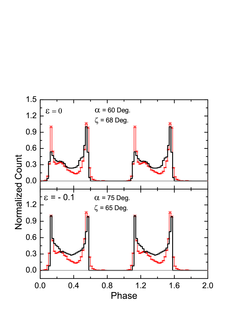
Figure 8: Comparison of light curves (black solid lines) predicted in two pole outer gap model with observed light curve (red lines with error bars) in energy region from 0.1 GeV to 10 GeV of Vela pulsar (Abdo et al., 2009). The predicted light curves in upper and bottom panels are calculated in the retarded field without any perturbation and with a perturbation of $\epsilon=-0.1$, respectively. Note that the predicted light curves come mainly from the contribution of one pole since the contribution (grey lines) of another pole can be neglected when the values of $\alpha$ and $\zeta$ listed in the figure are used.

In calculating the light curves, we use the method given by Fang & Zhang (2010), i.e. the emission region is limited in the range of $r_{\rm null}/R_{\rm L}\leq 0.9$ and $\rho_{\rm max}/R_{\rm L}=0.95$, where $\rho_{\rm max}$ is the distance from the rotation axis. On the other hand, we use the method given by Dyks & Rudak (2003) to smooth the light curves, i.e. the model light curve was calculated for electrons distributed evenly along the polar cap rim; the density profile across the rim was assumed to be the Gaussian function $f(\theta_{\rm m})$ symmetrical about $\theta_{\rm m}=\theta_{\rm pc}$, with $\sigma=0.025\theta_{\rm pc}$, where $\theta_{\rm m}$ is the magnetic colatitude of magnetic field lines’ footprints at the star surface, and $\theta_{\rm pc}\approx(r_{\rm ns}/r_{\rm lc})^{1/2}$ is the magnetic colatitude of the rim. We show the light curves in different magnetic inclinations and view angles for $\epsilon=-0.1$, 0.0, and 0.1 in Fig. 7, where we have assumed that the inner boundary of the outer gap is located on the stellar surface. It can be seen that the change of the light curves with $\epsilon\neq 0$ is remarkable relative to those with $\epsilon=0$, particularly for larger value of $\epsilon$. Compared to the light curves with $\epsilon=0$, the light curves with $\epsilon\neq 0$ have following features: (1) peak shapes is changed although the peak separations are roughly the same, and (2) the light curves with $\epsilon>0$ are more smoothing but those with $\epsilon<0$ become more complicated. In Fig. 8, we show the light curves predicted in the frame of two pole outer gap model and compare them with observed one of energy region from 0.1 GeV to 10 GeV of Vela pulsar (Abdo et al., 2009). The predicted light curve in the upper panel is calculated in the retarded field without any perturbation, while the lower panel is calculated in the retarded field with a perturbation of $\epsilon=-0.1$. In our calculations for Fig.8, the inner boundary of the outer gap is assumed to be the null charge surface, the predicted light curves are mainly produced by the emission of one pole although the contributions of two poles are included when the values of $\alpha$ and $\zeta$ listed in the figure are used. Note that the light curves predicted in Romani & Watters (2010) are based on their one pole outer model given by Romani (1996), we can reproduce their result with $\epsilon=0$ in this one pole outer gap model when we used the parameters (i.e. $\alpha=72^{\circ}$ and $\xi=64^{\circ}$) listed in Fig. 5 of Romani & Watters (2010). Comparing our results with their results we reached the same conclusion, i.e. that the light curve with $\epsilon<0$ is more consistent with the observed one for the Vela pulsar.

4 Discussion and Conclusions

Since some currents in the open zone will be created by the radiating charges accelerated in the gaps and the currents will induce the magnetic field (e.g., Muslimov & Harding, 2009; Romani & Watters, 2010), it is important to study the structure of the magnetic field with the perturbation field, emission patterns, and light curves in pulsar magnetosphere. In this paper, we derive the solution of the static (retarded) magnetic field with the perturbation field in the Cartesian coordinates, which can be expressed as the sum of pure static (retarded) dipolar magnetic field and the perturbation field in in the Cartesian coordinates. We have confirmed the reliability of our results by using the solution of the static magnetic field with the perturbation field (see Fig. 1), and then we have used the solution of the retarded magnetic field with the perturbation field to investigate the emission patterns and light curves in the pulsar magnetosphere (the parameters of the Vela pulsar are used). Our results show that the photon emission pattern and light curves for the retarded magnetic field with the perturbation field are changed with respective to those for pure retarded dipolar magnetic field (see Figs. 5 and 7).

Romani & Watters (2010) have studied the emission patterns and light curves of the retarded magnetic field with the perturbation field by using a highly simplified method. However, our method is totally different from their method and the results obtained for these two methods are different (see Figs. 2 and 8). It should be noted that a more realistic field to describe pulsar magnetosphere is the force free field (Bai & Spitkovsky, 2010b), but such a filled magnetosphere lacks the acceleration fields required to produce powerful $\gamma$-rays. Romani & Watters (2010) pointed out that the force free field can be approximated as a vacuum dipole field possibly with current-induced perturbation field. Therefore further works for modelling $\gamma$-ray light curves for individual pulsars observed by Fermi are needed in the frame of more realistic models such as slot gap (e.g., Harding et al., 2008; Harding & Muslimov, 2011) and outer gap (e.g., Romani, 1996; Zhang & Cheng, 1998; Zhang et al., 2004; Hirotani, 2008) models in which both physical and geometrical consideration are taken into account.

Appendix A The Static Dipole Field

Three components of the static dipole field [Eq. (2)] in Cartesian coordinates are

$$B^{\rm(d)}_{x} = \frac{3}{r^{5}}(x^{2}m_{x}+xym_{y}+zxm_{z})-\frac{m_{x}}{r^{3}}\;$$

$$B^{\rm(d)}_{y} = \frac{3}{r^{5}}(yxm_{x}+y^{2}m_{y}+yzm_{z})-\frac{m_{y}}{r^{3}}\;$$ (A1)

$$B^{\rm(d)}_{z} = \frac{3}{r^{5}}(zxm_{x}+zym_{y}+z^{2}m_{z})-\frac{m_{z}}{r^{3}}\;.$$

From this set of equations, we can derive three components ($m_{x}$, $m_{y}$, $m_{z}$) of magnetic moment $\bf{m}$ which is given in Eq. (3). After including the perturbation field $\bf{B^{(1)}}$, the magnetic moment $\bf{m}$ is changed to $\bf{m^{\prime}}=\bf{m}+\epsilon\bf{m}_{\rm p}$ and the form of Eq. (3) is still valid. Muslimov & Harding (2009) derived the analytic expressions of Eq. (1) in magnetic polar coordinates for the static dipole, which are

$$B_{r} = {{B_{0}^{\rm(d)}}\over{\eta^{3}}}~{}\left(\cos\theta+\epsilon~{}\chi~{}{s\over{1-s^{2}}}\right)\;,$$

$$B_{\theta} = {{B_{0}^{\rm(d)}}\over{\eta^{3}}}~{}\left[{1\over 2}~{}\sin\theta+{{\epsilon~{}\chi}\over{1-s^{2}}}~{}\left({{\partial s}\over{\partial\theta}}+{1\over{\sqrt{1-s^{2}}}}~{}{1\over{\sin\theta}}~{}{{\partial s}\over{\partial\phi}}\right)\right]\;,$$ (A2)

$$B_{\phi} = {{B_{0}^{\rm(d)}}\over{\eta^{3}}}~{}{{\epsilon~{}\chi}\over{1-s^{2}}}~{}\left({1\over{\sin\theta}}~{}{{\partial s}\over{\partial\phi}}-{1\over{\sqrt{1-s^{2}}}}~{}{{\partial s}\over{\partial\theta}}\right)\;,$$

where $\eta=r/R$, $R$ is NS radius; $\chi=r/R_{\rm L}$ and $R_{\rm L}$ is the light cylinder radius; $s=\cos\alpha\cos\theta+\sin\alpha\sin\theta\cos\phi$ and $\alpha$ is the angle between the rotation axis and magnetic axis. Since the magnetic field in Eq. (A2) are expressed in magnetic polar coordinates, the transformation between magnetic polar coordinates and Cartesian coordinates is

$${\bf e_{r}} = {\rm sin}\theta{\rm cos}\phi\ {\bf\hat{x}_{m}}+{\rm sin}\theta{\rm sin}\phi\ {\bf\hat{y}_{m}}+{\rm cos}\theta\ {\bf\hat{z}_{m}}\;,$$

$${\bf e_{\theta}} = {\rm sin}(\theta+\pi/2){\rm cos}\phi\ {\bf\hat{x}_{m}}+{\rm sin}(\theta+\pi/2){\rm sin}\phi\ {\bf\hat{y}_{m}}+{\rm cos}(\theta+\pi/2)\ {\bf\hat{z}_{m}}\;,$$ (A3)

$${\bf e_{\phi}} = {\rm cos}(\phi+\pi/2)\ {\bf\hat{x}_{m}}+{\rm sin}(\phi+\pi/2)\ {\bf\hat{y}_{m}}\;,$$

where ${\bf\hat{z}_{m}}$ is parallel to the magnetic axis. Therefore, the components of the magnetic field in the Cartesian coordinates are given by

$$B_{x_{m}} = \sin\theta\cos\phi B_{r}+\sin(\theta+\pi/2)\cos\phi B_{\theta}+\sin(\theta+\pi/2)B_{\phi}\;,$$

$$B_{y_{m}} = \sin\theta\sin\phi B_{r}+\sin(\theta+\pi/2)\sin\phi B_{\theta}+\sin(\phi+\pi/2)B_{\phi}\;,$$ (A4)

$$B_{z_{m}} = \cos\theta B_{r}+\cos(\theta+\pi/2)B_{\theta}\;.$$

In principle, converting above components of the magnetic field in the magnetic polar coordinates into those in the Cartesian coordinates where the spin axis of the dipole is assumed to be along the z-axis, we can obtain the expressions of the magnetic field (Eq. (1)) in the Cartesian coordinates. However, since the perturbation field $\bf{B^{(1)}}$ will make the magnetic axis to curve, we use $(\alpha_{0},~{}\phi_{0})$ to describe the deflection of the magnetic axis in both magnetic inclination and azimuthal directions. Through fitting the results of numerical simulation, we find that $\alpha_{0}$ and $\phi_{0}$ are approximated as

$$\alpha_{0} = \chi_{1}\frac{\epsilon r_{xy}}{0.01R_{L}},\ \phi_{0}=\chi_{2}\frac{\epsilon r_{xy}}{0.01R_{L}}\;,$$ (A5)

$$\chi_{1} = -0.02391-0.07578\alpha+0.10575\alpha^{2}-0.03825\alpha^{3}\;,$$

$$\chi_{2} = 0.00189-0.08582e^{-2.49738\alpha}\;,$$

where $r_{xy}$ is the distance to the spin axis. After eliminating the influence of curved magnetic axis, we can use following expressions to obtain the expressions of the magnetic field ( Eq. (1)) in the Cartesian coordinates:

$$B_{x} = \cos(\alpha)B_{x_{m}}+\sin(\alpha)B_{z_{m}}\;,$$

$$B_{y} = B_{y_{m}}\;,$$ (A6)

$$B_{z} = \cos(\alpha)B_{z_{m}}-\sin(\alpha)B_{x_{m}}\;.$$

Replacing $B^{(d)}_{x}$, $B^{(d)}_{y}$, and $B^{(d)}_{z}$ into $B_{x}$, $B_{y}$, and $B_{z}$ in Eq. (3), three components of magnetic moment $\bf{m^{\prime}}$ of the magnetic field given by Eq. (1) can be obtained as follow:

$$m^{\prime}_{x} = \frac{r}{2}\left[(3x^{2}-2r^{2})B_{x}+3xyB_{y}+3xzB_{z}\right]\;,$$

$$m^{\prime}_{y} = \frac{r}{2}\left[3yxB_{x}+(3y^{2}-2r^{2})B_{y}+yzB_{z}\right]\;,$$ (A7)

$$m^{\prime}_{z} = \frac{r}{2}\left[3xzB_{x}+3yzB_{y}+(3z^{2}-2r^{2})B_{z}\right]\;,$$

where the perturbation magnetic moment $\bf{m}_{p}$ can be expressed as

$$m_{px} = \frac{r}{2}\left[(3x^{2}-2r^{2})B^{(1)}_{x}+3xyB^{(1)}_{y}+3xzB^{(1)}_{z}\right]\;,$$

$$m_{py} = \frac{r}{2}\left[3yxB^{(1)}_{x}+(3y^{2}-2r^{2})B^{(1)}_{y}+yzB^{(1)}_{z}\right]\;,$$ (A8)

$$m_{pz} = \frac{r}{2}\left[3xzB^{(1)}_{x}+3yzB^{(1)}_{y}+(3z^{2}-2r^{2})B^{(1)}_{z}\right]\;.$$

Appendix B The Retarded Dipole Field

B.1 Retarded Magnetic Moment

For an inclined dipole without the perturbation field of constant magnitude, rotating with angular frequency $\Omega$ about the $\hat{z}$-axis, the magnetic moment is expressed as

$${\bf m^{r}}=m({\rm sin}\alpha{\rm cos}(\Omega t)\ {\bf\hat{x}}+{\rm sin}\alpha{\rm sin}(\Omega t)\ {\bf\hat{y}}+{\rm cos}\alpha\ {\bf\hat{z}})\;,$$ (B1)

i.e. the magnetic moment for the static dipole rotates along the rotational direction by $\Omega t=(r_{0}-r)/R_{L}$. For the same reason, three components for rotating perturbation magnetic moment $\bf m^{r}_{p}$ are given by

$$m^{r}_{px} = m_{px}\cos(\Omega t)+m_{py}\sin(\Omega t)\;,$$

$$m^{r}_{py} = m_{px}\sin(\Omega t)+m_{py}\cos(\Omega t)\;,$$ (B2)

$$m^{r}_{pz} = m_{pz}\;.$$ (B3)

Therefore, the magnetic moment which includes the perturbation field is given by

$$\bf{m^{{}^{\prime}r}}=\bf{m^{r}}+\epsilon\bf{m}^{r}_{p}\;.$$ (B4)

B.2 Magnetic field with the Perturbation Field

For the pure retarded dipole, the magnetic field is expressed as (Cheng et al., 2000)

$${\bf B}^{r}=\hat{\bf r}\left[\hat{\bf r}\cdot\left(\frac{3{\bf m^{r}}}{r^{3}}+\frac{3{\bf\dot{m}^{r}}}{cr^{2}}+\frac{{\bf\ddot{m}^{r}}}{c^{2}r}\right)\right]-\left(\frac{{\bf m}^{r}}{r^{3}}+\frac{{\bf\dot{m}^{r}}}{cr^{2}}+\frac{{\bf\ddot{m}^{r}}}{c^{2}r}\right)\;,$$ (B5)

where $r$ is radial distance, $\hat{\bf r}$ is the radial unit vector, and $c$ is the light speed. Replacing $\bf{m}^{r}$ into $\bf{m}^{{}^{\prime}r}=\bf{m}^{r}+\epsilon\bf{m}^{r}_{p}$ in above equation, the magnetic field with the perturbation field is given by

$${\bf B^{{}^{\prime}r}}={\bf B^{r}}+\epsilon{\bf B^{r}_{p}}\;,$$ (B6)

where the rotating perturbation field ${\bf B^{r}_{p}}$ is given by

$${\bf B^{r}_{p}}=\hat{\bf r}\left[\hat{\bf r}\cdot\left(\frac{3{\bf m^{r}_{p}}}{r^{3}}+\frac{3{\bf\dot{m^{r}_{p}}}}{cr^{2}}+\frac{{\bf\ddot{m^{r}_{p}}}}{c^{2}r}\right)\right]-\left(\frac{{\bf m^{r}_{p}}}{r^{3}}+\frac{{\bf\dot{m^{r}_{p}}}}{cr^{2}}+\frac{{\bf\ddot{m^{r}_{p}}}}{c^{2}r}\right)\;.$$ (B7)

The three components in the Cartesian coordinates can expressed as

$$B^{r}_{px} = {\bf\hat{x}}\cdot{\bf B^{r}_{p}}=\frac{1}{r^{5}}\left[{\rm C_{x}}{\rm cos}(\frac{R-r}{R_{L}})+{\rm D_{x}}{\rm sin}(\frac{R-r}{R_{L}})+3xzm_{pz}\right]\;,$$

$$B^{r}_{py} = {\bf\hat{y}}\cdot{\bf B^{r}_{p}}=\frac{1}{r^{5}}\left[{\rm C_{y}}{\rm cos}(\frac{R-r}{R_{L}})+{\rm D_{y}}{\rm sin}(\frac{R-r}{R_{L}})+3yzm_{pz}\right]\;,$$

$$B^{r}_{pz} = {\bf\hat{z}}\cdot{\bf B^{r}_{p}}=\frac{1}{r^{5}}\left[{\rm C_{z}}{\rm cos}(\frac{R-r}{R_{L}})+{\rm D_{z}}{\rm sin}(\frac{R-r}{R_{L}})+(r^{2}-3z^{2})m_{pz}\right]\;,$$ (B8)

where

$${\rm C_{x}}=(r^{2}m_{px}-xym_{py}-x^{2}m_{px})\frac{r^{2}}{R_{L}^{2}}-(r^{2}m_{py}-3xym_{px}-3x^{2}m_{py})\frac{r}{R_{L}}-$$

$$(r^{2}m_{px}-3xym_{py}-3x^{2}m_{px}),$$

$${\rm D_{x}}=(r^{2}m_{py}-xym_{px}-x^{2}m_{py})\frac{r^{2}}{R_{L}^{2}}+(r^{2}m_{px}-3xym_{py}-3x^{2}m_{px})\frac{r}{R_{L}}-$$

$$(r^{2}m_{py}-3xym_{px}-3x^{2}m_{py}),$$

$${\rm C_{y}}=(r^{2}m_{py}-xym_{px}-y^{2}m_{py})\frac{r^{2}}{R_{L}^{2}}-(r^{2}m_{px}-3xym_{py}-3y^{2}m_{px})\frac{r}{R_{L}}-$$

$$(r^{2}m_{py}-3xym_{px}-3y^{2}m_{py}),$$

$${\rm D_{y}}=(r^{2}m_{px}-xym_{py}-y^{2}m_{px})\frac{r^{2}}{R_{L}^{2}}+(r^{2}m_{py}-3xym_{px}-3y^{2}m_{py})\frac{r}{R_{L}}-$$

$$(r^{2}m_{px}-3xym_{py}-3y^{2}m_{px}),$$

$${\rm C_{z}}=(-xzm_{px}-yzm_{py})\frac{r^{2}}{R_{L}^{2}}+(3xzm_{py}+3yzm_{px})\frac{r}{R_{L}}+(3xzm_{px}+3yzm_{py}),$$

$${\rm D_{z}}=(-xzm_{py}-yzm_{px})\frac{r^{2}}{R_{L}^{2}}-(3xzm_{px}+3yzm_{py})\frac{r}{R_{L}}+(3xzm_{py}+3yzm_{px}).$$

References

- Abdo et al. (2009) Abdo, A. A. et al. 2009, ApJ, 696, 1084
- Abdo et al. (2010) Abdo, A. A. et al.2010, ApJS, 187, 460
- Bai & Spitkovsky (2010a) Bai, X. -N. & Spitkovsky, A. 2010a, ApJ, 715, 1282
- Bai & Spitkovsky (2010b) Bai, X. -N. & Spitkovsky, A. 2010b, ApJ, 715, 1270
- Cheng et al. (2000) Cheng, K. S., Ruderman, M. A., & Zhang, L. 2000 ApJ, 537, 964
- Deutsch (1955) Deutsch, Arnim J.1955, AnAp, 18, 1D
- Dyks & Rudak (2003) Dyks, J., & Rudak, B. 2003, ApJ, 598, 1201
- Dyks et al. (2004) Dyks, J., Harding, A. K., Rudak, B. 2004, ApJ, 606, 1124
- Fang & Zhang (2010) Fang, J., & Zhang, L. 2010, ApJ, 709, 605
- Harding et al. (2008) Harding, A. K., Stern, J. V., Dyks, J., Frackowiak, M. 2008, ApJ, 680, 1378
- Harding & Muslimov (2011) Harding, A. K., Muslimov, A. G. 2011, ApJ, 726, L10
- Hirotani (2008) Hirotani, K. 2008, ApJ, 688, L25
- Li & Zhang (2010) Li, X. & Zhang, L. 2010, ApJ, 725, 2225
- Muslimov & Harding (2009) Muslimov, A. G. & Harding, A. K. 2009, ApJ, 692, 140
- Romani & Yadigaroglu, I.-A. (1995) Romani, R. W. & Yadigaroglu, I.-A., 1995, ApJ, 438, 314
- Romani (1996) Romani, R. W. 1996, ApJ, 470, 469
- Romani & Watters (2010) Romani, R. W., & Watters K. P. 2010, ApJ, 714, 810
- Takata et al. (2007) Takata, J., Chang, H.-K., & Cheng, K. S. 2007, ApJ, 656, 1044
- Wang et al. (2011) Wang, Y., Takata, J., Chang, H.-K., & Cheng, K. S. 2011, MNRAS, tmp 575, arXiv:1102.4474
- Tang et al. (2008) Tang, A. P. S., Takata, T., Jia, J. J., & Cheng, K. S. 2008, ApJ, 676, 562
- Watters et al. (2009) Watters K. P., Romani, R. W. Weltevrede, P. & Johnston, S. 2009 ApJ, 695, 1289
- Zhang & Cheng (1998) Zhang, L., & Cheng, K. S. 1998, MNRAS, 294, 177
- Zhang & Cheng (2000) Zhang, L., & Cheng, K. S. 2000, A&A, 363, 575
- Zhang & Cheng (2001) Zhang, L., & Cheng, K. S. 2001, MNRAS, 320, 477
- Zhang & Cheng (2002) Zhang, L. & Cheng, K. S. 2002, ApJ, 569, 872
- Zhang et al. (2004) Zhang, L., Cheng, K. S., Jiang, Z. J., & Leung, P. 2004, ApJ, 604, 317
- Zhang & Li (2009) Zhang, L., & Li, X. 2009, ApJ, 707, L169