The substellar population of $\sigma$ Orionis: A deep wide survey

Abstract

We present a deep $I$,$Z$ photometric survey covering a total area of 1.12 deg² of the $\sigma$ Orionis cluster and reaching completeness magnitudes of $I$=22 and $Z$=21.5 mag. From $I$, $I-Z$ color–magnitude diagrams we have selected 153 candidates that fit the previously known sequence of the cluster. They have magnitudes in the range $I$=16–23 mag, which corresponds to a mass interval from 0.1 down to 0.008 M_⊙ at the most probable age of $\sigma$ Orionis (2–4 Myr). Using $J$-band photometry, we find that 124 of the 151 candidates within the completeness of the optical survey (82 %) follow the previously known infrared photometric sequence of the cluster and are probably members. We have studied the spatial distribution of the very low mass stars and brown dwarf population of the cluster and found that there are objects located at distances greater than 30 arcmin to the north and west of $\sigma$ Orionis that probably belong to different populations of the Orion’s Belt. For the 102 bona fide $\sigma$ Orionis cluster member candidates, we find that the radial surface density can be represented by a decreasing exponential function ($\sigma=\sigma_{0}e^{-r/r_{0}}$) with a central density of $\sigma_{0}$=0.23 $\pm$ 0.03 object/arcmin² and a characteristic radius of $r_{0}$=9.5 $\pm$ 0.7 arcmin. From a statistical comparison with Monte Carlo simulations, we conclude that the spatial distribution of the objects located at the same distance from the center of the cluster is compatible with a Poissonian distribution and, hence, that very low mass stars and brown dwarfs are not mainly forming aggregations or sub-clustering. Using near-infrared $JHK$-band data from 2MASS and UKIDSS and mid-infrared data from IRAC/Spitzer, we find that about 5–9 % of the brown dwarf candidates in the $\sigma$ Orionis cluster have $K$-band excesses and 31$\pm$7 % of them show mid-infrared excesses at wavelengths longer than 5.8 $\mu$ m. These are probably related to the presence of disks, most of which are “transition disks”. We have also calculated the initial mass spectrum ($dN/dm$) of $\sigma$ Orionis from very low mass stars ($\sim$ 0.10 M_⊙) to the deuterium-burning mass limit (0.012–0.013 M_⊙), i.e., complete in the entire brown dwarf regime. This mass spectrum is a rising function toward lower masses and can be represented by a power-law distribution ($dN/dm$ $\propto$ $m^{-\alpha}$) with an exponent $\alpha$ of 0.7$\pm$ 0.3 for an age of 3 Myr.

1. Introduction

Studies of substellar populations in clusters have the advantage over those in the field that the objects have a common age, metallicity and origin and occupy a well defined region in the sky. These parameters are specially important for the study of the mass function in the substellar regime, where the luminosity function depends drastically on the age.

The very young $\sigma$ Orionis cluster, located around the star of the same name, has been known since the early studies of Garrison (1967) and Lyngå (1981, 1983). The $\sigma$ Orionis multiple star, whose brightest component is an O9.5V, belongs to the OB1b association in the Orion complex popularly known as Orion’s Belt. Röntgensatellit (ROSAT) satellite observations of this association led to the discovery of a very young stellar population around $\sigma$ Orionis (Walter et al., 1997; Wolk & Walter, 2000). Previous photometric searches in the cluster (Béjar et al. 1999, hereafter BZOR; Béjar et al. 2001, hereafter BMZO; Béjar et al. 2004a; Sherry et al. 2004; Kenyon et al. 2005; Caballero et al. 2007; Caballero 2008a; Lodieu et al. 2009) have found a large stellar and substellar population. Follow-up spectroscopic studies have allowed us to characterize the spectral sequence of substellar members between M6 and T5.5 (BZOR; Zapatero Osorio et al. 1999a, 2000, 2002a, 2002b; Barrado y Navascués et al. 2001, 2002a, 2003; Martín et al. 2001; Kenyon et al. 2005; Burningham et al. 2005). Studies of the depletion of lithium in the atmosphere of K6–M8.5 spectral type low mass members of the cluster impose an upper age limit of 8 Myr and suggest a most likely age for the cluster in the interval 2–4 Myr (Zapatero Osorio et al., 2002b). This is in good agreement with previous age determinations based on more massive stars in the Orion association (Blaauw, 1964, 1991; Warren & Hesser, 1978; Brown et al., 1994). Other studies, based on isochrone fits to photometric sequences, have determined similar ages of the cluster (see Wolk & Walter 2000; BZOR; Oliveira et al. 2002, 2004; Sherry et al. 2004). The Hipparcos satellite provides a distance of 352${}^{+166}_{-85}$ pc (Perryman et al., 1997) for the central star $\sigma$ Orionis AB. This distance agrees with previous works on the Orion OB1b association, which determine a distance between 360 and 500 pc (Blaauw, 1964, 1991; Warren & Hesser, 1978; Brown et al., 1994) and with recent estimates based on main sequence fitting and the dynamical parallax of $\sigma$ Ori AB, which give distances of 444 $\pm$ 22 pc, 400 pc, and 334${}^{+25}_{-22}$ pc, respectively (Sherry et al., 2008; Mayne & Naylor, 2008; Caballero, 2008c). This star is affected by a low extinction of $E(B-V)$ = 0.05 mag (Lee, 1968), and the associated cluster also exhibits very little reddening, with a typical visual extinction $A_{V}$ $<$ 1 mag (see BMZO; Oliveira et al. 2002; Béjar et al. 2004a). In addition, the average metallicity of the $\sigma$ Orionis cluster is determined to be [Fe/H]=–0.02$\pm$0.09$\pm$0.13 (random and systematic errors), which is consistent with solar values (González-Hernández et al., 2008).

The $\sigma$ Orionis star cluster is one of the best sites in which to define the substellar initial mass function because of its high number of the cluster members, which leads to good statistics in a relatively small area and a knowledge of the cluster sequence for a wide range of masses from 25 $M_{\odot}$ to 0.003 $M_{\odot}$; its low extinction, which allows us to assign directly masses from magnitudes in comparison with theoretical isochrones; and the absence of differential reddening, which would otherwise obscure some of its members. In spite of these unique characteristics, $\sigma$ Orionis has a very young age, which means that no dynamical evolution is expected, and that the mass function is very close to the initial mass function. Several studies have dealt with the cluster mass function both in the stellar and substellar domain (BMZO; González-García et al. 2006; Caballero 2007; Caballero et al. 2007; Lodieu et al. 2009; Bihain et al. 2009). In addition, a lot of effort has been expended on this site to investigate the formation process of substellar objects, and in particular, the study of accretion disks and/or outflows (Barrado y Navascués et al., 2002a, 2003; Zapatero Osorio et al., 2002a, b; Muzerolle et al., 2003; Kenyon et al., 2005; Caballero et al., 2006), and the existence of infrared excesses possibly related with the presence of disks, both in the near-infrared (Oliveira et al., 2002; Barrado y Navascués et al., 2003; Béjar et al., 2004a) and in the mid-infrared (Jayawardhana et al., 2003; Oliveira et al., 2004, 2006; Hernández et al., 2007; Caballero et al., 2007; Zapatero Osorio et al., 2007; Scholz & Jayawardhana, 2008; Luhman et al., 2008).

In this paper we present a deep $IZ(J)$ survey covering an area of 1.12 deg² around the star $\sigma$ Orionis. We aim to detect and characterize very low-mass stars and substellar objects with completeness in the whole brown dwarf domain in a significant area of the cluster. Details of the observations are indicated in Section 2. In Section 3 we explain the criteria for selecting member candidates. Section 4 is devoted to study the spatial distribution of candidates in the cluster. In section 5 we study their infrared excesses using the available Two Micron All Sky Survey (2MASS), UKIRT Deep Infrared Sky Survey (UKIDSS) and Spitzer photometry, and in Section 6 we estimate the substellar mass spectrum of the cluster. Conclusions are given in Section 7. Part of the data on which the present paper is based were used in previous surveys by Zapatero Osorio et al. (2000) and BMZO, covering an area of 847 arcmin². Preliminary results of the cluster substellar spatial distribution were presented by Béjar et al. (2004b).

2. Observations

2.1. Optical Photometry

We obtained $IZ$ images with the Wide Field Camera (WFC) mounted on the Cassegrain focus of the Isaac Newton Telescope (INT) on 1998 November 12 and 13. The camera consists of a mosaic of four 2 k$\times$4 k Loral CCD detectors, providing a pixel projection of 0.33 and covering an effective area of 1012 arcmin² in each exposure. We observed four different fields with tiny overlapping between neighboring pointings, covering a total area of 1.12 deg². The central coordinates of these pointings are indicated in Table 1. A representation of the survey can be seen in Figure 1. We performed three individual exposures of 1200 s in each pointing, resulting in a total exposure time of 1 hour in each field and filter.

Raw frames were reduced within the IRAF environment, using the CCDRED package. Images were bias subtracted, trimmed and flat-field corrected. We suitably combined our own long exposure scientific images to obtain flat-fields. These flat images, usually called superflats, are very useful for correcting fringing patterns not present in sky or dome flats. The photometric analysis was performed using routines within DAOPHOT, which include the selection of objects with stellar PSF using the DAOFIND task (extended objects were mostly avoided) and aperture and PSF photometry. The average seeing on both nights varied from 1.0 to 1.2 arcsec. Nights were not photometric and instrumental magnitudes were transformed into the real magnitudes in the Cousins $I$ system using observations of common stars obtained with the same instrumentation on a photometric night on 2003 January 8. This night was calibrated using photometric standard stars from Landolt (Landolt, 1992), observed throughout the night and in each of the four detectors. We found a difference in the zero points of the detectors, and hence, we calibrated each of them independently. Basically, the detector 4 (the one in the center) has systematically a zero point $\sim$ 0.4 mag fainter, while the rest of them are similar within 0.1 mag. The calibration of these data in BMZO was done assuming that the sensitivity of all the detectors were similar and this explains why the $I$-band photometry of some of the objects presented here is different from that presented in BMZO and Zapatero Osorio et al. (2000). Instrumental magnitudes of $Z$ filter were pseudo-transformed into apparent magnitudes assuming that the distribution of the number of stars per interval of magnitude $I-Z$ is similar to that of the Pleiades cluster (Zapatero Osorio et al., 1999b) and has a maximum around $I-Z\sim$ 0.4 mag. The absolute calibration of this filter is not strictly necessary for the selection of our candidates, since this task is carried out in relative terms: for a given $I$-band magnitude, candidates must have $I-Z$ colors redder than field sources and overlap and extrapolate the expected photometric sequence of the cluster defined by known members. We always refer to the calibrated $I$ band to estimate masses for our objects. The survey completeness magnitudes are $I$=22.0, $Z$=21.5 mag and the limiting magnitudes are $I$=23.8, $Z$=23.0 mag. We adopted as the completeness magnitude the value at which the histogram of detections as a function of magnitude reaches a maximum ($\sim$ 10-$\sigma$ detection), and as limiting magnitude the value at which 50 % of the objects at the maximum of the histogram are detected ($\sim$ 3-$\sigma$ detection limit).

Table The substellar population of $\sigma$ Orionis: A deep wide survey contains the optical photometry and coordinates of selected objects (see section 3). The error bars account for both the instrumental magnitude errors and the uncertainties in the photometric calibrations, which are typically 0.03-0.04 mag. Astrometry was derived from the UKIDSS Galactic Cluster Survey (GSC) catalogue for those objects present in the Data Release 6 (a correlation radius of 5 arcsec were used to cross-match the list of targets). The astrometry of fainter candidates not detected in UKIDSS was obtained from the plate solution of each detector derived using the UKIDSS astrometry of bright objects in common and the CCMAP routine. Typical root-mean-square of 0.1–0.4 arcsec were found in the astrometric solution for different detectors.

2.2. Infrared Photometry

We obtained $J$-band photometry with the CAIN infrared camera on the Telescopio Carlos Sánchez (TCS) at Observatorio del Teide, on 1998 September 18, 1999 January 23, 24, February 24, August 22, 23, 24, November 26, 27, December 28, 29, and 2000 January 27, and February 11, 12, and with the MAGIC instrument mounted on the 2.2 m telescope at the Calar Alto Observatory on 1998 December 6. The CAIN camera consists of a 256$\times$256 pixel NICMOS3 infrared array, providing a pixel projection of 1.00 arcsec and covering a total area of 4.3$\times$4.3 arcmin² in each exposure. The MAGIC instrument has also a 256$\times$256 pixel NICMOS3 infrared array, providing a pixel projection of 0.64 arcsec and covering an area of 2.7$\times$2.7 arcmin². Exposure times ranged from 60 to 1000 s (CAIN) and from 405 to 900 s (MAGIC). Average seeing varied from 1.5 to 4.0 arcsec during the TCS observations and from 1.0 to 2.0 arcsec during the Calar Alto run. We also obtained $J$-band photometry for the complete area of the BZOR survey on the 3.5 m Calar Alto telescope in 1998 October, using the Omega-Prime instrument, which was cross-matched with our optical photometry. See Zapatero Osorio et al. (2000) and BMZO for more details about these $J$-band data. The raw CAIN and MAGIC data were processed within the IRAF environment, including sky subtraction and flat field correction. Final individual images were properly aligned and combined. Aperture photometry was performed using DAOPHOT routines. Instrumental magnitudes were transformed into apparent magnitudes in the UKIRT system using several photometric field standards obtained for each night (Hunt et al., 1998). For some of our objects observed in non-photometric condidtions, the CAIN photometry was calibrated using the 2MASS photometry of objects in common in the same field of view. For a few objects for which the CAIN photometry has large uncertainties ($>$0.2 mag) or there are no available data, we have adopted the photometry from UKIDSS (described below). All the available $J$-band data for our candidates are provided in Table The substellar population of $\sigma$ Orionis: A deep wide survey. Error bars account for the instrumental magnitude errors and the uncertainties in the photometric calibrations, which are typically 0.02–0.13 mag for the CAIN and MAGIC data and 0.05 mag for Omega-Prime.

2.2.1 2MASS and UKIDSS Near-Infrared Photometry

In addition to the TCS and 2.2m CA data, we have used the available $JHK_{s}$ photometry from the 2MASS All Sky Catalog of point sources (Cutri et al., 2006) and $ZYJHK_{s}$ photometry from the UKIDSS GCS. The UKIDSS project is defined in Lawrence et al. (2007). UKIDSS uses the UKIRT Wide Field Camera (WFCAM; Casali et al. 2007) and a photometric system described in Hewett et al. (2006). The pipeline processing and science archive are described in J. Irwin, et al. (in preparation) and Hambly et al. (2008). We have used data from the 6th data release (DR6plus). A radius of 5 arcsec was used to cross-match our list of candidates with corresponding catalogs. The $JHK_{s}$-band data for 97 objects were obtained from the 2MASS catalogue and $ZYJHK_{s}$ data for a total of 126 sources were obtained from UKIDSS. Another 10 additional objects have available photometry in the $YJHK_{s}$ bands and another 10 have information in at least one of the UKIDSS GCS filters. For more details about the astrometric and photometric analysis of 2MASS data, see the Explanatory Supplement to the 2MASS All Sky Data Release (Cutri et al., 2006). For more details about the UKIDSS GCS and the astrometric and photometric quality of the data in the $\sigma$ Orionis cluster see previous work by Lodieu et al. (2009) and references therein. Completeness magnitudes of UKIDSS GCS in this cluster is $Z$=20.2, $Y$=20.0, $J$=19.0, $H$=18.4 and $K$=18.0 mag, as estimated by Lodieu et al. (2009). Our present survey is about 1.5 mag deeper in the $Z$-band than UKIDSS GCS. This explains why there are 30 of our selected objects that have no UKIDSS counterpart in this band and 9 have no counterpart in any band. Two of these objects have an $I$-band magnitude fainter than the completeness of our survey, and four of them do not have a very red $I-J$ color. The other three are located at northern declinations (lower than -2^o01${}^{{}^{\prime}}$30${}^{{}^{\prime\prime}}$) and are outside the UKIDSS GCS area in the $\sigma$ Orionis cluster. Nevertheless, most of the good cluster member candidates within the completeness of our survey have available photometry at least in the $JHK$-bands of the UKIDSS GCS catalogue. The available 2MASS photometry of selected objects is indicated in Table The substellar population of $\sigma$ Orionis: A deep wide survey, while UKIDSS photometry is indicated in Table 3.

To check the accuracy of our photometry and study possible variability among the selected candidates, we have compared the new $J$-band data presented in this paper with the photometry provided by the 2MASS and UKIDSS catalogs. Table 4 summarizes the comparison between the CAIN and 2MASS photometry for the objects that have been independently calibrated and between the CAIN and UKIDSS photometry. In addition, we also include the difference between the $J$-band data from Omega-Prime and 2MASS and UKIDSS. In this table, the average differences, errors, standard deviation of the mean and the number of objects are indicated. In summary, the $J$-band photometry presented in this paper is consistent with the photometry of the 2MASS and UKIDSS catalogs. Small offsets can be explained by the differences in filter systems and the intrinsic variability of some of the targets.

2.2.2 IRAC/Spitzer mid-Infrared Photometry

We have also used available public data from the Infrared Array Camera (IRAC, Fazio et al. 2004) on the Spitzer Space Telescope, belonging to the Spitzer Guarateed Time Observation program # 37 (PI: G. Fazio). Processed images were downloaded using Leopard software. More details about these data can be found in Hernández et al. (2007). Aperture and PSF photometry were performed as indicated in Zapatero Osorio et al. (2007). A comparison of this photometry and that presented by Luhman et al. (2008) using the same data can be found in Bihain et al. (2009). A radius of 5 arcsec was used to cross-match our list of objects with the IRAC/Spitzer data. For 98, 89, 83 and 71 sources there is 3.6, 4.5, 5.8 and 8.0 $\mu$ m photometry, respectively, while a total of 103 objects have photometry in at least one filter. Many of our candidates are too faint to be automatically detected in the IRAC/Spitzer images, especially in 5.8 and 8.0 $\mu$ m, but a large number of them are also outside the surveyed area in the mid-infrared, which is also slightly different for the [3.6]/[5.4] and [4.5]/[8.0] pairs of bands. The available IRAC/Spitzer photometry of selected objects is given in Table 3.

3. Selection of cluster member candidates

We have constructed an $I$, $I$-$Z$ color–magnitude diagram for each field in order to select the true cool cluster member candidates. Figure 2 shows the sum of all $I$, $I$-$Z$ diagrams for each field. We have selected 158 objects from these color–magnitude diagrams. They have magnitudes in the range $I$=16–23 mag, which corresponds to a mass interval from 0.1 down to 0.008 M_⊙ at the most probable age of $\sigma$ Orionis (2–4 Myr). Five of them are repeated since they have been selected twice in different detectors. These 153 objects show brighter magnitudes and redder colors than field objects and follow the photometric sequence of cluster members found in previous studies. The lower envelope for candidate selection that separates field objects and cluster members is indicated in Figure 2. Of the 153 selected objects, 77 had been previously identified by other surveys, while 76 are reported here for the first time. The distributions of these objects can also be seen in Figure 1, where these are indicated by stars.

The technique of low mass member selection from color–magnitude diagrams based on optical filters, such as $R$, $I$ and $Z$, has been successfully used in young nearby clusters to distinguish them from background objects (Prosser 1994; Zapatero Osorio et al. 1999b; BZOR ; Bouvier et al. 1998). The most important sources of contamination in these surveys are field M dwarfs. Bright galaxies are expected to be mostly resolved and given the galactic latitude of the $\sigma$ Orionis cluster (b=–17.3 deg), giant stars are not expected to contribute in significant numbers ($<$ 5 %) in comparison with main-sequence dwarf stars (Kirkpatrick et al., 1994). According to the density of M field dwarfs obtained by Kirkpatrick et al. (1994) and Cruz et al. (2003), the density of early and mid-L field dwarfs obtained by Kirkpatrick et al. (2000) and absolute magnitudes derived by Vrba et al. (2004), we expect that our photometric sequence for the cluster is contaminated by about 16 late M spectral type dwarfs and 1 early to mid-L field dwarf within the completeness of our survey (see more details in Table 5). This result is consistent with similar estimations made by Caballero et al. (2008a). Background stars reddened by interstellar extinction and unresolved galaxies could also populate the optical photometric sequence of the cluster. In this case additional selection criteria are necessary to distinguish bona fide cluster members from these contaminants. The combination of optical and infrared data has proved to be a fiducial technique to distinguish bona fide cool cluster members from background objects (Zapatero Osorio et al. 1997a, b; Martín et al. 2000; BMZO). The membership of most of the low mass stars and brown dwarfs ($>$ 90 %) identified using both optical and infrared photometric sequences, in low-extinction clusters like the Pleiades and $\sigma$ Orionis, was later confirmed from proper motions, radial velocity or the presence of lithium (Zapatero Osorio et al. 1997b; Moraux et al. 2001; Kenyon et al. 2005; Bihain et al. 2006; Caballero et al. 2007).

Figure 3 represents a $I$, $I$-$J$ diagram with cluster member candidates from previous surveys (BZOR, Béjar et al. 2004a), indicated by open stars, and the 143 objects with available $J$-band photometry from the present survey, represented by solid circles and open triangles. All of them are within the completeness magnitude of the survey ($I$=16–22 mag). According to evolutionary theoretical models, this corresponds to a mass interval from 0.1 down to 0.013 M_⊙. It can be seen from Figure 3 that 124 candidates (solid circles) of the 151 selected objects in the optical diagrams within the completeness magnitude show redder colors and magnitudes brighter than the lower envelope of the photometric sequence of previously confirmed members, which roughly corresponds to the 10 Myr isochrone; we will thus consider these objects as the likely photometric cluster member candidates of the present survey. There are 27 objects, within the completeness of the survey, that present bluer $I-J$ colors than expected for the photometric sequence of the cluster in Figure 3; these will be considered as probable non-members in the rest of the paper. The full list of objects presented in this paper is given in Table The substellar population of $\sigma$ Orionis: A deep wide survey. Their membership status is also indicated in the last column of Table The substellar population of $\sigma$ Orionis: A deep wide survey. There are also two objects with $I\geq$ 22 mag for which there are no available infrared data deep enough to restrict their belonging to the infrared photometric sequence. Since they are not within the completeness magnitude of our survey, we will not consider them for the analysis of the very low mass stars and brown dwarfs of the cluster in next sections.

4. Spatial distribution of the very low mass stellar and substellar population

In this section we analyze the spatial distributions of the very low mass stars and brown dwarf candidates selected in the present survey. We have selected 124 good cluster member candidates within the completeness magnitude that follow both the optical and infrared photometric sequence of previously known low mass members of $\sigma$ Orionis.

4.1. The center of the $\sigma$ Orionis cluster

The first question arisen in our study is whether there is clear evidence of the existence of a clustering of substellar objects around the multiple star $\sigma$ Orionis. The representation of the spatial distribution in Figure 1 shows that there is a concentration of substellar objects around $\sigma$ Orionis. To test this we have calculated the distributions of the object density per arcmin² in the present survey along the $\alpha$ and $\delta$ axis centered on the $\sigma$ Orionis AB coordinates. A representation of these distributions can be seen in the top and bottom panels of Figure 4. It can be seen that the distribution decreases from the central star in both the $\alpha$ and the $\delta$ axis, indicating the existence of a greater concentration of objects around $\sigma$ Orionis. It is interesting to note that from both figures we can see that there is also an increase in the last bins (at separations larger than 30 arcmin) to the north and west of $\sigma$ Orionis. Some of these objects are located at distances closer to the star $\zeta$ Orionis and could be related to the existence of a substellar population around this star. The rest of these objects are located closer to $\sigma$ Orionis than to any other OB star, but this population can be related to the sparse, wide clustering around the $\epsilon$ Orionis cluster (Sherry, 2003; Briceño et al., 2005; Caballero & Solano, 2008). It might be that the population identified by Jeffries et al. (2006), which is kinematically different from the $\sigma$ Orionis cluster and seem to be concentrated to the north-west of the star, is also related with the excess of sources observed. Objects in this region are identified in the last column of Table The substellar population of $\sigma$ Orionis: A deep wide survey. After discarding this population of possible Orion background objects a total of 102 bona fide member candidates remains concentrated around the $\sigma$ Orionis star. We determine that the central coordinates of the cluster, according to the substellar distribution, are within the central bins of 5 arcmin around the massive star. This estimate is not very precise because of the limits imposed by the geometry of our survey and the radial dependence of the object density in a cluster. The center of mass of the multiple star $\sigma$ Orionis is located a few arcseconds from the central star $\sigma$ Orionis AB (see Caballero 2007, 2008b). We can estimate the center of mass of the substellar population of the cluster and find that this is located within 2 arcmin of the more massive stars; considering the uncertainties, we can argue that they are the same. In the remaining discussion of the spatial distribution we consider the coordinates of $\sigma$ Orionis AB as the central coordinates of the cluster.

4.2. The radial distribution of very low mass objects around $\sigma$ Orionis

The next objective in our study is to characterize the radial distribution of the surface density of the substellar objects in the cluster. In order to calculate this we have estimated the surface density of the number of objects in concentric coronas at different distances to the center of the cluster. This is a decreasing function with distance to the center and is shown in Figure 5. The increase in this distribution at distances larger than 30 arcmin can be explained by the presence of other population of Orion (see previous subsection). We can try to adjust this distribution with different empirical functions obtained for star clusters such as an exponential (Van den Bergh & Sher, 1960) or a King distribution (King, 1962). In the case of the $\sigma$ Orionis cluster, due to the sharpness of the decay and the contamination of a background population at large distances, the former seems to be more suitable. In addition, the King function was developed to reproduce dynamically relaxed clusters, and, given the very young age of $\sigma$ Orionis, we do not expect that dynamical evolution is yet important. We have adjusted the surface density to an exponential law, $\sigma=\sigma_{0}e^{-r/r_{0}}$, where $r_{0}$ is the characteristic radius of a cluster, defined as the radius at which the density has diminished by a factor $e$, and $\sigma_{0}$ is the central density. The best fit values obtained for these variables in the distance range between 5 and 25 arcmin from the center are: $r_{0}$=9.5 $\pm$ 0.7 arcmin ($\sim$ 1 pc at the distance of $\sigma$ Orionis), and $\sigma_{0}$=0.23 $\pm$ 0.03 object/arcmin². Similar results are found for brighter candidates ($I<$18 mag) and fainter ones ($I>$18 mag), indicating that there is no significant mass segregation between more and less massive brown dwarfs in the cluster. The dashed line in Figure 5 shows the surface density of the 102 $\sigma$ Orionis member candidates after subtracting the possible background population located at projected distances larger than 30 arcmin to the north and west of the cluster. We can see that the estimated exponential law extrapolates reasonably well this surface density to distances up to 40 arcmin, although we can see that the real numbers could be slightly larger. This could indicate a lower decrease in the surface density at these distances as pointed out by Caballero (2008b), who argued that an extended halo of low mass stars is present in the cluster at distances larger than 20 arcmin.

Although comparison with previous studies of spatial distribution of the low mass population of the cluster is difficult due to the different functions adopted to fit the surface density, we can say that the radial distributions of substellar objects found in this paper is similar to that of the low mass stars of the cluster (Sherry et al., 2004; Caballero, 2008b). These two studies used a King model to adjust radial surface density and found a core radius $r_{c}$ of 10–12 arcmin ($r_{0}\sim$ 1.36 $r_{c}$). In addition, Caballero (2008b) also studied an exponential and a potential law and found a characteristic radius between 12 and 18 arcmin (see their figure 3) and find that the best fit for the radial surface density is obtained for an $r^{-1}$ function. Another study that has investigated the spatial distribution of low mass stars and brown dwarfs in the $\sigma$ Orionis cluster is that by Lodieu et al. (2009). In this case they did not adjust any function to the radial distribution, but they found that cluster members are clearly concentrated within the central 30 arcmin; they also found a deficit of brown dwarfs in the central 5 arcmin with respect to the stars. A similar result was also previously reported for very low mass stars and brown dwarfs by Caballero (2008b). Our present survey does not cover this region and hence we cannot address this question. Preliminary results of the spatial distribution of brown dwarfs using the same optical data as those studied here were also presented in Béjar et al. (2004b). They found similar results of the central density and characteristic radius within 1–2-$\sigma$ the quoted uncertainties.

4.3. Sub-clustering or aggregations of very low mass objects in the $\sigma$ Orionis cluster

To investigate whether the location of brown dwarfs in the $\sigma$ Orionis cluster can be affected by the presence of other substellar objects, which could be a residual phenomenon of a common process of formation, we have investigated whether the distribution of the substellar population is Poissonian at each radial distance to the center of the cluster. In order to do that, we have investigated the distance to the nearest neighbor. We have compared the results obtained in our sample of substellar objects with theoretical predictions for a Poissonian distribution and with the results for Monte Carlo simulations of clusters in the same conditions as ours. We computed 10000 simulated clusters with the same radial surface density of substellar objects obtained in Section 4.2 for separations to the center between 0 and 50 arcmin and with a total number of 130 objects, given by the integration of this exponential distribution between both radii. An increase in the number of simulated clusters does not improve the statistical uncertainties in our computations because these are dominated by the small number of objects (between 10 and 20) in the radial bins of the distribution.

The solid histogram of Figure 6 shows the average value of the nearest neighbor distance of the $\sigma$ Orionis member candidates as a function of the separation from the cluster centre. For comparison purposes, we also show the expected value for a Poissonian distribution and the nearest neighbor distances derived from Monte Carlo simulations. In this case we have only taken into account those objects in the simulated clusters that are located within the surveyed area of the real observations. The reason is to eliminate border effects due to the particular geometry of our study that might affect the nearest neighbor distance estimator. From this Figure we can see that this distance is similar in our sample to that estimated for the Monte Carlo simulations, and that at close separations to the center it is similar to that expected from a theoretical Poissonian distribution. Between 5 and 15 arcmin both the nearest neighbor distance of the sample and simulations are slightly larger than the Poissonian homogeneous distribution due to boundary problems caused by the incompleteness of our survey at these distances. This effect is not a consequence of the existence of sub-clustering as shown by the simulations because, if this happened, we would expect lower separations. At separations larger than 30 arcmin we are dominated by the incompleteness of our survey and separations are lower than expected for a Poissonian homogeneous distribution. As an example, the solid histogram of Figure 7 show the nearest neighbor distances of the candidates located between 10 and 15 arcmin from the cluster centre. For comparison, we also show the histogram of the values of simulated clusters and the expected Poissonian distribution with the mean surface density of the cluster at these distances. We can say that all these distributions are consistent among themselves, considering the uncertainties due to the low number of objects per bin. These results indicate that the distribution substellar objects at the same radial distance to the center of the cluster is almost Poissonian and, hence, that this is not dominated by the presence of aggregations or sub-clustering of these objects.

5. Infrared excesses

5.1. Near-infrared excesses

We have used the available $JHK_{s}$ photometry from the UKIDSS catalogue of those reliable cluster member candidates with errors smaller than 0.10 mag to study the presence of near-infrared excesses. A total of 98 objects have available photometry within this requirement, which includes the majority of our candidates within the completeness of the survey. According to theoretical evolutionary models, these cluster member candidates have masses in the interval 0.11–0.013 M_⊙. We have built the $H-K_{s}$, $J-K_{s}$ and $I-J$, $J-K_{s}$ color–color diagrams shown in Figure 8. From these representations we can see that 5 objects present near-infrared $H-K_{s}$ and $J-K_{s}$ colors deviating from the expected sequence of non reddened cluster members by more than 2-$\sigma$. All except one and another 4 of the candidates show a redder $J-K_{s}$ color than expected for their $I-J$ color by more than 2-$\sigma$. These objects are marked in the last column of Table 3. This indicates that 5–9 of the 98 $\sigma$ Orionis cluster member candidates with accurate UKIDSS photometry ( $\sim$ 5–9 %) could have near-infrared excesses. Three of these objects (S Ori J053849.29–022357.6 (catalog ), S Ori J053907.56–021214.6 (catalog ), and S Ori J053940.58–023912.4 (catalog )) also show near-infrared excesses using the photometry from 2MASS, while the rest of them are very faint or have large error bars in this catalogue.

Using the same criteria as above, we have found that two or three out of the 17 objects (12–18 %) of the Orion background population have also these excesses, which indicates a similar fraction to that of the cluster member candidates. Curiously, 2–3 out of the 9 objects (22–33 %) considered as non-members present near-infrared excesses. As explained before, we estimated that most of the non-member contaminants of our survey are formed by field M dwarfs; hence, it is not expected that they still have a disk and have such a large fraction of infrared excesses. These three objects (S Ori J053945.35–025409.0 (catalog ), S Ori J053840.38–030403.2 (catalog ), and S Ori J053936.08–023627.3 (catalog )) lie quite close to the photometric sequence of the cluster and hence might be members. In these cases, likely variability and photometric errors can explain their location in the $I$, $I$-$J$ color-magnitude diagram. Because they show infrared excesses, they could also be members partially occulted by the presence of their disks. Another possibility is that these three objects could be unresolved galaxies; some of these galaxies show very red near and mid-infrared colors but not so red $I-J$ colors (see, for example, Caballero et al. 2008b). Additional photometry and spectroscopy is required to determine the true nature of these objects. If they are really bona fide members of the cluster, the fraction of substellar objects with near-infrared excesses could be increased by up to 7–12 %. We will not considere these objects as cluster members for our estimation of the substellar mass function in next section. Following these considerations, we have estimated that about 2–3% of the cluster members could be lost with our selection criteria.

In summary, we have found that $\sim$ 5–9 % of the very low mass stars and brown dwarf candidates in the $\sigma$ Orionis cluster have near-infrared excesses at 2.2 $\mu$ m that could be related to the presence of disks. Other studies have found similar results with a fraction of near-infrared excesses between 5 and 12 % in cluster member candidates (Oliveira et al., 2002; Barrado y Navascués et al., 2003; Béjar et al., 2004a; Caballero, 2008a).

5.2. Mid-infrared excesses

In order to identify the population of substellar objects with mid-infrared excesses in the $\sigma$ Orionis cluster, we have used the available 3.6, 4.5, 5.8 and 8.0 $\mu$ m photometry from the IRAC/Spitzer data. Following a similar procedure as in Caballero et al. (2007), we have built $[3.6]-[5.8]$, $I-J$ and $[3.6]-[8.0]$, $I-J$ color–color diagrams, shown in Figure 9. A total of 67 good cluster member candidates have $I$, $J$, $[3.6]$, $[5.8]$ or $I$, $J$, $[3.6]$, $[8.0]$ photometry. Nineteen of the 67 objects (28$\pm$7 %) show $[5.8]-[3.6]\geq$ 0.4 mag and 18 of the 58 (31$\pm$7 %) show $[3.6]-[8.0]\geq$ 0.8 mag. We have used these color criteria to identify mid-infrared flux excesses, which are based on the separation between objects with and without disks adopted in Caballero et al. (2007), Zapatero Osorio et al. (2007), and references therein. The presence of mid-infrared excesses is also indicated in the last column of Table 3. All the candidates that show infrared excess in the $[5.8]$ band and have available photometry in $[8.0]$ also present infrared excess in this band. In addition, all except one of the objects that show infrared excess in $[8.0]$ also show it in $[5.8]$. By considering both the excesses at $[5.8]$ and $[8.0]$, we have found that 20 of the 67 candidates (30$\pm$7 %) show a larger emission at wavelengths longer than 5.8 $\mu$ m. In any case all these results are lower limits, since some of the candidates can be field dwarf contaminants. Adopting the maximum number of contaminants previously estimated, this fraction could be increased up to 40$\pm$9 %. Six of the 9 cluster member candidates with near-infrared excesses have available IRAC/Spitzer photometry in $[3.6]$ and $[5.8]$ or $[8.0]$. Two of them also have a larger emission in the mid-infrared, while the other four have not. All except two (18) of the candidates presenting mid-infrared excesses have available accurate UKIDSS photometry. Only the two objects mentioned above also show a larger emission in the $K$-band, while the rest of them (16) only present excesses at wavelength longer than 5.8 $\mu$ m.

In summary, we have found that about 30$\pm$7 % of the substellar cluster member candidates show mid-infrared excesses that are probably associated with the presence of disks. A similar result has also been found in other studies of the cluster, both in low mass stars, brown dwarfs and planetary-mass domain (Jayawardhana et al., 2003; Oliveira et al., 2004, 2006; Hernández et al., 2007; Caballero et al., 2007; Zapatero Osorio et al., 2007; Scholz & Jayawardhana, 2008; Luhman et al., 2008). Given that the fraction of candidates with excesses at wavelengths longer than 5.8 $\mu$ m are notably larger than at 2.2 $\mu$ m, most of the disks around these objects seem to be “transition disks”, which are characterized for the weak or absent near-infrared emission and the presence of mid- and far-infrared excesses (Strom et al., 1989; Sicilia-Aguilar et al., 2006). This is explained by a process of clearing in the inner part of the disk, probably due to the formation of planetesimals, leading to a transition from optically thick to optically thin inner disks.

6. The substellar mass function

In this section we estimate the mass function in the surveyed area of the $\sigma$ Orionis cluster from low mass stars until the deuterium burning mass limit. Instead of investigating the mass function we are going to study the mass spectrum, defined as the differential frequency distribution of stellar masses, $\phi(m)=dN/dm$, (in this form $\phi(m)$ $\sim$ m^-α, and the Salpeter exponent is $\alpha$=–2.35; Salpeter 1955). In order to derive the mass spectrum or the mass function in clusters, it is necessary to obtain a luminosity function from the observations and a mass–luminosity relationship, which can be provided by observations or by theoretical models. The advantage of having a number of objects with similar age is that there is no need to make any assumption about the star formation history, a question that affects the solar neighborhood and field studies. In addition to this, for stellar clusters a unique mass–luminosity relationship is needed, which is important in the substellar range, where this function depends drastically on time.

The first step in calculating the mass spectrum of the cluster is to define an accurate list of members from our observations covering a representative area. Our studied area, although not complete over the full extension of cluster, covers the greatest part of it and includes more than 75 % of the expected number of cluster members in the studied interval of magnitudes ($I$=16–22 mag), considering the observed surface density distribution. The resulting luminosity function obtained from the sum of the 102 bona fide cluster member candidates selected from optical and infrared photometry is presented in Figure 10. To estimate the mass–luminosity relationship, we have used theoretical isochrones from several authors: the Arizona group, Burrows et al. (1997), and the Lyon group, Baraffe et al. (1998); Chabrier et al. (2000). We have transformed temperatures and luminosities of these models into magnitudes, using bolometric corrections, and temperatures and color–spectral type relations from Leggett et al. (2000, 2002), Golimowski et al. (2004), and Knapp et al. (2004). The resulting mass spectra for the Lyon group models at the ages of 3 and 5 Myr are shown in Figure 11. In addition, the best fit to a power law ($\phi(m)$ $\sim$ m^-α) is also shown in the dashed-dotted curve. From this figure, we conclude that the mass spectrum is rising in the range from $\sim$ 0.10 M_⊙ to the completeness mass of 0.012–0.013 M_⊙ with $\alpha$ exponents of 0.7$\pm$ 0.3 for an age of 3 Myr and 0.8 $\pm$ 0.3 for 5 Myr. Given the uncertainties in the determination of the local density of late M and L field dwarfs, we have not carried out any contaminant correction. This would decrease the value of $\alpha$ index down to 0.5 $\pm$ 0.4, yet consistent with previous measurements within the error bars. We have also calculated the mass spectrum using Lyon group models for a wider range of possible ages of the cluster within 1–10 Myr and find that the $\alpha$ index undergoes variations of the order of the error bars in this age interval.

Previous studies of the mass function of the cluster have found similar results. For example, BMZO determined this distribution from 0.20 M_⊙ to 0.013 M_⊙ and found a similar exponent of 0.8 $\pm$ 0.4. González-García et al. (2006) and Caballero et al. (2007) studied the substellar mass function from the star/brown dwarf borderline down to 0.006–0.007 M_⊙ and found an $\alpha$ index of 0.6${}^{+0.5}_{-0.1}$ and 0.6$\pm$ 0.2, respectively. Lodieu et al. (2009) investigated this quantity in a wider range of masses from low mass stars of 0.5 M_⊙ to the brown dwarf domain up to 0.01 M_⊙ and found a value of 0.5$\pm$ 0.2. More recently, Bihain et al. (2009) have investigated the substellar mass function of the $\sigma$ Orionis cluster in a similar area as studied in Caballero et al. (2007) up to a few Jupiter masses, and their results suggest a possible turnover below 0.006 M_⊙.

Many other studies have investigated the substellar mass function, the majority of them in clusters or associations, with a few examples in the field (see Reid et al. 1999; Chabrier 2002; Allen et al. 2005). First estimates of the substellar mass function were made by Zapatero Osorio et al. (1997b), Martín et al. (1998), and Bouvier et al. (1998) in the Pleiades cluster. They found that the mass spectrum is still rising below the substellar mass limit until 0.040 M_⊙, while the former find a exponent of 1.0 $\pm$ 0.5, the later estimate an exponent around 0.6. Other authors have studied the mass function in the nearly complete brown dwarfs regime in $\rho$ Ophiuchi (Luhman et al., 2000), IC 348 (Najita et al. 2000; Luhman et al. 2003a), the Trapezium (Luhman et al., 2000; Lucas & Roche, 2000; Hillenbrand & Carpenter, 2000), Chamaeleon (López-Martí et al., 2004; Luhman, 2007), $\sigma$ Orionis (BMZO; González-García et al. 2006; Caballero et al. 2007; Lodieu et al. 2009; Bihain et al. 2009), $\lambda$ Orionis (Barrado y Navascués et al., 2004), Upper Scorpius (Lodieu et al., 2007a), $\alpha$ Persei (Barrado y Navascués et al., 2002b), Blanco 1 (Moraux et al., 2007) and the Pleiades cluster (Moraux et al., 2003; Bihain et al., 2006; Lodieu et al., 2007b). All these studies have found a still rising mass spectrum in the brown dwarf domain and have found $\alpha$ exponents between 0.4–1.0. All these determinations are consistent with the results of the present paper and suggest that the substellar mass function is similar in various star forming regions with ages below 100–200 Myr. An exception to this behavior is seen in some young star-forming regions such as $\eta$ and $\epsilon$ Cha (Luhman, 2004), NGC 6611 (Oliveira et al., 2009), and Taurus, where a paucity of brown dwarfs has been found (Luhman et al., 2000; Briceño et al., 2002; Luhman et al., 2003b), although a more recent determination of the star/brown dwarf fraction in this last region seems to indicate that it is similar to the Trapezium (Guieu et al., 2006). The study of the mass function in older clusters such as Praesepe (González-García et al., 2006; Boudreault et al., 2010) and the Hyades (Bouvier et al., 2008) also seems to indicate that there is a turnover in the hydrogen-burning mass limit, but in these cases the dynamical evolution of the clusters with age could explain this deficit. In summary, for most of the very young star-forming regions and clusters, the mass spectrum is a rising function down to the substellar mass limit that can be represented by a potential law with an index in the range 0.4–1.2.

7. Conclusions

We have presented a 1.12 deg² $IZ$ survey in the $\sigma$ Orionis cluster. From $I$, $I-Z$ color–magnitude diagrams , we have selected 153 objects in the magnitude range $I$=16–23 mag; fainter candidates could be below the deuterium-burning mass limit. $J$-band data of candidates brighter than the completeness magnitude of the survey confirmed that 124 of them ($\sim$ 80 %) belong to the infrared photometric sequence of the cluster. The spatial distribution of these objects shows an increasing number of objects located at distances larger than 30 arcmin to the north and west of $\sigma$ Orionis that probably belong to a different population of the Orion’s Belt, such as the $\zeta$ or $\epsilon$ Orionis clusters. The projected radial surface density of the 102 bona fide brown dwarf candidates in the cluster can be reproduced by a decreasing exponential law with a central density of 0.23 $\pm$ 0.03 obj/arcmin² and a characteristic radius of $\sim$ 1 pc. The spatial distribution of more and less massive brown dwarfs is similar and hence, there is no clear mass segregation between these substellar objects. Comparison with Monte Carlo simulations shows no evidence of the presence of aggregation of brown dwarfs in the cluster. Based on near-infrared data from 2MASS and UKIDSS and mid-infrared data from IRAC/Spitzer, we conclude that $\sim$ 5–9 % and 30$\pm$7 % of the brown dwarfs in the $\sigma$ Orionis cluster have $K$-band and mid-infrared excesses at wavelengths longer than 5.8 $\mu$m, respectively, probably related to the presence of disks. The majority of them belong to the so called “transition disks”, where a process of clearing out has occurred in their inner regions. We have estimated the substellar mass spectrum of the cluster, and found that this is a rising function towards lower masses and can be represented by a potential function ($dN/dm$ $\propto$ m^-α) with a exponent $\alpha$ between 0.4 and 1.1 in the mass range between 0.11–0.013 M_⊙. These results are consistent with the majority of other studies of young open clusters and associations and indicates that, although we cannot say that the substellar mass function is universal, its behavior is rather general.

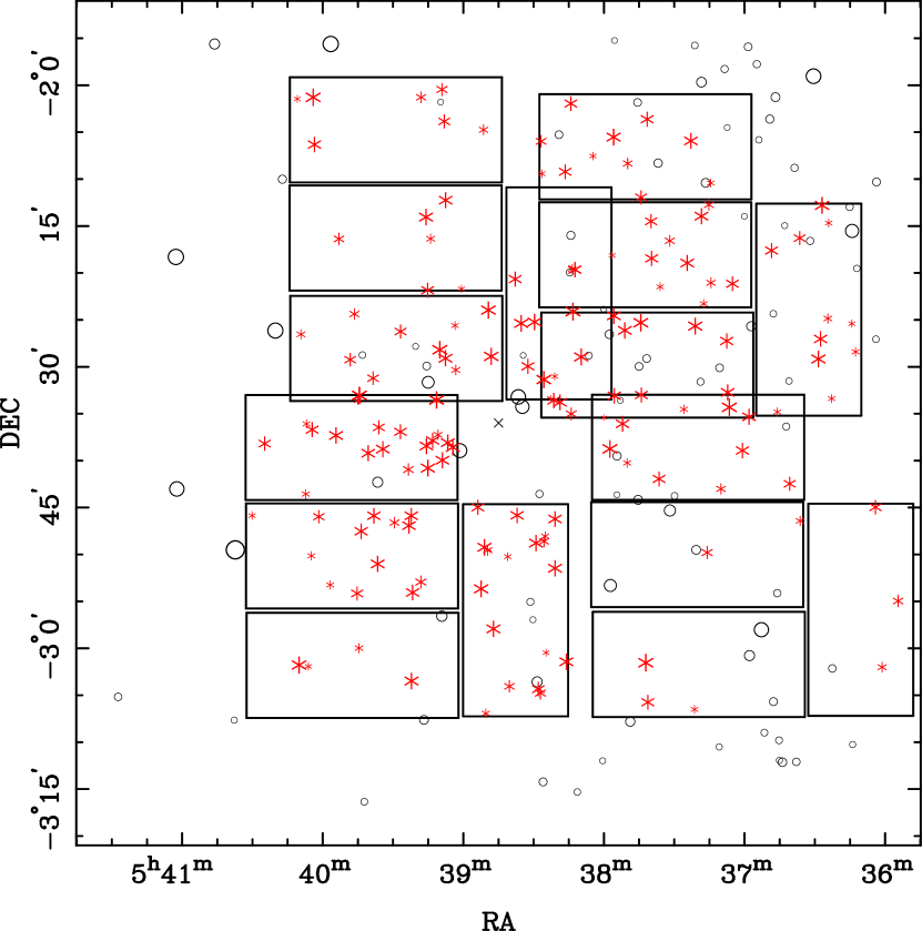
Figure 1.— Representation of present survey in the $\sigma$ Orionis cluster Area covered by the four detectors of each pointing are shown in squares. Field stars brighter than 12 mag are indicated by open circles. The 153 selected optical candidates are denoted by stars and red colors (in the electronic version). The size of the symbols is inversely proportional to the $I$ magnitude. The multiple star $\sigma$ Orionis is labeled with a cross indicating central coordinates.

Figure 2.— $I$ vs. $I-Z$ color–magnitude diagrams for the four pointings. The selected objects are indicated by solid circles, while those previously confirmed members are represented by open circles. The completeness and limiting magnitudes are also shown in dashed and solid lines, respectively. The lower envelope for candidates selection is indicated by a thicker solid line.

Figure 3.— $I$ vs. $I-J$ color–magnitude diagram. Open stars represent objects from previous surveys. Solid circles indicate good cluster member candidates following the infrared photometric sequence of the cluster, while those previously confirmed members are also represented by open circles. Open triangles denote likely non-cluster members. Dashed line indicates the lower envelop of bona fide members. The solid lines represent the 1, 3 and 10 Myr isochrones from the Lyon group. Masses for the 3 Myr iscochrone are also indicated.

Figure 4.— Projected surface density of the substellar population vs. the separation in $\alpha$ and $\delta$ to the center of the cluster. The presence of possible contaminants from the $\zeta$ Orionis cluster and the Orion background population can be seen to the north and west of the $\sigma$ Orionis cluster.

Figure 5.— Projected spatial distribution of the substellar population. The best exponential law fit ($\sigma=\sigma_{0}\,e^{-r/r_{0}}$, where $\sigma_{0}$=0.23 obj/arcmin² and $r_{0}$=9.5 arcmin) is also indicated (see text for details). The dashed line histogram at distances larger than 30 arcmin marks the spatial distribution of likely $\sigma$ Orionis cluster candidate members only (after substracting possible Orion background population contaminants).

Figure 6.— Average nearest neighbor distance between $\sigma$ Orionis candidates (solid histogram) as a function of distance to the center of the cluster. For comparison purposes, we also show the mean values (dotted line) and the first and third quartiles (dashed line) of the same estimator obtained from a Monte Carlo simulation of 10,000 clusters with the same radial distribution and area coverage as our survey, and the expected mean values from a Poissonian distribution (solid line) with the same radial surface density as the cluster.

Figure 7.— Nearest neighbor distances of good cluster member candidates (solid histograms) at separations between 10 and 15 arcmin from the center. For comparison purposes, we also show the histogram of the values of simulated clusters (dashed line) and the expected Poissonian distribution (solid line) with the mean surface density of the cluster at these distances.

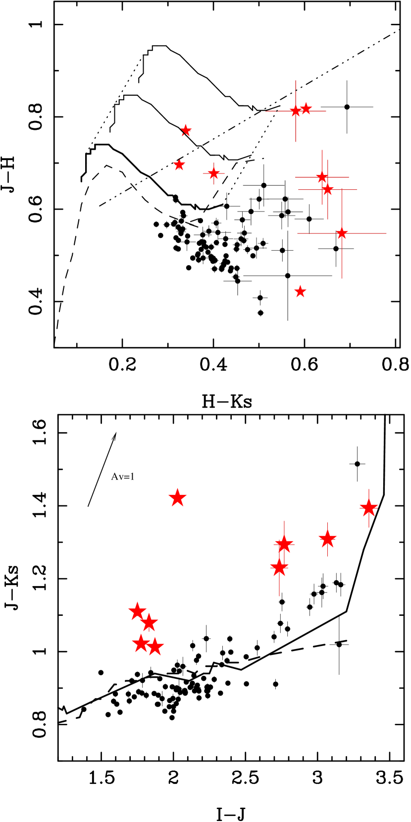
Figure 8.— Upper panel: $J-H$, $H-K_{s}$ color–color diagram of selected candidates (solid circles) with available $JHK_{\rm s}$ photometry from UKIDSS. Objects with near-infrared excesses are indicated by stars and red colors (in the electronic version). The 3 Myr Next Gen isochrone from the Lyon group (Baraffe et al., 1998) reddened with visual extinctions of $A_{V}$ = 0, 1 and 2 are plotted in solid lines from bottom to top (joined by dotted lines). The field dwarf sequence (dashed line) from Bessell & Brett (1988) and Kirkpatrick & McCarthy (1994) and the classical T Tauri star loci (dash-dotted line) from Meyer et al. (1997) are also indicated. Lower panel: $J-K_{s}$, $I-J$ color–color diagram of selected candidates (solid circles) with available $JHK_{\rm s}$ photometry from UKIDSS. Objects with near-infrared excesses are indicated by stars and red colors (in the electronic version). The field M dwarf sequence (solid line) from Bessell & Brett (1988) and Kirkpatrick & McCarthy (1994) and the field M–L dwarf sequence from Leggett et al. (2002) (dashed line) are also indicated.

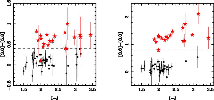
Figure 9.— Left panel: $[3.6]-[5.8]$, $I-J$ color–color diagram of candidates (solid circles) with available photometry from IRAC/Spitzer. Objects with mid-infrared excesses are indicated by stars and red colors (in the electronic version). Right panel: $[3.6]-[8.0]$, $I-J$ color–color diagram of candidates with available photometry from IRAC/Spitzer. Symbols are the same as in the left panel. The horizontal dashed lines indicate our color criteria to identify flux excesses.

Figure 10.— Luminosity function of the selected candidates. A histogram of the number of objects in each bin of magnitude is represented.

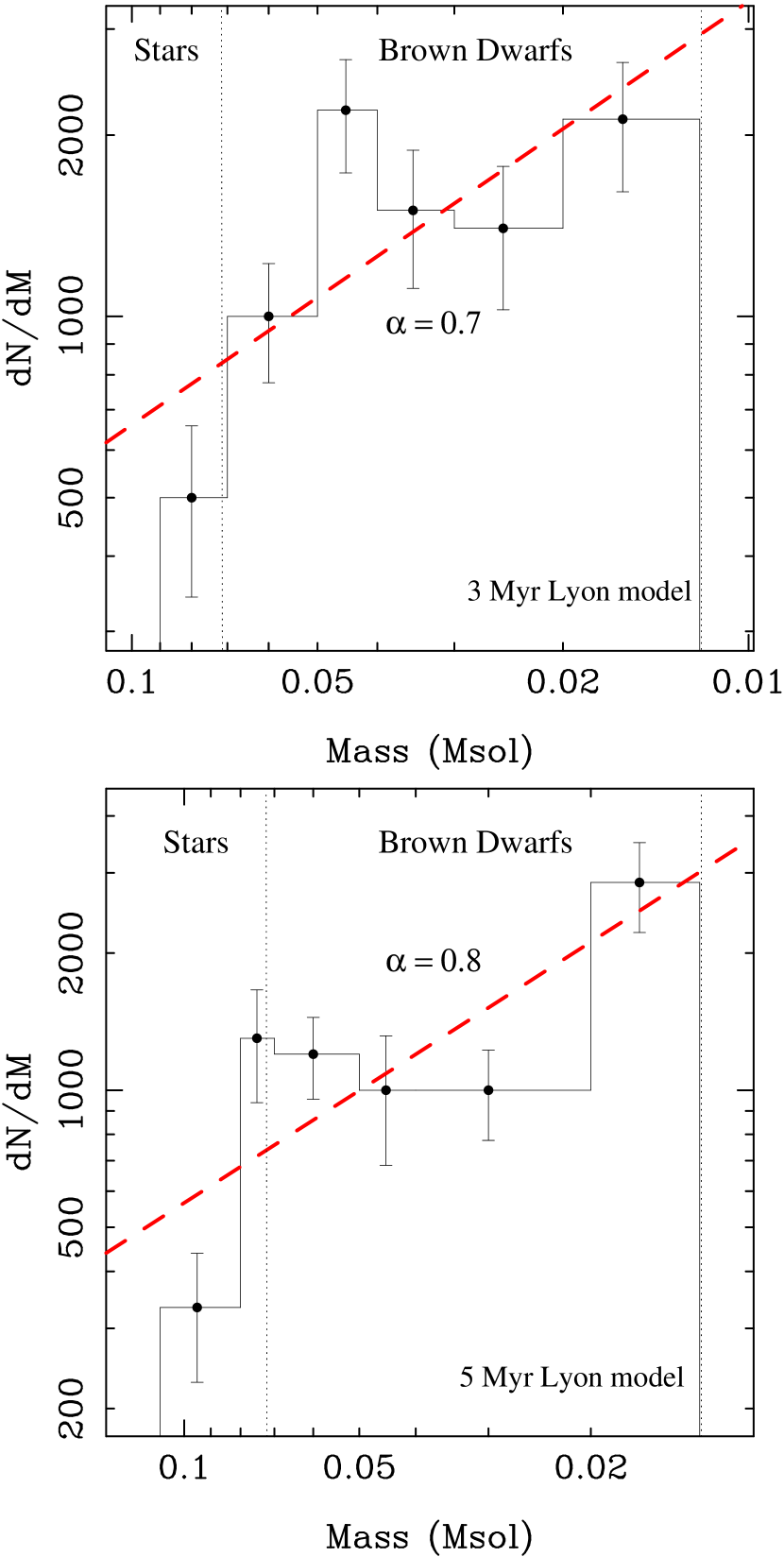
Figure 11.— The mass spectrum of $\sigma$ Orionis. Only bona fide cluster member candidates within the completeness magnitude of present survey have been considered. The theoretical isochrone of 3 Myr (top panel) and 5 Myr (bottom panel) from the Lyon Group (1998) has been used to derive masses. Histograms represent the number of objects per interval of mass ($dN/dm$). The best fit to a potential law ($dN/dm$ $\sim$ m^-α) with an exponent of $\alpha$=0.7 for 3 Myr and 0.8 for 5 Myr is represented by a dashed line (in red in the electronic version).

Table 1 Central coordinates of the four WFC pointings in present survey.

Field	RA (J2000)	DEC (J2000)
	(h m s)	(o ’ ”)
SO1	5 39 06	-02 16 17
SO2	5 37 19	-02 18 04
SO3	5 36 57	-02 50 01
SO4	5 39 25	-02 50 10

Table 2 Photometry and coordinates of survey candiates

Name	prev. ID.	$I$	$I-Z$	$J$	$I-J$	2MASS photometry			R.A.(J2000)	DEC.(J2000)	Membership
						$J$	$H$	$K_{\rm s}$	(h m s)	(o ’ ”)
					SO1 field
					Detector 1
S Ori J053910.02–022811.5	(4)	16.080$\pm$0.040	0.660$\pm$0.040	14.550$\pm$0.050	1.530$\pm$0.060	14.600$\pm$0.030	14.000$\pm$0.040	13.780$\pm$0.050	05 39 10.02	-02 28 11.5	MC
S Ori J053944.33–023302.8	S Ori 11 (1)	16.250$\pm$0.040	0.800$\pm$0.040	14.300$\pm$0.050	1.950$\pm$0.060	14.290$\pm$0.030	13.720$\pm$0.030	13.370$\pm$0.040	05 39 44.33	-02 33 02.8	MC
S Ori J053911.40–023332.7	(3)	16.330$\pm$0.040	0.720$\pm$0.040	14.450$\pm$0.100	1.880$\pm$0.110	14.450$\pm$0.030	13.930$\pm$0.030	13.570$\pm$0.040	05 39 11.40	-02 33 32.7	MC
S Ori J053848.10–022853.7	S Ori 15 (1)	16.380$\pm$0.040	0.810$\pm$0.040	14.480$\pm$0.050	1.910$\pm$0.060	14.470$\pm$0.030	13.840$\pm$0.030	13.440$\pm$0.040	05 38 48.10	-02 28 53.7	MC
S Ori J053849.29–022357.6	(3)	16.410$\pm$0.040	0.670$\pm$0.040	14.230$\pm$0.060	2.180$\pm$0.070	14.360$\pm$0.030	13.700$\pm$0.030	13.200$\pm$0.030	05 38 49.29	-02 23 57.6	MC
S Ori J053907.60–022905.6	S Ori 20 (1)	16.920$\pm$0.040	0.800$\pm$0.040	14.900$\pm$0.050	2.020$\pm$0.060	14.960$\pm$0.040	14.340$\pm$0.040	13.900$\pm$0.050	05 39 07.60	-02 29 05.6	MC
S Ori J053926.77–022614.3	(3)	18.250$\pm$0.040	0.760$\pm$0.040	16.290$\pm$0.050	1.970$\pm$0.060	16.210$\pm$0.090	15.580$\pm$0.100	15.160$\pm$0.170	05 39 26.77	-02 26 14.3	MC
S Ori J053938.50–023113.3	S Ori 41 (1)	18.510$\pm$0.040	0.800$\pm$0.040	16.650$\pm$0.050	1.860$\pm$0.060	16.710$\pm$0.120	15.750$\pm$0.090	15.700$\pm$0.240	05 39 38.50	-02 31 13.3	MC
S Ori J053948.26–022914.3	(3)	18.520$\pm$0.040	0.830$\pm$0.040	16.400$\pm$0.050	2.120$\pm$0.060	16.420$\pm$0.090	15.590$\pm$0.100	15.190$\pm$0.140	05 39 48.26	-02 29 14.3	MC
S Ori J053946.46–022423.2	(3)	19.740$\pm$0.040	1.050$\pm$0.040	17.040$\pm$0.050	2.700$\pm$0.060	17.060$\pm$0.160	16.100$\pm$0.140	15.350$\pm$0.100	05 39 46.46	-02 24 23.2	MC
S Ori J053903.21–023019.9	S Ori 51 (2)	20.320$\pm$0.040	1.150$\pm$0.040	17.210$\pm$0.050	3.110$\pm$0.060	$\cdots$	$\cdots$	$\cdots$	05 39 03.21	-02 30 19.9	MC
S Ori J054009.32–022632.6	(10)	20.550$\pm$0.040	1.140$\pm$0.050	17.720$\pm$0.150	2.830$\pm$0.160	$\cdots$	$\cdots$	$\cdots$	05 40 09.32	-02 26 32.6	MC
S Ori J053903.60–022536.6	S Ori 58 (2)	21.500$\pm$0.050	1.290$\pm$0.060	18.600$\pm$0.050	2.900$\pm$0.070	$\cdots$	$\cdots$	$\cdots$	05 39 03.60	-02 25 36.6	MC
S Ori J053945.12–023335.5		21.570$\pm$0.050	1.090$\pm$0.070	$>$19.0	$<$2.6	$\cdots$	$\cdots$	$\cdots$	05 39 45.12	-02 33 35.5	NM
					Detector 2
S Ori J053813.21–022407.5	S Ori 13 (1)	16.050$\pm$0.030	0.770$\pm$0.040	14.140$\pm$0.050	1.910$\pm$0.060	14.240$\pm$0.030	13.580$\pm$0.030	13.250$\pm$0.040	05 38 13.21	-02 24 07.5	MC
S Ori J053825.68–023121.7	S Ori 18 (1)	16.530$\pm$0.030	0.670$\pm$0.030	14.610$\pm$0.050	1.930$\pm$0.060	14.670$\pm$0.060	14.070$\pm$0.060	13.840$\pm$0.060	05 38 25.68	-02 31 21.7	MC
S Ori J053835.35–022522.2	S Ori 22 (1)	16.750$\pm$0.030	0.760$\pm$0.030	14.640$\pm$0.050	2.110$\pm$0.060	14.650$\pm$0.030	14.060$\pm$0.040	13.760$\pm$0.040	05 38 35.35	-02 25 22.2	MC
S Ori J053829.62–022514.2	S Ori 29 (1)	16.870$\pm$0.030	0.720$\pm$0.030	15.130$\pm$0.050	1.740$\pm$0.060	14.840$\pm$0.030	14.290$\pm$0.030	13.960$\pm$0.060	05 38 29.62	-02 25 14.2	MC
S Ori J053832.44–022957.3	S Ori 39	17.560$\pm$0.030	0.810$\pm$0.030	15.450$\pm$0.060	2.110$\pm$0.070	15.440$\pm$0.060	14.840$\pm$0.060	14.440$\pm$0.090	05 38 32.44	-02 29 57.3	MC
S Ori J053812.40–021938.8	(6)	17.640$\pm$0.030	0.840$\pm$0.030	15.540$\pm$0.090	2.100$\pm$0.090	15.490$\pm$0.060	14.940$\pm$0.060	14.520$\pm$0.090	05 38 12.40	-02 19 38.8	MC
S Ori J053837.88–022039.8	(6)	17.710$\pm$0.030	0.770$\pm$0.030	15.760$\pm$0.030	1.950$\pm$0.040	15.600$\pm$0.060	14.920$\pm$0.040	14.640$\pm$0.090	05 38 37.88	-02 20 39.8	MC
S Ori J053813.56–021934.7		20.770$\pm$0.030	0.970$\pm$0.050	18.560$\pm$0.200	2.210$\pm$0.200	$\cdots$	$\cdots$	$\cdots$	05 38 13.56	-02 19 34.7	NM
					Detector 3
S Ori J054004.13–020117.6		16.220$\pm$0.030	0.680$\pm$0.030	14.190$\pm$0.090	2.030$\pm$0.090	14.300$\pm$0.030	13.640$\pm$0.030	13.410$\pm$0.040	05 40 04.13	-02 01 17.6	OB
S Ori J054003.55–020619.0		17.450$\pm$0.030	0.880$\pm$0.030	15.030$\pm$0.070	2.420$\pm$0.080	14.980$\pm$0.040	14.380$\pm$0.040	13.910$\pm$0.050	05 40 03.55	-02 06 19.0	MC
S Ori J053908.13–020351.4		18.400$\pm$0.030	0.790$\pm$0.030	15.990$\pm$0.120	2.410$\pm$0.120	16.020$\pm$0.070	15.340$\pm$0.070	15.180$\pm$0.160	05 39 08.13	-02 03 51.4	OB
S Ori J053909.10–020026.8		18.840$\pm$0.030	0.900$\pm$0.030	16.270$\pm$0.110	2.570$\pm$0.110	16.170$\pm$0.080	15.560$\pm$0.080	15.410$\pm$0.200	05 39 09.10	-02 00 26.8	OB
S Ori J053918.02–020117.5		19.700$\pm$0.030	0.920$\pm$0.030	17.100$\pm$0.150	2.600$\pm$0.150	16.890$\pm$0.130	16.240$\pm$0.180	15.260$\pm$0.100	05 39 18.02	-02 01 17.5	OB
S Ori J053851.38–020444.6		20.240$\pm$0.030	0.990$\pm$0.030	17.100$\pm$0.150	3.140$\pm$0.150	$\cdots$	$\cdots$	$\cdots$	05 38 51.38	-02 04 44.6	OB
S Ori J054010.85–020127.9		21.920$\pm$0.080	1.180$\pm$0.120	18.810$\pm$0.220	3.110$\pm$0.230	$\cdots$	$\cdots$	$\cdots$	05 40 10.85	-02 01 27.9	OB
					Detector 4
S Ori J053915.96–021403.0	(10)	16.760$\pm$0.040	0.780$\pm$0.040	14.670$\pm$0.150	2.090$\pm$0.160	14.710$\pm$0.040	14.030$\pm$0.040	13.780$\pm$0.060	05 39 15.96	-02 14 03.0	MC
S Ori J053907.56–021214.6	(10)	17.160$\pm$0.030	0.760$\pm$0.030	15.020$\pm$0.040	2.140$\pm$0.050	15.010$\pm$0.030	14.300$\pm$0.040	13.820$\pm$0.050	05 39 07.56	-02 12 14.6	MC
S Ori J053915.26–022150.7	S Ori 38 (1)	17.700$\pm$0.030	0.780$\pm$0.030	15.510$\pm$0.050	2.190$\pm$0.060	15.610$\pm$0.050	14.930$\pm$0.050	14.560$\pm$0.080	05 39 15.26	-02 21 50.7	MC
S Ori J053953.06–021622.9		19.320$\pm$0.030	0.870$\pm$0.030	16.710$\pm$0.080	2.610$\pm$0.090	16.830$\pm$0.130	16.080$\pm$0.130	15.350$\pm$0.190	05 39 53.06	-02 16 22.9	MC
S Ori J053913.95–021621.8	(10)	20.540$\pm$0.030	0.980$\pm$0.030	17.570$\pm$0.100	2.970$\pm$0.100	$\cdots$	$\cdots$	$\cdots$	05 39 13.95	-02 16 21.8	MC
S Ori J053900.79–022141.8	S Ori 56 (2)	21.800$\pm$0.050	1.090$\pm$0.060	18.170$\pm$0.150	3.630$\pm$0.160	$\cdots$	$\cdots$	$\cdots$	05 39 00.79	-02 21 41.8	MC
					SO2 field
					Detector 1
S Ori J053706.49–023419.4		16.130$\pm$0.040	0.690$\pm$0.040	14.750$\pm$0.005	1.380$\pm$0.040	14.700$\pm$0.040	14.170$\pm$0.050	13.920$\pm$0.060	05 37 06.49	-02 34 19.4	MC
S Ori J053744.24–022518.5		16.270$\pm$0.040	0.670$\pm$0.040	14.769$\pm$0.005	1.500$\pm$0.040	14.760$\pm$0.030	14.170$\pm$0.040	13.820$\pm$0.040	05 37 44.24	-02 25 18.5	MC
S Ori J053809.66–022857.0		16.540$\pm$0.040	0.650$\pm$0.040	15.160$\pm$0.006	1.380$\pm$0.040	15.190$\pm$0.050	14.460$\pm$0.050	14.150$\pm$0.070	05 38 09.66	-02 28 57.0	NM
S Ori J053825.68–023121.7	S Ori 18 (1)	16.590$\pm$0.040	0.840$\pm$0.040	14.610$\pm$0.050	1.990$\pm$0.060	14.670$\pm$0.060	14.070$\pm$0.060	13.840$\pm$0.060	05 38 25.68	-02 31 21.7	MC
S Ori J053721.06–022540.0	S Ori 19 (1)	16.620$\pm$0.040	0.820$\pm$0.040	14.720$\pm$0.050	1.900$\pm$0.060	14.770$\pm$0.040	14.140$\pm$0.050	13.920$\pm$0.070	05 37 21.06	-02 25 40.0	MC
S Ori J053751.11–022607.5	S Ori 23 (1)	16.880$\pm$0.040	0.890$\pm$0.040	14.840$\pm$0.050	2.040$\pm$0.060	14.920$\pm$0.040	14.370$\pm$0.040	13.950$\pm$0.060	05 37 51.11	-02 26 07.5	MC
S Ori J053755.74–022433.7	S Ori 24 (1)	16.900$\pm$0.040	0.810$\pm$0.040	15.040$\pm$0.050	1.860$\pm$0.060	15.010$\pm$0.040	14.430$\pm$0.040	14.140$\pm$0.060	05 37 55.74	-02 24 33.7	MC
S Ori J053707.21–023244.2	S Ori 34 (1)	17.100$\pm$0.040	0.770$\pm$0.040	15.330$\pm$0.040	1.770$\pm$0.060	15.540$\pm$0.080	15.090$\pm$0.090	14.600$\pm$0.110	05 37 07.21	-02 32 44.2	MC
S Ori J053818.75–023347.1		17.110$\pm$0.040	0.700$\pm$0.040	15.681$\pm$0.008	1.430$\pm$0.040	15.700$\pm$0.050	15.040$\pm$0.060	14.740$\pm$0.090	05 38 18.75	-02 33 47.1	NM
S Ori J053755.59–023305.3	S Ori 35 (1)	17.360$\pm$0.040	0.950$\pm$0.040	15.180$\pm$0.050	2.190$\pm$0.060	15.220$\pm$0.050	14.590$\pm$0.050	14.190$\pm$0.060	05 37 55.59	-02 33 05.3	MC
S Ori J053821.39–023336.2	(3)	17.450$\pm$0.040	0.950$\pm$0.040	15.300$\pm$0.060	2.150$\pm$0.070	15.360$\pm$0.040	14.790$\pm$0.050	14.490$\pm$0.090	05 38 21.39	-02 33 36.2	MC
S Ori J053707.61–022715.0	S Ori 37 (1)	17.490$\pm$0.040	0.950$\pm$0.040	15.318$\pm$0.006	2.170$\pm$0.040	15.430$\pm$0.060	14.880$\pm$0.080	14.560$\pm$0.100	05 37 07.61	-02 27 15.0	MC
S Ori J053744.05–023300.5		17.590$\pm$0.040	0.740$\pm$0.040	16.067$\pm$0.011	1.520$\pm$0.040	16.090$\pm$0.070	15.400$\pm$0.100	15.160$\pm$0.160	05 37 44.05	-02 33 00.5	NM
S Ori J053813.96–023501.3	S Ori 43 (1)	18.990$\pm$0.040	0.880$\pm$0.040	16.790$\pm$0.050	2.200$\pm$0.060	16.850$\pm$0.160	16.090$\pm$0.150	15.800$\pm$0.250	05 38 13.96	-02 35 01.3	MC
S Ori J053820.99–023101.6		21.880$\pm$0.070	1.490$\pm$0.100	20.020$\pm$0.160	1.860$\pm$0.170	$\cdots$	$\cdots$	$\cdots$	05 38 20.99	-02 31 01.6	NM
S Ori J053822.59–023325.9		22.040$\pm$0.090	1.690$\pm$0.100	$\cdots$	$\cdots$	$\cdots$	$\cdots$	$\cdots$	05 38 22.59	-02 33 25.9
S Ori J053759.96–023525.2		22.690$\pm$0.130	2.030$\pm$0.160	$\cdots$	$\cdots$	$\cdots$	$\cdots$	$\cdots$	05 37 59.96	-02 35 25.2
					Detector 2
S Ori J053626.95–021248.3		16.610$\pm$0.030	0.790$\pm$0.030	15.050$\pm$0.010	1.560$\pm$0.030	14.960$\pm$0.040	14.400$\pm$0.060	14.130$\pm$0.050	05 36 26.95	-02 12 48.3	OB
S Ori J053628.47–022910.4		16.670$\pm$0.030	0.750$\pm$0.030	15.040$\pm$0.050	1.630$\pm$0.060	15.130$\pm$0.040	14.470$\pm$0.060	14.210$\pm$0.050	05 36 28.47	-02 29 10.4	OB
S Ori J053627.58–022702.1		17.350$\pm$0.030	0.820$\pm$0.030	15.670$\pm$0.050	1.680$\pm$0.060	15.620$\pm$0.060	15.010$\pm$0.080	14.510$\pm$0.060	05 36 27.58	-02 27 02.1	OB
S Ori J053648.44–021736.8		17.640$\pm$0.030	0.880$\pm$0.030	15.750$\pm$0.060	1.890$\pm$0.070	15.690$\pm$0.060	15.160$\pm$0.080	14.720$\pm$0.080	05 36 48.44	-02 17 36.8	MC
S Ori J053636.45–021617.1		18.330$\pm$0.030	0.870$\pm$0.030	16.390$\pm$0.040	1.940$\pm$0.050	16.520$\pm$0.110	15.980$\pm$0.150	15.750$\pm$0.180	05 36 36.45	-02 16 17.1	OB
S Ori J053624.43–022451.2		20.640$\pm$0.030	1.190$\pm$0.040	17.790$\pm$0.040	2.850$\pm$0.050	$\cdots$	$\cdots$	$\cdots$	05 36 24.43	-02 24 51.2	OB
S Ori J053612.63–022823.9		21.060$\pm$0.040	1.020$\pm$0.050	18.270$\pm$0.060	2.800$\pm$0.070	$\cdots$	$\cdots$	$\cdots$	05 36 12.63	-02 28 23.9	OB
S Ori J053645.96–023449.6		21.370$\pm$0.050	1.120$\pm$0.070	$>$19.0	$<$2.4	$\cdots$	$\cdots$	$\cdots$	05 36 45.96	-02 34 49.6	NM
S Ori J053622.80–023324.2		21.420$\pm$0.050	1.060$\pm$0.080	19.340$\pm$0.170	2.090$\pm$0.180	$\cdots$	$\cdots$	$\cdots$	05 36 22.80	-02 33 24.2	NM
S Ori J053624.10–021441.3		21.570$\pm$0.050	1.370$\pm$0.070	18.410$\pm$0.070	3.160$\pm$0.080	$\cdots$	$\cdots$	$\cdots$	05 36 24.10	-02 14 41.3	OB
S Ori J053614.20–022523.9		21.760$\pm$0.060	1.130$\pm$0.090	$>$19.0	$<$2.8	$\cdots$	$\cdots$	$\cdots$	05 36 14.20	-02 25 23.9
					Detector 3
S Ori J053755.88–020531.7		16.740$\pm$0.030	0.770$\pm$0.030	14.790$\pm$0.070	1.950$\pm$0.080	14.840$\pm$0.040	14.240$\pm$0.040	13.940$\pm$0.050	05 37 55.88	-02 05 31.7	OB
S Ori J053722.88–020555.9		17.190$\pm$0.030	0.740$\pm$0.030	15.570$\pm$0.050	1.620$\pm$0.060	15.520$\pm$0.070	14.980$\pm$0.100	14.620$\pm$0.110	05 37 22.88	-02 05 55.9	OB
S Ori J053741.56–020337.8		17.620$\pm$0.030	0.740$\pm$0.030	15.660$\pm$0.130	1.960$\pm$0.130	15.780$\pm$0.060	15.190$\pm$0.080	14.890$\pm$0.120	05 37 41.56	-02 03 37.8	OB
S Ori J053814.15–020157.1		17.770$\pm$0.030	0.810$\pm$0.030	15.740$\pm$0.100	2.030$\pm$0.100	15.850$\pm$0.060	15.190$\pm$0.070	14.800$\pm$0.100	05 38 14.15	-02 01 57.1	OB
S Ori J053816.57–020913.2	(10)	17.870$\pm$0.030	0.760$\pm$0.030	15.820$\pm$0.040	2.050$\pm$0.050	15.910$\pm$0.060	15.390$\pm$0.080	15.010$\pm$0.130	05 38 16.57	-02 09 13.2	MC
S Ori J053744.13–021157.0		18.270$\pm$0.030	0.770$\pm$0.030	16.460$\pm$0.050	1.810$\pm$0.060	16.510$\pm$0.110	15.690$\pm$0.090	15.240$\pm$0.160	05 37 44.13	-02 11 57.0	MC
S Ori J053826.86–020558.8		19.140$\pm$0.030	0.990$\pm$0.030	16.500$\pm$0.070	2.640$\pm$0.080	16.500$\pm$0.100	16.080$\pm$0.140	15.310$\pm$0.170	05 38 26.86	-02 05 58.8	OB
S Ori J053749.89–020820.8		19.930$\pm$0.040	0.970$\pm$0.060	18.100$\pm$0.200	1.830$\pm$0.200	$\cdots$	$\cdots$	$\cdots$	05 37 49.89	-02 08 20.8	NM
S Ori J053714.40–021024.7		21.370$\pm$0.060	1.300$\pm$0.090	19.310$\pm$0.150	2.060$\pm$0.160	$\cdots$	$\cdots$	$\cdots$	05 37 14.40	-02 10 24.7	NM
S Ori J053826.49–020925.7		21.530$\pm$0.060	1.240$\pm$0.080	18.250$\pm$0.070	3.280$\pm$0.090	$\cdots$	$\cdots$	$\cdots$	05 38 26.49	-02 09 25.7	MC
S Ori J053804.72–020733.0		21.740$\pm$0.050	1.390$\pm$0.080	18.840$\pm$0.240	2.900$\pm$0.250	$\cdots$	$\cdots$	$\cdots$	05 38 04.72	-02 07 33.0	MC
					Detector 4
S Ori J053718.41–021357.1		17.070$\pm$0.030	0.760$\pm$0.030	15.140$\pm$0.050	1.930$\pm$0.060	15.320$\pm$0.050	14.850$\pm$0.080	14.570$\pm$0.090	05 37 18.41	-02 13 57.1	MC
S Ori J053724.47–021856.5	M1580310 (9)	17.050$\pm$0.030	0.830$\pm$0.030	15.140$\pm$0.110	1.910$\pm$0.110	15.070$\pm$0.050	14.470$\pm$0.060	14.150$\pm$0.070	05 37 24.47	-02 18 56.5	MC
S Ori J053739.66–021826.9	(6)	17.550$\pm$0.030	0.920$\pm$0.030	15.460$\pm$0.140	2.090$\pm$0.140	15.440$\pm$0.050	14.840$\pm$0.050	14.400$\pm$0.070	05 37 39.66	-02 18 26.9	MC
S Ori J053812.40–021938.8	(6)	17.620$\pm$0.030	0.920$\pm$0.030	15.540$\pm$0.010	2.080$\pm$0.030	15.490$\pm$0.060	14.940$\pm$0.060	14.520$\pm$0.090	05 38 12.40	-02 19 38.8	MC
S Ori J053705.17–022109.4	M1738301 (9)	17.790$\pm$0.030	0.980$\pm$0.030	15.660$\pm$0.050	2.130$\pm$0.060	15.420$\pm$0.070	14.780$\pm$0.070	14.310$\pm$0.090	05 37 05.17	-02 21 09.4	MC
S Ori J053739.89–021430.2		18.140$\pm$0.030	0.770$\pm$0.030	16.352$\pm$0.012	1.790$\pm$0.030	16.350$\pm$0.090	15.760$\pm$0.120	$>$16.290	05 37 39.89	-02 14 30.2	MC
S Ori J053731.89–021634.6		19.630$\pm$0.030	0.950$\pm$0.030	17.460$\pm$0.090	2.170$\pm$0.090	$\cdots$	$\cdots$	$\cdots$	05 37 31.89	-02 16 34.6	NM
S Ori J053715.22–021244.2		19.720$\pm$0.030	0.910$\pm$0.030	17.230$\pm$0.070	2.490$\pm$0.080	$\cdots$	$\cdots$	$\cdots$	05 37 15.22	-02 12 44.2	MC
S Ori J053714.33–022102.7		20.200$\pm$0.050	1.030$\pm$0.090	18.920$\pm$0.200	1.280$\pm$0.210	$\cdots$	$\cdots$	$\cdots$	05 37 14.33	-02 21 02.7	NM
S Ori J053717.43–022317.2		21.260$\pm$0.080	1.070$\pm$0.090	$>$19.0	$<$2.3	$\cdots$	$\cdots$	$\cdots$	05 37 17.43	-02 23 17.2	NM
S Ori J053735.99–022128.8		21.420$\pm$0.030	1.050$\pm$0.070	19.880$\pm$0.240	1.540$\pm$0.250	$\cdots$	$\cdots$	$\cdots$	05 37 35.99	-02 21 28.8	NM
S Ori J053756.53–021808.2		21.980$\pm$0.080	1.330$\pm$0.120	$>$19.0	$<$3. 0	$\cdots$	$\cdots$	$\cdots$	05 37 56.53	-02 18 08.2	NM
					SO3 field
					Detector 1
S Ori J053742.15–030132.0		16.090$\pm$0.040	0.720$\pm$0.040	14.410$\pm$0.030	1.680$\pm$0.050	14.530$\pm$0.030	13.940$\pm$0.030	13.590$\pm$0.040	05 37 42.15	-03 01 32.0	MC
S Ori J053741.24–030545.5		17.700$\pm$0.040	0.960$\pm$0.040	15.720$\pm$0.090	1.980$\pm$0.100	15.580$\pm$0.060	14.950$\pm$0.060	14.610$\pm$0.110	05 37 41.24	-03 05 45.5	MC
S Ori J053721.34–030631.4		21.390$\pm$0.050	1.260$\pm$0.060	18.120$\pm$0.110	3.270$\pm$0.120	$\cdots$	$\cdots$	$\cdots$	05 37 21.34	-03 06 31.4	MC
					Detector 2
S Ori J053604.09–024458.1		18.040$\pm$0.030	0.780$\pm$0.030	16.290$\pm$0.090	1.750$\pm$0.090	15.970$\pm$0.080	15.430$\pm$0.100	15.150$\pm$0.100	05 36 04.09	-02 44 58.1	OB
S Ori J053554.47–025458.0		19.460$\pm$0.030	0.920$\pm$0.030	17.090$\pm$0.100	2.370$\pm$0.100	$\cdots$	$\cdots$	$\cdots$	05 35 54.47	-02 54 58.0	OB
S Ori J053601.30–030200.9		20.290$\pm$0.030	1.060$\pm$0.030	17.200$\pm$0.100	3.090$\pm$0.100	$\cdots$	$\cdots$	$\cdots$	05 36 01.30	-03 02 00.9	OB
					Detector 3
S Ori J053757.46–023844.5	S Ori 12 (1)	16.160$\pm$0.030	0.810$\pm$0.030	14.210$\pm$0.050	1.950$\pm$0.060	14.230$\pm$0.030	13.630$\pm$0.030	13.290$\pm$0.030	05 37 57.46	-02 38 44.5	MC
S Ori J053658.07–023519.4	S Ori 33 (1)	17.080$\pm$0.030	0.810$\pm$0.030	15.100$\pm$0.050	1.980$\pm$0.060	15.150$\pm$0.040	14.510$\pm$0.040	14.170$\pm$0.050	05 36 58.07	-02 35 19.4	MC
S Ori J053752.07–023604.6	(6)	17.190$\pm$0.030	0.810$\pm$0.030	15.320$\pm$0.060	1.870$\pm$0.070	15.140$\pm$0.040	14.550$\pm$0.040	14.200$\pm$0.060	05 37 52.07	-02 36 04.6	MC
S Ori J053700.89–023855.6	(5)	17.430$\pm$0.030	0.780$\pm$0.030	15.510$\pm$0.150	1.920$\pm$0.150	15.460$\pm$0.070	14.920$\pm$0.080	14.630$\pm$0.120	05 37 00.89	-02 38 55.6	MC
S Ori J053736.48–024156.7	S Ori 40 (1)	17.790$\pm$0.030	0.900$\pm$0.030	15.490$\pm$0.060	2.290$\pm$0.070	15.470$\pm$0.050	14.940$\pm$0.050	14.560$\pm$0.100	05 37 36.48	-02 41 56.7	MC
S Ori J053640.71–024228.2		18.300$\pm$0.030	0.840$\pm$0.030	16.360$\pm$0.040	1.940$\pm$0.050	16.160$\pm$0.080	15.300$\pm$0.090	15.260$\pm$0.110	05 36 40.71	-02 42 28.2	MC
S Ori J053710.06–024301.4	(5)	19.960$\pm$0.030	1.080$\pm$0.030	16.800$\pm$0.300	3.200$\pm$0.300	$\cdots$	$\cdots$	$\cdots$	05 37 10.06	-02 43 01.4	MC
S Ori J053750.12–024015.3		21.000$\pm$0.040	1.020$\pm$0.040	18.590$\pm$0.040	2.410$\pm$0.060	$\cdots$	$\cdots$	$\cdots$	05 37 50.12	-02 40 15.3	NM
S Ori J053725.88–023432.1	S Ori 55 (2)	21.070$\pm$0.040	1.070$\pm$0.050	18.300$\pm$0.070	2.770$\pm$0.080	$\cdots$	$\cdots$	$\cdots$	05 37 25.88	-02 34 32.1	MC
					Detector 4
S Ori J053715.97–024947.4	(10)	18.890$\pm$0.030	0.970$\pm$0.030	16.350$\pm$0.080	2.540$\pm$0.090	$\cdots$	$\cdots$	$\cdots$	05 37 15.97	-02 49 47.4	MC
S Ori J053636.31–024625.2		20.670$\pm$0.030	1.220$\pm$0.040	17.200$\pm$0.110	3.470$\pm$0.110	$\cdots$	$\cdots$	$\cdots$	05 36 36.31	-02 46 25.2	OB
					SO4 field
					Detector 1
S Ori J054010.09–030147.4		16.400$\pm$0.040	0.650$\pm$0.040	14.774$\pm$0.005	1.630$\pm$0.040	14.840$\pm$0.030	14.260$\pm$0.040	13.960$\pm$0.060	05 40 10.09	-03 01 47.4	MC
S Ori J053922.14–030329.3		16.800$\pm$0.040	0.690$\pm$0.040	15.094$\pm$0.006	1.710$\pm$0.040	15.150$\pm$0.030	14.530$\pm$0.050	14.120$\pm$0.060	05 39 22.14	-03 03 29.3	MC
S Ori J053944.53–025959.0	(8)	20.750$\pm$0.040	1.090$\pm$0.050	18.410$\pm$0.100	2.340$\pm$0.110	$\cdots$	$\cdots$	$\cdots$	05 39 44.53	-02 59 59.0	NM
S Ori J054006.11–030155.7		21.700$\pm$0.070	1.920$\pm$0.090	$>$19.000	$<$2.700	$\cdots$	$\cdots$	$\cdots$	05 40 06.11	-03 01 55.7	NM
					Detector 2
S Ori J053852.40–025339.6		16.640$\pm$0.030	0.680$\pm$0.030	15.059$\pm$0.006	1.590$\pm$0.030	15.060$\pm$0.040	14.470$\pm$0.040	14.260$\pm$0.070	05 38 52.40	-02 53 39.6	MC
S Ori J053851.00–024913.9	(6)	16.790$\pm$0.030	0.750$\pm$0.030	15.044$\pm$0.005	1.750$\pm$0.030	15.040$\pm$0.040	14.420$\pm$0.030	14.160$\pm$0.070	05 38 51.00	-02 49 13.9	MC
S Ori J053828.96–024847.3	(3)	16.860$\pm$0.030	0.860$\pm$0.030	14.830$\pm$0.030	2.030$\pm$0.040	14.820$\pm$0.040	14.280$\pm$0.040	13.880$\pm$0.060	05 38 28.96	-02 48 47.3	MC
S Ori J053820.90–025128.1	M994201 (9)	16.890$\pm$0.030	0.920$\pm$0.030	14.890$\pm$0.040	2.000$\pm$0.050	14.780$\pm$0.030	14.210$\pm$0.030	13.870$\pm$0.050	05 38 20.90	-02 51 28.1	MC
S Ori J053847.15–025755.7	(8)	16.910$\pm$0.030	0.990$\pm$0.030	14.570$\pm$0.030	2.340$\pm$0.040	14.520$\pm$0.030	13.940$\pm$0.040	13.460$\pm$0.040	05 38 47.15	-02 57 55.7	MC
S Ori J053816.04–030126.5		16.950$\pm$0.030	0.730$\pm$0.030	15.259$\pm$0.006	1.690$\pm$0.030	15.280$\pm$0.040	14.670$\pm$0.050	14.380$\pm$0.080	05 38 16.04	-03 01 26.5	MC
S Ori J053820.88–024613.2	S Ori 31 (1)	17.250$\pm$0.030	0.950$\pm$0.030	15.140$\pm$0.050	2.110$\pm$0.060	15.190$\pm$0.040	14.570$\pm$0.050	14.160$\pm$0.080	05 38 20.88	-02 46 13.2	MC
S Ori J053837.04–024550.1		17.380$\pm$0.030	0.710$\pm$0.030	15.631$\pm$0.008	1.750$\pm$0.030	$\cdots$	$\cdots$	$\cdots$	05 38 37.04	-02 45 50.1	MC
S Ori J053853.82–024458.9	(5)	17.680$\pm$0.030	0.860$\pm$0.030	15.470$\pm$0.050	2.210$\pm$0.060	15.450$\pm$0.040	14.940$\pm$0.050	14.590$\pm$0.090	05 38 53.82	-02 44 58.9	MC
S Ori J053827.96–030421.6	M1720188 (9)	17.950$\pm$0.030	1.040$\pm$0.030	15.670$\pm$0.040	2.280$\pm$0.050	15.600$\pm$0.050	15.070$\pm$0.060	14.660$\pm$0.100	05 38 27.96	-03 04 21.6	MC
S Ori J053827.13–030446.4		18.920$\pm$0.060	0.910$\pm$0.060	16.883$\pm$0.019	2.040$\pm$0.060	$\cdots$	$\cdots$	$\cdots$	05 38 27.13	-03 04 46.4	MC
S Ori J053840.38–030403.2		19.440$\pm$0.030	0.970$\pm$0.030	17.420$\pm$0.060	2.020$\pm$0.070	$\cdots$	$\cdots$	$\cdots$	05 38 40.38	-03 04 03.2	NM
S Ori J053825.59–024836.3	S Ori 45 (1)	19.540$\pm$0.030	1.140$\pm$0.030	16.770$\pm$0.050	2.770$\pm$0.060	16.670$\pm$0.110	16.020$\pm$0.130	15.590$\pm$0.210	05 38 25.59	-02 48 36.3	MC
S Ori J053849.58–024933.3	(8)	20.190$\pm$0.030	1.080$\pm$0.030	17.610$\pm$0.050	2.580$\pm$0.060	$\cdots$	$\cdots$	$\cdots$	05 38 49.58	-02 49 33.3	MC
S Ori J053850.40–030656.0		20.960$\pm$0.040	1.070$\pm$0.050	18.220$\pm$0.060	2.730$\pm$0.070	$\cdots$	$\cdots$	$\cdots$	05 38 50.40	-03 06 56.0	MC
S Ori J053825.12–024802.8	S Ori 53 (2)	20.990$\pm$0.040	1.190$\pm$0.050	17.890$\pm$0.060	3.100$\pm$0.070	$\cdots$	$\cdots$	$\cdots$	05 38 25.12	-02 48 02.8	MC
S Ori J053841.03–025014.0		21.430$\pm$0.040	1.170$\pm$0.060	19.000$\pm$0.300	2.400$\pm$0.300	$\cdots$	$\cdots$	$\cdots$	05 38 41.03	-02 50 14.0	NM
S Ori J053824.71–030028.3		21.940$\pm$0.030	1.430$\pm$0.070	18.820$\pm$0.100	3.110$\pm$0.100	$\cdots$	$\cdots$	$\cdots$	05 38 24.71	-03 00 28.3	MC
					Detector 3
S Ori J053911.40–023332.7	(6)	16.330$\pm$0.030	0.750$\pm$0.030	14.460$\pm$0.030	1.870$\pm$0.040	14.450$\pm$0.030	13.930$\pm$0.030	13.570$\pm$0.040	05 39 11.40	-02 33 32.7	MC
S Ori J053944.33–023302.8	S Ori 11 (1)	16.280$\pm$0.030	0.780$\pm$0.030	14.300$\pm$0.050	1.980$\pm$0.060	14.290$\pm$0.030	13.720$\pm$0.030	13.370$\pm$0.040	05 39 44.33	-02 33 02.8	MC
S Ori J053915.10–024047.6	S Ori 16 (1)	16.700$\pm$0.030	0.860$\pm$0.030	14.810$\pm$0.050	1.890$\pm$0.060	14.670$\pm$0.030	14.040$\pm$0.030	13.660$\pm$0.050	05 39 15.10	-02 40 47.6	MC
S Ori J053904.49–023835.4	S Ori 17 (1)	16.800$\pm$0.030	0.810$\pm$0.030	14.770$\pm$0.050	2.030$\pm$0.060	14.770$\pm$0.040	14.190$\pm$0.030	13.800$\pm$0.040	05 39 04.49	-02 38 35.4	MC
S Ori J053954.32–023718.9	(5)	16.920$\pm$0.030	0.850$\pm$0.030	14.670$\pm$0.050	2.250$\pm$0.060	14.750$\pm$0.030	14.210$\pm$0.040	13.800$\pm$0.050	05 39 54.32	-02 37 18.9	MC
S Ori J053906.64–023805.0		16.950$\pm$0.030	0.690$\pm$0.030	15.253$\pm$0.006	1.690$\pm$0.030	$\cdots$	$\cdots$	$\cdots$	05 39 06.64	-02 38 05.0	MC
S Ori J053934.33–023846.8	S Ori 21 (1)	17.010$\pm$0.030	0.920$\pm$0.030	14.760$\pm$0.050	2.260$\pm$0.060	14.760$\pm$0.030	14.190$\pm$0.040	13.790$\pm$0.050	05 39 34.33	-02 38 46.8	MC
S Ori J053908.94–023958.0	S Ori 25 (1)	17.020$\pm$0.030	0.910$\pm$0.030	14.700$\pm$0.050	2.320$\pm$0.060	14.660$\pm$0.030	14.140$\pm$0.040	13.740$\pm$0.050	05 39 08.94	-02 39 58.0	MC
S Ori J053915.76–023826.3	S Ori 26 (1)	17.120$\pm$0.030	0.890$\pm$0.030	14.960$\pm$0.050	2.160$\pm$0.060	$\cdots$	$\cdots$	$\cdots$	05 39 15.76	-02 38 26.3	MC
S Ori J053940.58–023912.4	(7)	17.180$\pm$0.030	0.710$\pm$0.030	15.409$\pm$0.007	1.780$\pm$0.030	15.400$\pm$0.050	14.670$\pm$0.050	14.410$\pm$0.080	05 39 40.58	-02 39 12.4	MC
S Ori J053913.08–023750.9	S Ori 30 (1)	17.300$\pm$0.030	0.820$\pm$0.030	15.250$\pm$0.050	2.040$\pm$0.060	15.240$\pm$0.040	14.750$\pm$0.050	14.310$\pm$0.070	05 39 13.08	-02 37 50.9	MC
S Ori J054004.53–023642.0	(5)	17.680$\pm$0.030	0.900$\pm$0.030	15.400$\pm$0.060	2.280$\pm$0.070	15.310$\pm$0.050	14.810$\pm$0.050	14.270$\pm$0.070	05 40 04.53	-02 36 42.0	MC
S Ori J053926.86–023656.2	S Ori 36 (1)	17.770$\pm$0.030	0.910$\pm$0.030	15.690$\pm$0.050	2.080$\pm$0.060	15.460$\pm$0.040	14.840$\pm$0.050	14.490$\pm$0.070	05 39 26.86	-02 36 56.2	MC
S Ori J054024.79–023810.8	(7)	18.160$\pm$0.030	0.880$\pm$0.030	15.710$\pm$0.020	2.450$\pm$0.040	$\cdots$	$\cdots$	$\cdots$	05 40 24.79	-02 38 10.8	MC
S Ori J053936.08–023627.3	(3)	18.320$\pm$0.030	0.780$\pm$0.040	16.614$\pm$0.016	1.700$\pm$0.040	$\cdots$	$\cdots$	$\cdots$	05 39 36.08	-02 36 27.3	NM
S Ori J053923.43–024057.5	S Ori 42 (1)	19.180$\pm$0.030	1.000$\pm$0.030	16.700$\pm$0.200	2.480$\pm$0.200	16.730$\pm$0.130	15.920$\pm$0.120	15.550$\pm$0.210	05 39 23.43	-02 40 57.5	MC
S Ori J053910.80–023714.6	S Ori 50 (2)	20.520$\pm$0.030	1.040$\pm$0.040	17.530$\pm$0.050	2.980$\pm$0.060	$\cdots$	$\cdots$	$\cdots$	05 39 10.80	-02 37 14.6	MC
S Ori J054007.23–024333.6		21.020$\pm$0.040	1.000$\pm$0.050	18.700$\pm$0.090	2.320$\pm$0.100	$\cdots$	$\cdots$	$\cdots$	05 40 07.23	-02 43 33.6	NM
S Ori J054006.96–023605.0	(8)	21.440$\pm$0.040	1.170$\pm$0.060	18.110$\pm$0.100	3.330$\pm$0.110	$\cdots$	$\cdots$	$\cdots$	05 40 06.96	-02 36 05.0	MC
S Ori J053945.02–023334.1		21.710$\pm$0.050	1.070$\pm$0.080	$>$19.0	$<$2.7	$\cdots$	$\cdots$	$\cdots$	05 39 45.02	-02 33 34.1	NM
					Detector 4
S Ori J053936.58–025100.2		16.980$\pm$0.030	0.680$\pm$0.030	15.200$\pm$0.006	1.790$\pm$0.030	15.240$\pm$0.040	14.680$\pm$0.060	14.360$\pm$0.080	05 39 36.58	-02 51 00.2	MC
S Ori J053922.25–024552.4	(7)	17.150$\pm$0.030	0.710$\pm$0.030	15.341$\pm$0.006	1.810$\pm$0.030	15.320$\pm$0.040	14.830$\pm$0.050	14.410$\pm$0.080	05 39 22.25	-02 45 52.4	MC
S Ori J053923.19–024655.7	S Ori 28 (1)	17.230$\pm$0.030	0.800$\pm$0.030	15.220$\pm$0.050	2.010$\pm$0.060	15.330$\pm$0.040	14.780$\pm$0.040	14.340$\pm$0.070	05 39 23.19	-02 46 55.7	MC
S Ori J053921.66–025403.4		17.290$\pm$0.030	0.710$\pm$0.080	16.461$\pm$0.014	0.830$\pm$0.040	16.290$\pm$0.080	16.040$\pm$0.120	$>$15.760	05 39 21.66	-02 54 03.4	NM
S Ori J053938.16–024552.4	(10)	17.360$\pm$0.030	0.770$\pm$0.030	15.560$\pm$0.050	1.800$\pm$0.060	15.630$\pm$0.060	14.900$\pm$0.060	14.600$\pm$0.090	05 39 38.16	-02 45 52.4	MC
S Ori J053943.59–024731.8	S Ori 32 (1)	17.400$\pm$0.030	0.840$\pm$0.030	15.490$\pm$0.050	1.910$\pm$0.060	15.340$\pm$0.050	14.780$\pm$0.060	14.370$\pm$0.080	05 39 43.59	-02 47 31.8	MC
S Ori J053945.35–025409.0		18.230$\pm$0.030	1.170$\pm$0.090	16.570$\pm$0.080	1.660$\pm$0.090	16.750$\pm$0.110	16.000$\pm$0.120	15.510$\pm$0.200	05 39 45.35	-02 54 09.0	NM
S Ori J054001.65–024558.3		18.710$\pm$0.030	0.910$\pm$0.030	16.760$\pm$0.040	1.950$\pm$0.050	16.770$\pm$0.140	16.440$\pm$0.180	15.540$\pm$0.200	05 40 01.65	-02 45 58.3	MC
S Ori J053918.13–025256.5	(10)	18.890$\pm$0.030	0.960$\pm$0.030	16.230$\pm$0.030	2.660$\pm$0.040	16.150$\pm$0.080	15.550$\pm$0.100	15.140$\pm$0.130	05 39 18.13	-02 52 56.5	MC
S Ori J053929.37–024636.7	(8)	19.810$\pm$0.030	0.920$\pm$0.030	17.160$\pm$0.050	2.660$\pm$0.060	$\cdots$	$\cdots$	$\cdots$	05 39 29.37	-02 46 36.7	MC
S Ori J054004.85–025008.9		21.300$\pm$0.050	1.020$\pm$0.080	$>$18.000	$<$3.300	$\cdots$	$\cdots$	$\cdots$	05 40 04.85	-02 50 08.9	NM
S Ori J053956.83–025314.6		21.350$\pm$0.040	1.120$\pm$0.050	18.200$\pm$0.060	3.150$\pm$0.070	$\cdots$	$\cdots$	$\cdots$	05 39 56.83	-02 53 14.6	MC
S Ori J054030.14–024551.5		21.610$\pm$0.050	1.040$\pm$0.080	19.720$\pm$0.230	1.890$\pm$0.240	$\cdots$	$\cdots$	$\cdots$	05 40 30.14	-02 45 51.5	NM

References. — (1) Béjar et al. 1999 (BZOR) (2) Zapatero Osorio et al. 2000 (3) Béjar et al. 2001 (BMZO) (4) Zapatero Osorio et al. 2002b (5) Béjar et al. 2004a (6) Kenyon et al. 2005 (7) Burningham et al. 2005 (8) Caballero et al. 2004, 2007 (9) Caballero 2008a (10) Lodieu et al. 2009

Table 3 UKIDSS and IRAC photometry

		UKIDSS						IRAC/Spitzer
ID	$I$	$Z$	$Y$	$J$	$H$	$K$		[3.6]	[4.5]	[5.4]	[8.0]	Near/Mid
	(mag)	(mag)	(mag)	(mag)	(mag)	(mag)		(mag)	[(mag)	(mag)	(mag)	IR excess
S Ori J053910.02–022811.5	16.080$\pm$0.040	15.504$\pm$0.005	15.044$\pm$0.004	14.533$\pm$0.004	13.990$\pm$0.004	13.706$\pm$0.004		13.37$\pm$0.04	13.51$\pm$0.04	13.41$\pm$0.06	13.25$\pm$0.11	N/N
S Ori J053944.33–023302.8	16.250$\pm$0.040	15.581$\pm$0.005	14.902$\pm$0.004	14.282$\pm$0.004	13.788$\pm$0.003	13.433$\pm$0.003		13.24$\pm$0.04	13.18$\pm$0.05	12.99$\pm$0.04	12.87$\pm$0.08	N/N
S Ori J053911.40–023332.7	16.330$\pm$0.040	15.687$\pm$0.006	15.057$\pm$0.004	14.437$\pm$0.004	13.904$\pm$0.004	13.581$\pm$0.003		13.30$\pm$0.04	13.20$\pm$0.03	13.10$\pm$0.04	13.02$\pm$0.09	N/N
S Ori J053848.10–022853.7	16.380$\pm$0.040	15.650$\pm$0.006	14.991$\pm$0.004	14.392$\pm$0.004	13.862$\pm$0.004	13.488$\pm$0.003		13.08$\pm$0.05	12.75$\pm$0.06	12.38$\pm$0.03	11.77$\pm$0.05	N/Y
S Ori J053849.29–022357.6	16.410$\pm$0.040	15.851$\pm$0.006	15.241$\pm$0.005	14.536$\pm$0.004	14.115$\pm$0.004	13.524$\pm$0.003		12.76$\pm$0.04	12.52$\pm$0.04	11.94$\pm$0.02	11.58$\pm$0.04	Y/Y
S Ori J053907.60–022905.6	16.920$\pm$0.040	16.201$\pm$0.007	15.553$\pm$0.006	14.874$\pm$0.005	14.299$\pm$0.005	13.928$\pm$0.004		13.54$\pm$0.06	13.60$\pm$0.05	13.43$\pm$0.05	13.57$\pm$0.16	N/N
S Ori J053926.77–022614.3	18.250$\pm$0.040	17.633$\pm$0.017	16.888$\pm$0.014	16.224$\pm$0.012	15.688$\pm$0.016	15.261$\pm$0.015		$\cdots$	14.78$\pm$0.09	14.30$\pm$0.16	13.63$\pm$0.16	N/ $\cdots$
S Ori J053938.50–023113.3	18.510$\pm$0.040	17.870$\pm$0.022	17.285$\pm$0.018	16.590$\pm$0.015	16.061$\pm$0.019	15.719$\pm$0.020		15.26$\pm$0.10	15.22$\pm$0.13	14.70$\pm$0.40	14.20$\pm$0.40	N/Y
S Ori J053948.26–022914.3	18.520$\pm$0.040	17.881$\pm$0.022	17.079$\pm$0.015	16.382$\pm$0.013	15.834$\pm$0.016	15.366$\pm$0.015		15.01$\pm$0.06	14.91$\pm$0.07	14.85$\pm$0.19	$\cdots$	N/N
S Ori J053946.46–022423.2	19.740$\pm$0.040	18.890$\pm$0.050	17.870$\pm$0.030	16.986$\pm$0.022	16.400$\pm$0.030	15.850$\pm$0.030		15.29$\pm$0.08	15.09$\pm$0.08	14.89$\pm$0.21	14.15$\pm$0.22	N/N
S Ori J053903.21–023019.9	20.320$\pm$0.040	19.320$\pm$0.070	18.130$\pm$0.040	17.185$\pm$0.025	16.610$\pm$0.030	16.000$\pm$0.030		15.40$\pm$0.07	15.42$\pm$0.08	15.02$\pm$0.25	14.90$\pm$0.40	N/N
S Ori J054009.32–022632.6	20.550$\pm$0.040	19.480$\pm$0.080	18.300$\pm$0.040	17.390$\pm$0.030	16.880$\pm$0.040	16.210$\pm$0.030		15.52$\pm$0.07	15.57$\pm$0.09	15.20$\pm$0.30	$\cdots$	N/N
S Ori J053903.60–022536.6	21.500$\pm$0.050	20.470$\pm$0.180	19.060$\pm$0.090	18.360$\pm$0.070	17.900$\pm$0.120	17.070$\pm$0.080		16.50$\pm$0.11	16.40$\pm$0.15	15.80$\pm$0.40	$\cdots$	$\cdots$ /Y
S Ori J053945.12-023335.5	21.570$\pm$0.050	$\cdots$	$\cdots$	$\cdots$	$\cdots$	$\cdots$		18.500$\pm$0.500	$\cdots$	$\cdots$	$\cdots$	$\cdots$
S Ori J053813.21–022407.5	16.050$\pm$0.030	15.323$\pm$0.005	14.677$\pm$0.003	14.073$\pm$0.003	13.572$\pm$0.003	13.207$\pm$0.003		12.82$\pm$0.03	12.91$\pm$0.04	12.72$\pm$0.03	12.74$\pm$0.07	N/N
S Ori J053825.68–023121.7	16.530$\pm$0.030	15.868$\pm$0.006	15.211$\pm$0.005	14.592$\pm$0.004	14.078$\pm$0.004	13.756$\pm$0.004		13.42$\pm$0.04	13.49$\pm$0.04	13.43$\pm$0.05	13.22$\pm$0.10	N/N
S Ori J053835.35–022522.2	16.750$\pm$0.030	16.009$\pm$0.007	15.257$\pm$0.005	14.623$\pm$0.004	14.157$\pm$0.004	13.720$\pm$0.004		13.29$\pm$0.04	13.38$\pm$0.08	13.19$\pm$0.05	13.28$\pm$0.11	N/N
S Ori J053829.62–022514.2	16.870$\pm$0.030	16.157$\pm$0.007	15.472$\pm$0.005	14.820$\pm$0.005	14.327$\pm$0.005	13.932$\pm$0.005		13.48$\pm$0.04	13.52$\pm$0.04	13.50$\pm$0.06	13.45$\pm$0.12	N/N
S Ori J053832.44–022957.3	17.560$\pm$0.030	16.863$\pm$0.012	16.078$\pm$0.008	15.382$\pm$0.007	14.889$\pm$0.008	14.490$\pm$0.007		14.03$\pm$0.05	14.08$\pm$0.06	13.89$\pm$0.09	13.82$\pm$0.16	N/N
S Ori J053812.40–021938.8	17.640$\pm$0.030	16.879$\pm$0.011	16.089$\pm$0.008	15.385$\pm$0.007	14.932$\pm$0.008	14.483$\pm$0.008		13.92$\pm$0.06	13.60$\pm$0.05	13.34$\pm$0.05	12.68$\pm$0.10	N/Y
S Ori J053837.88–022039.8	17.710$\pm$0.030	16.893$\pm$0.012	16.159$\pm$0.009	15.471$\pm$0.007	14.990$\pm$0.009	14.567$\pm$0.008		14.17$\pm$0.05	14.17$\pm$0.05	14.26$\pm$0.11	14.40$\pm$0.30	N/N
S Ori J053813.56–021934.7	20.770$\pm$0.030	20.230$\pm$0.170	19.380$\pm$0.120	18.310$\pm$0.070	18.060$\pm$0.130	17.500$\pm$0.120		16.84$\pm$0.14	17.00$\pm$0.30	$\cdots$	$\cdots$	$\cdots$
S Ori J054004.13–020117.6	16.220$\pm$0.030	$\cdots$	$\cdots$	$\cdots$	$\cdots$	$\cdots$		$\cdots$	$\cdots$	$\cdots$	$\cdots$	$\cdots$
S Ori J054003.55–020619.0	17.450$\pm$0.030	16.707$\pm$0.010	15.767$\pm$0.006	14.948$\pm$0.005	14.449$\pm$0.005	13.962$\pm$0.005		$\cdots$	$\cdots$	$\cdots$	$\cdots$	N/ $\cdots$
S Ori J053908.13–020351.4	18.400$\pm$0.030	17.515$\pm$0.017	16.780$\pm$0.013	15.996$\pm$0.011	15.335$\pm$0.011	14.923$\pm$0.012		$\cdots$	$\cdots$	$\cdots$	$\cdots$	Y/ $\cdots$
S Ori J053909.10–020026.8	18.840$\pm$0.030	$\cdots$	$\cdots$	$\cdots$	$\cdots$	$\cdots$		$\cdots$	$\cdots$	$\cdots$	$\cdots$	$\cdots$
S Ori J053918.02–020117.5	19.700$\pm$0.030	$\cdots$	$\cdots$	$\cdots$	$\cdots$	$\cdots$		$\cdots$	$\cdots$	$\cdots$	$\cdots$	$\cdots$
S Ori J053851.38–020444.6	20.240$\pm$0.030	19.170$\pm$0.070	18.140$\pm$0.040	17.280$\pm$0.030	16.630$\pm$0.040	16.110$\pm$0.030		$\cdots$	$\cdots$	$\cdots$	$\cdots$	N/ $\cdots$
S Ori J054010.85–020127.9	21.920$\pm$0.080	$\cdots$	$\cdots$	$\cdots$	$\cdots$	17.450$\pm$0.100		$\cdots$	$\cdots$	$\cdots$	$\cdots$	$\cdots$
S Ori J053915.96–021403.0	16.760$\pm$0.040	15.952$\pm$0.006	15.281$\pm$0.005	14.604$\pm$0.004	14.124$\pm$0.004	13.702$\pm$0.004		13.25$\pm$0.06	$\cdots$	$\cdots$	$\cdots$	N/ $\cdots$
S Ori J053907.56–021214.6	17.160$\pm$0.030	16.691$\pm$0.010	15.860$\pm$0.007	15.133$\pm$0.006	14.316$\pm$0.005	13.713$\pm$0.004		13.03$\pm$0.04	$\cdots$	$\cdots$	$\cdots$	Y/ $\cdots$
S Ori J053915.26–022150.7	17.700$\pm$0.030	17.151$\pm$0.013	16.300$\pm$0.009	15.526$\pm$0.008	15.014$\pm$0.009	14.539$\pm$0.008		13.79$\pm$0.04	13.66$\pm$0.05	13.06$\pm$0.05	12.64$\pm$0.07	N/Y
S Ori J053953.06–021622.9	19.320$\pm$0.030	18.590$\pm$0.040	17.581$\pm$0.022	16.739$\pm$0.017	16.223$\pm$0.022	15.728$\pm$0.021		15.06$\pm$0.08	$\cdots$	$\cdots$	$\cdots$	N/ $\cdots$
S Ori J053913.95–021621.8	20.540$\pm$0.030	19.700$\pm$0.090	18.540$\pm$0.060	17.510$\pm$0.030	16.860$\pm$0.050	16.350$\pm$0.040		15.72$\pm$0.08	15.46$\pm$0.16	15.50$\pm$0.30	$\cdots$	N/N
S Ori J053900.79–022141.8	21.800$\pm$0.050	$\cdots$	19.970$\pm$0.200	18.360$\pm$0.070	17.780$\pm$0.110	16.870$\pm$0.070		16.10$\pm$0.09	15.89$\pm$0.11	15.40$\pm$0.30	14.90$\pm$0.40	$\cdots$ /Y
S Ori J053706.49–023419.4	16.130$\pm$0.040	15.692$\pm$0.006	15.283$\pm$0.005	14.750$\pm$0.005	14.183$\pm$0.004	13.908$\pm$0.005		$\cdots$	$\cdots$	$\cdots$	$\cdots$	N/ $\cdots$
S Ori J053744.24–022518.5	16.270$\pm$0.040	15.731$\pm$0.006	15.337$\pm$0.005	14.769$\pm$0.005	14.143$\pm$0.004	13.826$\pm$0.004		13.690$\pm$0.060	13.670$\pm$0.050	13.840$\pm$0.080	13.570$\pm$0.130	N/N
S Ori J053809.66–022857.0	16.540$\pm$0.040	16.056$\pm$0.007	15.700$\pm$0.006	15.160$\pm$0.006	14.494$\pm$0.006	14.229$\pm$0.006		13.950$\pm$0.050	14.150$\pm$0.070	14.130$\pm$0.100	13.810$\pm$0.160	N/N
S Ori J053825.68–023121.7	16.590$\pm$0.040	15.868$\pm$0.006	15.211$\pm$0.005	14.592$\pm$0.004	14.078$\pm$0.004	13.756$\pm$0.004		13.42$\pm$0.04	13.49$\pm$0.04	13.43$\pm$0.05	13.22$\pm$0.10	N/N
S Ori J053721.06–022540.0	16.620$\pm$0.040	15.953$\pm$0.006	15.370$\pm$0.005	14.724$\pm$0.004	14.156$\pm$0.004	13.843$\pm$0.004		$\cdots$	$\cdots$	$\cdots$	$\cdots$	N/ $\cdots$
S Ori J053751.11–022607.5	16.880$\pm$0.040	16.192$\pm$0.007	15.521$\pm$0.005	14.856$\pm$0.005	14.335$\pm$0.004	13.956$\pm$0.005		13.64$\pm$0.06	13.58$\pm$0.04	13.80$\pm$0.07	13.49$\pm$0.12	N/N
S Ori J053755.74–022433.7	16.900$\pm$0.040	16.287$\pm$0.008	15.674$\pm$0.006	15.029$\pm$0.005	14.488$\pm$0.004	14.144$\pm$0.006		13.72$\pm$0.04	13.92$\pm$0.06	13.68$\pm$0.07	13.61$\pm$0.13	N/N
S Ori J053707.21–023244.2	17.100$\pm$0.040	16.649$\pm$0.010	16.098$\pm$0.008	15.498$\pm$0.008	14.937$\pm$0.006	14.614$\pm$0.008		$\cdots$	$\cdots$	$\cdots$	$\cdots$	N/ $\cdots$
S Ori J053818.75–023347.1	17.110$\pm$0.040	16.588$\pm$0.010	16.189$\pm$0.009	15.681$\pm$0.008	15.082$\pm$0.009	14.805$\pm$0.009		14.590$\pm$0.080	14.650$\pm$0.070	14.540$\pm$0.150	14.280$\pm$0.220	N/N
S Ori J053755.59–023305.3	17.360$\pm$0.040	16.667$\pm$0.010	15.860$\pm$0.007	15.154$\pm$0.006	14.655$\pm$0.005	14.227$\pm$0.006		13.62$\pm$0.04	13.58$\pm$0.04	13.14$\pm$0.05	12.33$\pm$0.06	N/Y
S Ori J053821.39–023336.2	17.450$\pm$0.040	16.772$\pm$0.011	16.013$\pm$0.008	15.317$\pm$0.007	14.799$\pm$0.007	14.404$\pm$0.007		13.96$\pm$0.07	13.94$\pm$0.05	13.80$\pm$0.11	13.90$\pm$0.19	N/N
S Ori J053707.61–022715.0	17.490$\pm$0.040	16.760$\pm$0.011	16.044$\pm$0.007	15.318$\pm$0.006	14.790$\pm$0.006	14.411$\pm$0.006		$\cdots$	$\cdots$	$\cdots$	$\cdots$	N/ $\cdots$
S Ori J053744.05–023300.5	17.590$\pm$0.040	17.115$\pm$0.013	16.660$\pm$0.011	16.067$\pm$0.011	15.439$\pm$0.010	15.139$\pm$0.012		14.800$\pm$0.060	14.890$\pm$0.080	14.930$\pm$0.230	14.700$\pm$0.300	N/N
S Ori J053813.96–023501.3	18.990$\pm$0.040	18.330$\pm$0.040	17.591$\pm$0.024	16.926$\pm$0.021	16.380$\pm$0.030	15.970$\pm$0.030		15.71$\pm$0.11	15.78$\pm$0.12	15.30$\pm$0.30	$\cdots$	N/Y
S Ori J053820.99–023101.6	21.880$\pm$0.070	$\cdots$	$\cdots$	$\cdots$	$\cdots$	17.710$\pm$0.130		15.96$\pm$0.14	15.77$\pm$0.13	15.50$\pm$0.40	15.00$\pm$0.40	$\cdots$ /Y
S Ori J053822.59–023325.9	22.040$\pm$0.090	$\cdots$	$\cdots$	$\cdots$	$\cdots$	$\cdots$		16.72$\pm$0.15	16.45$\pm$0.19	$\cdots$	$\cdots$	$\cdots$
S Ori J053759.96–023525.2	22.690$\pm$0.130	$\cdots$	$\cdots$	$\cdots$	$\cdots$	$\cdots$		16.84$\pm$0.16	16.87$\pm$0.23	$\cdots$	$\cdots$	$\cdots$
S Ori J053626.95–021248.3	16.610$\pm$0.030	16.089$\pm$0.007	15.577$\pm$0.005	14.962$\pm$0.005	14.368$\pm$0.004	14.061$\pm$0.005		$\cdots$	$\cdots$	$\cdots$	$\cdots$	N/ $\cdots$
S Ori J053628.47–022910.4	16.670$\pm$0.030	16.235$\pm$0.007	15.720$\pm$0.006	15.085$\pm$0.006	14.481$\pm$0.005	14.175$\pm$0.006		$\cdots$	$\cdots$	$\cdots$	$\cdots$	N/ $\cdots$
S Ori J053627.58–022702.1	17.350$\pm$0.030	16.821$\pm$0.011	16.236$\pm$0.008	15.561$\pm$0.007	14.984$\pm$0.006	14.632$\pm$0.007		$\cdots$	$\cdots$	$\cdots$	$\cdots$	N/ $\cdots$
S Ori J053648.44–021736.8	17.640$\pm$0.030	16.985$\pm$0.013	16.272$\pm$0.008	15.566$\pm$0.007	15.068$\pm$0.007	14.674$\pm$0.008		$\cdots$	$\cdots$	$\cdots$	$\cdots$	N/ $\cdots$
S Ori J053636.45–021617.1	18.330$\pm$0.030	17.757$\pm$0.022	17.062$\pm$0.014	16.430$\pm$0.013	15.897$\pm$0.013	15.543$\pm$0.017		$\cdots$	$\cdots$	$\cdots$	$\cdots$	N/ $\cdots$
S Ori J053624.43–022451.2	20.640$\pm$0.030	19.990$\pm$0.140	18.850$\pm$0.060	17.790$\pm$0.040	17.050$\pm$0.040	16.370$\pm$0.030		$\cdots$	$\cdots$	$\cdots$	$\cdots$	Y/ $\cdots$
S Ori J053612.63–022823.9	21.060$\pm$0.040	$\cdots$	19.540$\pm$0.120	18.270$\pm$0.060	17.500$\pm$0.050	16.980$\pm$0.060		$\cdots$	$\cdots$	$\cdots$	$\cdots$	N/ $\cdots$
S Ori J053645.96–023449.6	21.370$\pm$0.050	$\cdots$	$\cdots$	$\cdots$	18.670$\pm$0.160	17.770$\pm$0.140		$\cdots$	$\cdots$	$\cdots$	$\cdots$	$\cdots$
S Ori J053622.80–023324.2	21.420$\pm$0.050	$\cdots$	20.130$\pm$0.200	19.340$\pm$0.170	18.560$\pm$0.140	17.460$\pm$0.100		$\cdots$	$\cdots$	$\cdots$	$\cdots$	N/ $\cdots$
S Ori J053624.10–021441.3	21.570$\pm$0.050	20.590$\pm$0.210	19.330$\pm$0.090	18.410$\pm$0.070	17.780$\pm$0.060	17.170$\pm$0.070		$\cdots$	$\cdots$	$\cdots$	$\cdots$	N/ $\cdots$
S Ori J053614.20–022523.9	21.760$\pm$0.060	$\cdots$	$\cdots$	$\cdots$	18.880$\pm$0.200	17.760$\pm$0.150		$\cdots$	$\cdots$	$\cdots$	$\cdots$	$\cdots$
S Ori J053755.88–020531.7	16.740$\pm$0.030	16.033$\pm$0.007	15.423$\pm$0.005	14.779$\pm$0.005	14.256$\pm$0.004	13.885$\pm$0.004		$\cdots$	$\cdots$	$\cdots$	$\cdots$	N/ $\cdots$
S Ori J053722.88–020555.9	17.190$\pm$0.030	16.607$\pm$0.009	16.169$\pm$0.008	15.586$\pm$0.007	$\cdots$	14.667$\pm$0.008		$\cdots$	$\cdots$	$\cdots$	$\cdots$	N/ $\cdots$
S Ori J053741.56–020337.8	17.620$\pm$0.030	16.969$\pm$0.012	16.406$\pm$0.009	15.739$\pm$0.008	15.185$\pm$0.007	14.866$\pm$0.009		$\cdots$	$\cdots$	$\cdots$	$\cdots$	N/ $\cdots$
S Ori J053814.15–020157.1	17.770$\pm$0.030	16.997$\pm$0.012	16.335$\pm$0.010	15.672$\pm$0.009	15.149$\pm$0.011	14.760$\pm$0.010		$\cdots$	$\cdots$	$\cdots$	$\cdots$	N/ $\cdots$
S Ori J053816.57–020913.2	17.870$\pm$0.030	17.179$\pm$0.014	16.573$\pm$0.011	15.875$\pm$0.010	15.381$\pm$0.013	15.003$\pm$0.012		14.51$\pm$0.06	$\cdots$	$\cdots$	$\cdots$	N/ $\cdots$
S Ori J053744.13–021157.0	18.270$\pm$0.030	17.605$\pm$0.018	17.116$\pm$0.015	16.424$\pm$0.013	15.872$\pm$0.012	15.482$\pm$0.016		15.20$\pm$0.06	$\cdots$	$\cdots$	$\cdots$	N/ $\cdots$
S Ori J053826.86–020558.8	19.140$\pm$0.030	18.220$\pm$0.030	17.275$\pm$0.020	16.428$\pm$0.015	15.885$\pm$0.020	15.393$\pm$0.017		$\cdots$	$\cdots$	$\cdots$	$\cdots$	N/ $\cdots$
S Ori J053749.89–020820.8	19.930$\pm$0.040	19.110$\pm$0.060	18.920$\pm$0.060	18.430$\pm$0.070	17.730$\pm$0.060	17.590$\pm$0.110		$\cdots$	$\cdots$	$\cdots$	$\cdots$	$\cdots$
S Ori J053714.40–021024.7	21.370$\pm$0.060	$\cdots$	19.910$\pm$0.150	19.310$\pm$0.150	18.610$\pm$0.140	17.820$\pm$0.140		$\cdots$	$\cdots$	$\cdots$	$\cdots$	$\cdots$
S Ori J053826.49–020925.7	21.530$\pm$0.060	$\cdots$	19.080$\pm$0.090	18.250$\pm$0.070	17.490$\pm$0.080	16.850$\pm$0.060		16.220$\pm$0.100	$\cdots$	$\cdots$	$\cdots$	N/ $\cdots$
S Ori J053804.72–020733.0	21.740$\pm$0.050	$\cdots$	$\cdots$	$\cdots$	$\cdots$	$\cdots$		18.40$\pm$0.50	$\cdots$	$\cdots$	$\cdots$	$\cdots$
S Ori J053718.41–021357.1	17.070$\pm$0.030	16.464$\pm$0.008	15.975$\pm$0.007	15.343$\pm$0.006	14.796$\pm$0.005	14.467$\pm$0.007		$\cdots$	$\cdots$	$\cdots$	$\cdots$	N/ $\cdots$
S Ori J053724.47–021856.5	17.050$\pm$0.030	16.423$\pm$0.008	15.830$\pm$0.006	15.145$\pm$0.006	14.552$\pm$0.005	14.219$\pm$0.006		$\cdots$	$\cdots$	$\cdots$	$\cdots$	N/ $\cdots$
S Ori J053739.66–021826.9	17.550$\pm$0.030	16.895$\pm$0.011	16.118$\pm$0.007	15.406$\pm$0.007	14.878$\pm$0.006	14.472$\pm$0.007		13.99$\pm$0.05	14.09$\pm$0.04	13.92$\pm$0.09	13.89$\pm$0.18	N/N
S Ori J053812.40–021938.8	17.620$\pm$0.030	16.879$\pm$0.011	16.089$\pm$0.008	15.385$\pm$0.007	14.932$\pm$0.008	14.483$\pm$0.008		13.92$\pm$0.06	13.60$\pm$0.05	13.34$\pm$0.05	12.68$\pm$0.10	N/Y
S Ori J053705.17–022109.4	17.790$\pm$0.030	17.081$\pm$0.014	16.275$\pm$0.008	15.551$\pm$0.007	15.175$\pm$0.007	14.672$\pm$0.008		$\cdots$	$\cdots$	$\cdots$	$\cdots$	N/ $\cdots$
S Ori J053739.89–021430.2	18.140$\pm$0.030	17.531$\pm$0.017	17.046$\pm$0.014	16.352$\pm$0.012	15.808$\pm$0.012	15.431$\pm$0.015		15.050$\pm$0.060	15.230$\pm$0.080	14.900$\pm$0.200	15.000$\pm$0.500	N/N
S Ori J053731.89–021634.6	19.630$\pm$0.030	18.930$\pm$0.050	18.050$\pm$0.030	17.320$\pm$0.030	16.800$\pm$0.030	16.410$\pm$0.040		16.07$\pm$0.09	16.12$\pm$0.13	15.60$\pm$0.40	$\cdots$	N/Y
S Ori J053715.22–021244.2	19.720$\pm$0.030	19.070$\pm$0.060	18.250$\pm$0.030	17.490$\pm$0.030	16.880$\pm$0.030	16.450$\pm$0.040		$\cdots$	$\cdots$	$\cdots$	$\cdots$	N/ $\cdots$
S Ori J053714.33–022102.7	20.200$\pm$0.050	19.810$\pm$0.130	19.270$\pm$0.090	19.030$\pm$0.120	18.270$\pm$0.110	18.450$\pm$0.240		$\cdots$	$\cdots$	$\cdots$	$\cdots$	$\cdots$
S Ori J053717.43–022317.2	21.260$\pm$0.080	$\cdots$	$\cdots$	$\cdots$	19.140$\pm$0.230	$\cdots$		$\cdots$	$\cdots$	$\cdots$	$\cdots$	$\cdots$
S Ori J053735.99–022128.8	21.420$\pm$0.030	$\cdots$	20.495$\pm$0.300	19.880$\pm$0.240	18.920$\pm$0.190	$\cdots$		18.200$\pm$0.400	$\cdots$	$\cdots$	$\cdots$	N/ $\cdots$
S Ori J053756.53–021808.2	21.980$\pm$0.080	$\cdots$	$\cdots$	$\cdots$	$\cdots$	$\cdots$		$\cdots$	$\cdots$	$\cdots$	$\cdots$	$\cdots$
S Ori J053742.15–030132.0	16.090$\pm$0.040	15.558$\pm$0.005	15.066$\pm$0.004	14.484$\pm$0.004	13.946$\pm$0.004	13.628$\pm$0.004		$\cdots$	$\cdots$	$\cdots$	12.83$\pm$0.10	N/ $\cdots$
S Ori J053741.24–030545.5	17.700$\pm$0.040	16.999$\pm$0.012	16.222$\pm$0.008	15.522$\pm$0.007	15.052$\pm$0.008	14.649$\pm$0.009		$\cdots$	$\cdots$	$\cdots$	$\cdots$	N/ $\cdots$
S Ori J053721.34–030631.4	21.390$\pm$0.050	$\cdots$	19.150$\pm$0.070	18.120$\pm$0.040	17.300$\pm$0.060	16.600$\pm$0.050		$\cdots$	$\cdots$	$\cdots$	$\cdots$	N/ $\cdots$
S Ori J053604.09–024458.1	18.040$\pm$0.030	17.412$\pm$0.016	16.666$\pm$0.011	15.998$\pm$0.010	15.478$\pm$0.009	15.027$\pm$0.012		$\cdots$	$\cdots$	$\cdots$	$\cdots$	N/ $\cdots$
S Ori J053554.47–025458.0	19.460$\pm$0.030	18.830$\pm$0.050	17.910$\pm$0.030	17.175$\pm$0.024	16.610$\pm$0.030	16.210$\pm$0.040		$\cdots$	$\cdots$	$\cdots$	$\cdots$	N/ $\cdots$
S Ori J053601.30–030200.9	20.290$\pm$0.030	19.650$\pm$0.110	18.430$\pm$0.040	17.232$\pm$0.025	16.640$\pm$0.040	16.160$\pm$0.040		$\cdots$	$\cdots$	$\cdots$	$\cdots$	N/ $\cdots$
S Ori J053757.46–023844.5	16.160$\pm$0.030	15.516$\pm$0.005	14.811$\pm$0.004	14.172$\pm$0.003	13.699$\pm$0.003	13.353$\pm$0.003		12.86$\pm$0.03	12.87$\pm$0.04	12.76$\pm$0.04	12.06$\pm$0.06	N/Y
S Ori J053658.07–023519.4	17.080$\pm$0.030	16.457$\pm$0.009	15.691$\pm$0.006	15.043$\pm$0.006	14.540$\pm$0.005	14.174$\pm$0.006		$\cdots$	$\cdots$	$\cdots$	$\cdots$	N/ $\cdots$
S Ori J053752.07–023604.6	17.190$\pm$0.030	16.524$\pm$0.009	15.811$\pm$0.006	15.172$\pm$0.006	14.645$\pm$0.005	14.276$\pm$0.006		13.85$\pm$0.05	13.94$\pm$0.05	13.76$\pm$0.06	13.66$\pm$0.12	N/N
S Ori J053700.89–023855.6	17.430$\pm$0.030	16.830$\pm$0.011	16.146$\pm$0.008	15.488$\pm$0.008	14.913$\pm$0.006	14.584$\pm$0.008		$\cdots$	$\cdots$	$\cdots$	$\cdots$	N/ $\cdots$
S Ori J053736.48–024156.7	17.790$\pm$0.030	17.054$\pm$0.012	16.202$\pm$0.008	15.504$\pm$0.007	15.031$\pm$0.007	14.580$\pm$0.008		14.13$\pm$0.06	14.14$\pm$0.05	13.98$\pm$0.09	14.05$\pm$0.18	N/N
S Ori J053640.71–024228.2	18.300$\pm$0.030	17.618$\pm$0.018	16.854$\pm$0.013	16.141$\pm$0.012	15.571$\pm$0.011	15.164$\pm$0.012		$\cdots$	$\cdots$	$\cdots$	$\cdots$	N/ $\cdots$
S Ori J053710.06–024301.4	19.960$\pm$0.030	19.170$\pm$0.060	17.920$\pm$0.030	17.012$\pm$0.023	16.390$\pm$0.022	15.890$\pm$0.024		$\cdots$	$\cdots$	$\cdots$	$\cdots$	N/ $\cdots$
S Ori J053750.12–024015.3	21.000$\pm$0.040	$\cdots$	19.710$\pm$0.150	18.540$\pm$0.080	17.840$\pm$0.080	17.660$\pm$0.120		17.04$\pm$0.16	17.20$\pm$0.30	$\cdots$	$\cdots$	$\cdots$
S Ori J053725.88–023432.1	21.070$\pm$0.040	20.480$\pm$0.190	19.150$\pm$0.090	18.300$\pm$0.070	17.660$\pm$0.060	17.010$\pm$0.060		16.60$\pm$0.12	16.27$\pm$0.13	15.60$\pm$0.40	14.90$\pm$0.40	Y/Y
S Ori J053715.97–024947.4	18.890$\pm$0.030	18.250$\pm$0.030	17.311$\pm$0.019	16.544$\pm$0.016	16.008$\pm$0.016	15.548$\pm$0.019		15.08$\pm$0.07	15.19$\pm$0.08	15.09$\pm$0.24	$\cdots$	N/N
S Ori J053636.31–024625.2	20.670$\pm$0.030	19.880$\pm$0.110	18.570$\pm$0.050	17.500$\pm$0.030	16.910$\pm$0.030	16.300$\pm$0.030		$\cdots$	$\cdots$	$\cdots$	$\cdots$	N/ $\cdots$
S Ori J054010.09–030147.4	16.400$\pm$0.040	15.804$\pm$0.006	15.377$\pm$0.005	14.774$\pm$0.005	14.258$\pm$0.005	13.940$\pm$0.005		$\cdots$	$\cdots$	$\cdots$	$\cdots$	N/ $\cdots$
S Ori J053922.14–030329.3	16.800$\pm$0.040	16.206$\pm$0.008	15.698$\pm$0.006	15.094$\pm$0.006	14.508$\pm$0.006	14.174$\pm$0.006		$\cdots$	13.960$\pm$0.080	$\cdots$	14.030$\pm$0.210	N/ $\cdots$
S Ori J053944.53–025959.0	20.750$\pm$0.040	19.980$\pm$0.120	18.990$\pm$0.060	18.110$\pm$0.050	17.620$\pm$0.060	17.020$\pm$0.070		$\cdots$	16.62$\pm$0.18	$\cdots$	$\cdots$	N/ $\cdots$
S Ori J054006.11–030155.7	21.700$\pm$0.070	20.390$\pm$0.210	$\cdots$	$\cdots$	$\cdots$	$\cdots$		$\cdots$	$\cdots$	$\cdots$	$\cdots$	$\cdots$
S Ori J053852.40–025339.6	16.640$\pm$0.030	16.072$\pm$0.007	15.617$\pm$0.006	15.059$\pm$0.006	14.493$\pm$0.005	14.195$\pm$0.006		13.980$\pm$0.110	13.880$\pm$0.050	13.910$\pm$0.090	13.760$\pm$0.150	N/N
S Ori J053851.00–024913.9	16.790$\pm$0.030	16.149$\pm$0.007	15.620$\pm$0.006	15.044$\pm$0.005	14.424$\pm$0.005	14.106$\pm$0.005		13.880$\pm$0.040	13.930$\pm$0.050	13.640$\pm$0.070	13.900$\pm$0.180	N/N
S Ori J053828.96–024847.3	16.860$\pm$0.030	16.231$\pm$0.008	15.506$\pm$0.005	14.857$\pm$0.005	14.333$\pm$0.005	13.908$\pm$0.004		13.17$\pm$0.03	12.96$\pm$0.04	12.54$\pm$0.03	11.91$\pm$0.05	N/Y
S Ori J053820.90–025128.1	16.890$\pm$0.030	16.211$\pm$0.008	15.436$\pm$0.005	14.799$\pm$0.005	14.314$\pm$0.005	13.883$\pm$0.004		13.39$\pm$0.05	13.43$\pm$0.04	13.28$\pm$0.05	13.35$\pm$0.11	N/N
S Ori J053847.15–025755.7	16.910$\pm$0.030	15.987$\pm$0.007	15.106$\pm$0.004	14.400$\pm$0.004	13.928$\pm$0.004	13.489$\pm$0.004		$\cdots$	12.74$\pm$0.05	$\cdots$	11.54$\pm$0.06	N/ $\cdots$
S Ori J053816.04–030126.5	16.950$\pm$0.030	16.393$\pm$0.009	15.889$\pm$0.007	15.259$\pm$0.006	14.702$\pm$0.007	14.376$\pm$0.008		$\cdots$	14.120$\pm$0.060	$\cdots$	14.000$\pm$0.200	N/ $\cdots$
S Ori J053820.88–024613.2	17.250$\pm$0.030	16.514$\pm$0.009	15.750$\pm$0.006	15.102$\pm$0.006	14.629$\pm$0.006	14.210$\pm$0.006		13.85$\pm$0.05	13.77$\pm$0.05	13.70$\pm$0.07	13.49$\pm$0.14	N/N
S Ori J053837.04–024550.1	17.380$\pm$0.030	16.765$\pm$0.011	16.255$\pm$0.009	15.631$\pm$0.008	14.862$\pm$0.007	14.523$\pm$0.007		13.430$\pm$0.120	13.510$\pm$0.120	13.700$\pm$0.090	13.380$\pm$0.150	Y/N
S Ori J053853.82–024458.9	17.680$\pm$0.030	16.888$\pm$0.011	16.122$\pm$0.008	15.439$\pm$0.007	14.949$\pm$0.008	14.546$\pm$0.007		14.10$\pm$0.05	14.19$\pm$0.05	13.90$\pm$0.08	13.92$\pm$0.21	N/N
S Ori J053827.96–030421.6	17.950$\pm$0.030	17.121$\pm$0.014	16.293$\pm$0.009	15.574$\pm$0.007	15.051$\pm$0.009	14.599$\pm$0.009		$\cdots$	$\cdots$	$\cdots$	$\cdots$	N/ $\cdots$
S Ori J053827.13–030446.4	18.920$\pm$0.060	18.230$\pm$0.030	17.571$\pm$0.022	16.883$\pm$0.019	16.440$\pm$0.030	15.990$\pm$0.030		$\cdots$	$\cdots$	$\cdots$	$\cdots$	N/ $\cdots$
S Ori J053840.38–030403.2	19.440$\pm$0.030	18.850$\pm$0.060	17.910$\pm$0.030	17.200$\pm$0.030	16.650$\pm$0.040	16.120$\pm$0.040		$\cdots$	$\cdots$	$\cdots$	$\cdots$	Y/ $\cdots$
S Ori J053825.59–024836.3	19.540$\pm$0.030	18.750$\pm$0.050	17.555$\pm$0.023	16.752$\pm$0.018	16.241$\pm$0.024	15.690$\pm$0.020		15.06$\pm$0.07	15.14$\pm$0.07	15.08$\pm$0.24	14.70$\pm$0.30	N/N
S Ori J053849.58–024933.3	20.190$\pm$0.030	19.150$\pm$0.070	18.100$\pm$0.040	17.210$\pm$0.030	16.620$\pm$0.030	16.060$\pm$0.030		15.43$\pm$0.07	15.37$\pm$0.10	14.76$\pm$0.17	14.08$\pm$0.21	N/Y
S Ori J053850.40–030656.0	20.960$\pm$0.040	$\cdots$	19.240$\pm$0.090	18.220$\pm$0.060	17.670$\pm$0.100	16.990$\pm$0.080		$\cdots$	$\cdots$	$\cdots$	$\cdots$	Y/ $\cdots$
S Ori J053825.12–024802.8	20.990$\pm$0.040	19.780$\pm$0.110	18.920$\pm$0.070	17.920$\pm$0.050	17.250$\pm$0.060	16.610$\pm$0.050		15.89$\pm$0.10	16.02$\pm$0.13	15.70$\pm$0.50	$\cdots$	Y/N
S Ori J053841.03–025014.0	21.430$\pm$0.040	$\cdots$	20.080$\pm$0.210	19.180$\pm$0.140	18.500$\pm$0.180	18.460$\pm$0.250		17.40$\pm$0.30	17.80$\pm$0.50	$\cdots$	$\cdots$	$\cdots$
S Ori J053824.71–030028.3	21.940$\pm$0.030	$\cdots$	20.100$\pm$0.190	18.820$\pm$0.100	17.800$\pm$0.110	17.360$\pm$0.110		$\cdots$	16.670$\pm$0.170	$\cdots$	15.000$\pm$0.500	N/ $\cdots$
S Ori J053911.40–023332.7	16.330$\pm$0.030	15.687$\pm$0.006	15.057$\pm$0.004	14.437$\pm$0.004	13.904$\pm$0.004	13.581$\pm$0.003		13.30$\pm$0.04	13.20$\pm$0.03	13.10$\pm$0.04	13.02$\pm$0.09	N/N
S Ori J053944.33–023302.8	16.280$\pm$0.030	15.581$\pm$0.005	14.902$\pm$0.004	14.282$\pm$0.004	13.788$\pm$0.003	13.433$\pm$0.003		13.24$\pm$0.04	13.18$\pm$0.05	12.99$\pm$0.04	12.87$\pm$0.08	N/N
S Ori J053915.10–024047.6	16.700$\pm$0.030	16.019$\pm$0.007	15.239$\pm$0.005	14.586$\pm$0.004	14.068$\pm$0.004	13.684$\pm$0.004		13.22$\pm$0.08	13.45$\pm$0.04	13.17$\pm$0.05	13.15$\pm$0.11	N/N
S Ori J053904.49–023835.4	16.800$\pm$0.030	16.081$\pm$0.007	15.357$\pm$0.005	14.722$\pm$0.005	14.209$\pm$0.004	13.836$\pm$0.004		13.51$\pm$0.04	13.39$\pm$0.05	13.40$\pm$0.05	13.26$\pm$0.11	N/N
S Ori J053954.32–023718.9	16.920$\pm$0.030	16.177$\pm$0.007	15.376$\pm$0.005	14.692$\pm$0.005	14.195$\pm$0.005	13.799$\pm$0.004		13.38$\pm$0.05	13.40$\pm$0.05	13.39$\pm$0.06	13.30$\pm$0.10	N/N
S Ori J053906.64–023805.0	16.950$\pm$0.030	16.324$\pm$0.008	$\cdots$	15.253$\pm$0.006	$\cdots$	14.388$\pm$0.007		13.240$\pm$0.140	14.250$\pm$0.080	13.960$\pm$0.080	13.900$\pm$0.190	$\cdots$ /N
S Ori J053934.33–023846.8	17.010$\pm$0.030	16.197$\pm$0.007	15.375$\pm$0.005	14.686$\pm$0.004	14.199$\pm$0.004	13.800$\pm$0.004		13.29$\pm$0.04	13.29$\pm$0.03	13.29$\pm$0.05	13.14$\pm$0.10	N/N
S Ori J053908.94–023958.0	17.020$\pm$0.030	16.282$\pm$0.008	15.367$\pm$0.005	14.644$\pm$0.004	14.156$\pm$0.004	13.730$\pm$0.004		13.33$\pm$0.05	13.34$\pm$0.05	13.35$\pm$0.06	13.13$\pm$0.10	N/N
S Ori J053915.76–023826.3	17.120$\pm$0.030	16.346$\pm$0.008	15.617$\pm$0.006	14.949$\pm$0.005	14.442$\pm$0.005	14.054$\pm$0.005		13.60$\pm$0.07	13.57$\pm$0.07	13.50$\pm$0.06	13.49$\pm$0.14	N/N
S Ori J053940.58–023912.4	17.180$\pm$0.030	16.577$\pm$0.009	16.045$\pm$0.008	15.409$\pm$0.007	14.713$\pm$0.006	14.388$\pm$0.007		14.110$\pm$0.060	14.110$\pm$0.050	13.980$\pm$0.100	14.170$\pm$0.250	Y/N
S Ori J053913.08–023750.9	17.300$\pm$0.030	16.628$\pm$0.010	15.885$\pm$0.007	15.214$\pm$0.006	14.743$\pm$0.007	14.325$\pm$0.006		13.80$\pm$0.04	13.70$\pm$0.05	13.29$\pm$0.05	12.58$\pm$0.05	N/Y
S Ori J054004.53–023642.0	17.680$\pm$0.030	16.846$\pm$0.011	15.987$\pm$0.007	15.283$\pm$0.007	14.752$\pm$0.007	14.285$\pm$0.006		13.66$\pm$0.05	13.47$\pm$0.04	12.97$\pm$0.04	12.19$\pm$0.05	N/Y
S Ori J053926.86–023656.2	17.770$\pm$0.030	17.004$\pm$0.012	16.134$\pm$0.008	15.434$\pm$0.007	14.921$\pm$0.008	14.470$\pm$0.007		13.71$\pm$0.04	13.57$\pm$0.05	13.12$\pm$0.04	12.38$\pm$0.06	N/Y
S Ori J054024.79–023810.8	18.160$\pm$0.030	17.360$\pm$0.016	16.460$\pm$0.010	15.769$\pm$0.009	15.243$\pm$0.011	14.734$\pm$0.009		$\cdots$	$\cdots$	$\cdots$	$\cdots$	N/ $\cdots$
S Ori J053936.08–023627.3	18.320$\pm$0.030	17.815$\pm$0.022	17.283$\pm$0.018	16.614$\pm$0.016	$\cdots$	15.617$\pm$0.019		11.980$\pm$0.030	12.140$\pm$0.050	11.930$\pm$0.030	12.040$\pm$0.050	Y/N
S Ori J053923.43–024057.5	19.180$\pm$0.030	18.240$\pm$0.030	17.259$\pm$0.018	16.483$\pm$0.014	15.906$\pm$0.017	15.442$\pm$0.016		14.90$\pm$0.06	14.55$\pm$0.06	14.11$\pm$0.10	13.30$\pm$0.13	N/Y
S Ori J053910.80–023714.6	20.520$\pm$0.030	19.560$\pm$0.090	18.400$\pm$0.050	17.480$\pm$0.030	16.850$\pm$0.040	16.300$\pm$0.030		15.63$\pm$0.08	15.84$\pm$0.11	15.60$\pm$0.40	$\cdots$	N/N
S Ori J054007.23–024333.6	21.020$\pm$0.040	20.160$\pm$0.150	19.414$\pm$0.120	18.700$\pm$0.090	18.250$\pm$0.150	18.090$\pm$0.180		$\cdots$	14.800$\pm$0.300	$\cdots$	$\cdots$	N/ $\cdots$
S Ori J054006.96–023605.0	21.440$\pm$0.040	20.460$\pm$0.200	19.090$\pm$0.090	18.090$\pm$0.060	17.270$\pm$0.070	16.690$\pm$0.050		15.92$\pm$0.09	16.17$\pm$0.15	$\cdots$	$\cdots$	Y/ $\cdots$
S Ori J053945.02–023334.1	21.710$\pm$0.050	$\cdots$	$\cdots$	$\cdots$	$\cdots$	$\cdots$		18.500$\pm$0.500	$\cdots$	$\cdots$	$\cdots$	$\cdots$
S Ori J053936.58–025100.2	16.980$\pm$0.030	16.380$\pm$0.008	15.822$\pm$0.007	15.200$\pm$0.006	14.629$\pm$0.006	14.314$\pm$0.006		13.960$\pm$0.050	14.020$\pm$0.060	13.930$\pm$0.090	13.590$\pm$0.140	N/N
S Ori J053922.25–024552.4	17.150$\pm$0.030	16.596$\pm$0.009	15.996$\pm$0.007	15.341$\pm$0.006	14.790$\pm$0.007	14.461$\pm$0.007		14.300$\pm$0.080	14.140$\pm$0.060	14.000$\pm$0.090	14.100$\pm$0.250	N/N
S Ori J053923.19–024655.7	17.230$\pm$0.030	16.595$\pm$0.009	15.892$\pm$0.007	15.210$\pm$0.006	14.720$\pm$0.007	14.353$\pm$0.006		13.92$\pm$0.05	13.96$\pm$0.05	13.84$\pm$0.08	14.06$\pm$0.22	N/N
S Ori J053921.66–025403.4	17.290$\pm$0.030	16.983$\pm$0.012	16.814$\pm$0.013	16.461$\pm$0.014	16.068$\pm$0.021	15.970$\pm$0.030		15.860$\pm$0.090	16.070$\pm$0.120	15.900$\pm$0.500	$\cdots$	N/N
S Ori J053943.59–024731.8	17.400$\pm$0.030	16.766$\pm$0.010	15.977$\pm$0.007	15.316$\pm$0.006	14.822$\pm$0.007	14.422$\pm$0.007		13.94$\pm$0.05	13.98$\pm$0.05	13.81$\pm$0.08	13.70$\pm$0.16	N/N
S Ori J053938.16–024552.4	17.360$\pm$0.030	16.857$\pm$0.010	16.222$\pm$0.008	15.604$\pm$0.008	15.047$\pm$0.009	14.714$\pm$0.008		14.25$\pm$0.07	14.15$\pm$0.06	14.08$\pm$0.10	14.16$\pm$0.23	N/N
S Ori J053945.35–025409.0	18.230$\pm$0.030	17.740$\pm$0.019	17.278$\pm$0.018	16.688$\pm$0.016	16.013$\pm$0.020	15.651$\pm$0.019		15.36$\pm$0.07	15.53$\pm$0.10	15.06$\pm$0.21	15.00$\pm$0.50	Y/N
S Ori J054001.65–024558.3	18.710$\pm$0.030	18.190$\pm$0.030	17.519$\pm$0.023	16.877$\pm$0.020	16.200$\pm$0.023	15.799$\pm$0.023		15.50$\pm$0.07	15.55$\pm$0.10	15.30$\pm$0.30	15.30$\pm$0.50	Y/N
S Ori J053918.13–025256.5	18.890$\pm$0.030	17.951$\pm$0.023	16.981$\pm$0.015	16.177$\pm$0.011	15.769$\pm$0.016	15.266$\pm$0.014		14.47$\pm$0.05	14.31$\pm$0.05	14.07$\pm$0.10	13.36$\pm$0.13	N/Y
S Ori J053929.37–024636.7	19.810$\pm$0.030	19.020$\pm$0.050	17.960$\pm$0.030	17.069$\pm$0.022	16.470$\pm$0.030	15.990$\pm$0.030		15.43$\pm$0.09	15.53$\pm$0.12	15.60$\pm$0.40	$\cdots$	N/N
S Ori J054004.85–025008.9	21.300$\pm$0.050	$\cdots$	$\cdots$	$\cdots$	$\cdots$	$\cdots$		$\cdots$	$\cdots$	$\cdots$	$\cdots$	$\cdots$
S Ori J053956.83–025314.6	21.350$\pm$0.040	20.430$\pm$0.200	19.160$\pm$0.100	18.200$\pm$0.060	17.750$\pm$0.100	17.180$\pm$0.080		16.56$\pm$0.13	16.48$\pm$0.23	15.90$\pm$0.50	14.40$\pm$0.30	N/Y
S Ori J054030.14–024551.5	21.610$\pm$0.050	$\cdots$	$\cdots$	19.720$\pm$0.230	$\cdots$	18.270$\pm$0.220		$\cdots$	$\cdots$	$\cdots$	$\cdots$	N/ $\cdots$

Table 4 Comparison of the $J$-band photometry of CAIN and Omega-Prime with 2MASS and UKIDSS.

	Average	Error	Std. dev.	Num.	Average	Error	Std. dev.	Num.
	mag	mag	mag	(obj.)	mag	mag	mag	(obj.)
J(CAIN)–J(2MASS)	0.014	0.020	0.110	31	0.014	0.020	0.110	31
J(CAIN)–J(UKIDSS)	0.031	0.019	0.150	68	0.002	0.018	0.140	59
J(Omega)–J(2MASS)	0.002	0.015	0.090	35	-0.014	0.011	0.060	33
J(Omega)–J(UKIDSS)	0.050	0.013	0.080	41	0.030	0.009	0.050	37

Table 5 Estimated number of late M and L field dwarf contaminants.

$\Delta$ I	M5–M6	M6–M7	M7–M9	M9–L0	L0–L4	All
(mag)						Sp. Type
16–17	0.3	0.1	0.0	0.0	0.0	0.4
17–18	1.3	0.4	0.0	0.0	0.0	1.7
18–19	2.6	1.7	0.2	0.0	0.0	4.5
19–20	$\cdots$	3.7	0.7	0.1	0.0	4.5
20–21	$\cdots$	$\cdots$	2.7	0.5	0.2	3.4
21–22	$\cdots$	$\cdots$	0.3	1.8	0.7	2.8
All	4.2	5.9	3.9	2.4	0.9	17.3

References

- Allen et al. (2005) Allen, P. R., Koerner, D. W., Reid, I. N., Trilling, D. E. 2005, ApJ, 625, 385
- Baraffe et al. (1998) Baraffe, I., Chabrier, G., Allard, F., & Hauschildt, P. H. 1998, A&A, 337, 403
- Barrado y Navascués et al. (2001) Barrado y Navascués, D., Zapatero Osorio, M. R., Béjar, V. J. S., Rebolo, R., Martín, E. L., Mundt, R., Bailer-Jones, C. A. L. 2001, A&A, 377, L9
- Barrado y Navascués et al. (2002a) Barrado y Navascués, D., Zapatero Osorio, M. R., Martín, E. L., Béjar, V. J. S., Rebolo, R., Mundt, R. 2002a, A&A, 393, L85
- Barrado y Navascués et al. (2002b) Barrado y Navascués, D., Bouvier, J., Stauffer, J. R., Lodieu, N., McCaughrean, M. J. 2002b, A&A, 395, 813
- Barrado y Navascués et al. (2003) Barrado y Navascués, D., Béjar, V. J. S., Mundt, R., Martín, E. L., Rebolo, R., Zapatero Osorio, M. R., Bailer-Jones, C. A. L. 2003, A&A, 404, 171
- Barrado y Navascués et al. (2004) Barrado y Navascués, D., Stauffer, J. R., Bouvier, J., Jayawardhana, R., Cuillandre, J. C. 2004, ApJ, 610, 1064
- Béjar et al. (1999) Béjar, V. J. S., Zapatero Osorio, M. R., Rebolo, R. 1999, ApJ, 521, 671 (BZOR)
- Béjar et al. (2001) Béjar, V. J. S., Martín, E. L., Zapatero Osorio, M. R. et al. 2001, ApJ, 556, 830 (BMZO)
- Béjar et al. (2004a) Béjar, V. J. S., Zapatero Osorio, M. R., Rebolo, R. 2004a, AN, 325, 705
- Béjar et al. (2004b) Béjar, V. J. S., Caballero, J. A., Rebolo, R., Zapatero Osorio, M. R., Barrado y Navascués, D. 2004b, Ap&SS, 292, 339
- Bessell & Brett (1988) Bessell, M. S., & Brett, J. M. 1988, PASP, 100, 1134
- Bihain et al. (2006) Bihain, G., et al. 2006, A&A, 458, 805
- Bihain et al. (2009) Bihain, G., et al. 2009, A&A, 506, 1169
- Blaauw (1964) Blaauw, A. 1964, ARA&A, 2, 213
- Blaauw (1991) Blaauw, A. 1991, in the “Physics of Star Formation and Early Stellar Evolution”, eds. C.J.Ladda & N.D.Kylafis. NATO/ASI Series C , Vol.342, p.125.
- Boudreault et al. (2010) Boudreault, S., Bailer-Jones, C. A. L., Goldman, B., Henning, T., Caballero, J. A. 2010, A&A, 510, 27
- Bouvier et al. (1998) Bouvier, J., Stauffer, J. R., Martín, E. L., Barrado y Navascúes, D., Wallace, B., & Béjar, V. J. S. 1998, A&A, 336, 490
- Bouvier et al. (2008) Bouvier, J., et al. 2008, A&A, 481, 661
- Briceño et al. (2002) Briceño, C., Luhman, K. L., Hartmann, L., Stauffer, J. R., Kirkpatrick, J. D. 2002, ApJ, 580, 317
- Briceño et al. (2005) Briceño, C., Calvet, N., Hernández, J., Vivas, A. K., Hartmann, L., Downes, J. J., Berlind, P. 2005, AJ, 129, 907
- Brown et al. (1994) Brown, A. G. A., de Geus, E. J., & de Zeeuw, P. T. 1994, A&A, 289, 101
- Burningham et al. (2005) Burningham, B., Naylor, T., Littlefair, S. P., Jeffries, R. D. 2005, MNRAS, 356, 1583
- Burrows et al. (1997) Burrows, A., et al. 1997, ApJ, 491, 856.
- Caballero (2007) Caballero, J. A. 2007, A&A, 466, 917
- Caballero (2008a) Caballero, J. A. 2008a, A&A, 478, 667
- Caballero (2008b) Caballero, J. A. 2008b, MNRAS, 383, 375
- Caballero (2008c) Caballero, J. A. 2008c, MNRAS, 383, 750
- Caballero & Solano (2008) Caballero, J. A., & Solano, E. 2008, A&A, 485, 931
- Caballero et al. (2004) Caballero, J. A., Béjar, V. J. S., Rebolo, R., Zapatero Osorio, M. R. 2004, A&A, 424, 857
- Caballero et al. (2007) Caballero, J. A., et al. 2007, A&A, 470, 903
- Caballero et al. (2006) Caballero, J. A., Martín, E. L., Zapatero Osorio, M. R., Béjar, V. J. S., Rebolo, R., Pavlenko, Ya., Wainscoat, R. 2006, A&A, 445, 143
- Caballero et al. (2008a) Caballero, J. A., Burgasser, A. J., Klement, R. 2008, A&A, 488, 181
- Caballero et al. (2008b) Caballero, J. A., Valdivielso, L., Martín, E. L., Montes, D., Pascual, S., Pérez-González, P. G. 2008, A&A, 491, 115
- Casali et al. (2007) Casali, M., Adamson, A., Alves de Oliveira, C., et al. 2007, A&A, 467, 777
- Chabrier et al. (2000) Chabrier, G.,Baraffe, I., Allard, F., & Hauschildt, P. H. 2000, ApJ, 542, 464
- Chabrier (2002) Chabrier, G. 2002, ApJ, 567, 304
- Cutri et al. (2006) Cutri et al. 2006, Explanatory Supplement to the 2MASS All Sky Data Release and Extended Mission Products (web site at http://www.ipac.caltech.edu/2mass/releases/allsky/doc/explsup.html)
- Cruz et al. (2003) Cruz, K. L. Reid, I. N., Liebert, J., Kirkpatrick, J. D., & Lowrance, P. J. 2003, AJ, 126, 2421
- Fazio et al. (2004) Fazio, G. G., Hora, J. L., Allen, L. E. et al. 2004, ApJS, 154, 10
- Garrison (1967) Garrison, R. F. 1967, PASP, 79, 433
- Golimowski et al. (2004) Golimowski, et al. 2004, AJ, 127, 3516
- González-García et al. (2006) González-García, B. M., Zapatero Osorio, M. R., Béjar, V. J. S., Bihain, G., Barrado y Navascués, D., Caballero, J. A., Morales-Calderón, M. 2006, A&A, 460, 799
- González-Hernández et al. (2008) González-Hernández, J. I., Caballero, J. A., Rebolo, R., Béjar, V. J. S., Barrado y Navascués, D., Martín, E. L., Zapatero Osorio, M. R. 2008, A&A, 490, 1135
- Guieu et al. (2006) Guieu, S., Dougados, C., Monin, J.-L., Magnier, E., Martín, E. L. 2006, A&A, 446, 485
- Hambly et al. (2008) Hambly, N. C., Collins, R. S., Cross, N. J. G., et al. 2008, MNRAS, 384, 637
- Hernández et al. (2007) Hernández, J., Hartmann, L., Megeath, T. et al. 2007, ApJ, 662, 1067
- Hewett et al. (2006) Hewett, P. C., Warren, S. J., Leggett, S. K., Hodgkin, S. T. 2006, MNRAS, 367, 454
- Hillenbrand & Carpenter (2000) Hillenbrand, L. A., & Carpenter, J. M. 2000, 540, 236
- Hunt et al. (1998) Hunt, L. K., Mannucci, F., Testi, L., Migliorini, S., Stanga, R. M., Baffa, C., Lissi, F., Vanzi, L. 1998, AJ, 115, 2594
- Jayawardhana et al. (2003) Jayawardhana, R., Ardila, D., Stelzer, B., Haisch, K. E., Jr. 2003, AJ, 126, 1515
- Jeffries et al. (2006) Jeffries, R. D., Maxted, P. F. L., Oliveira, J. M., Naylor, T., 2006, MNRAS, 371, L6
- Kenyon et al. (2005) Kenyon, M. J., Jeffries, R. D., Naylor, T., Oliveira, J. M., Maxted, P. F. L. 2005, MNRAS, 356, 89
- King (1962) King, I. 1962, AJ, 67, 471
- Kirkpatrick & McCarthy (1994) Kirkpatrick, J. D., & McCarthy, D. W. 1994, AJ, 107, 333
- Kirkpatrick et al. (1994) Kirkpatrick, J. D., McGraw, J. T., Hess, T. R., Liebert, J., & McCarthy, D. W. 1994, ApJS, 94, 749
- Kirkpatrick et al. (2000) Kirkpatrick, J. D. et al. 2000, AJ, 120, 447
- Knapp et al. (2004) Knapp, G. R., Leggett, S. K., Fan, X. et al. 2004, AJ, 127, 3553
- Landolt (1992) Landolt, A. U. 1992, AJ, 104, 340.
- Lawrence et al. (2007) Lawrence, A., Warren, S. J., Almaini, O., et al. 2007, MNRAS, 379, 1599
- Lee (1968) Lee, T. A. 1968, ApJ, 152, 913
- Leggett et al. (2000) Leggett, S., Allard, F., Dahn, C., Hauschildt, P. H., Kerr, T. H., Rayner, J. L. 2000, ApJ, 535, 965
- Leggett et al. (2002) Leggett, S., et al. 2002, ApJ, 564, 452
- Lodieu et al. (2007a) Lodieu, N., Hambly, N. C., Jameson, R. F., Hodgkin, S. T., Carraro, G., Kendall, T. R. 2007a, MNRAS, 374, 372
- Lodieu et al. (2007b) Lodieu, N., Dobbie, P. D., Deacon, N. R., Hodgkin, S. T., Hambly, N. C., Jameson, R. F. 2007b, MNRAS, 380, 712
- Lodieu et al. (2009) Lodieu, N., Zapatero Osorio, M. R., Rebolo, R., Martín, E. L., Hambly, N. C. 2009, A&A, 505, 1115
- López-Martí et al. (2004) López-Martí, B., Eislöffel, J., Scholz, A., Mundt, R. 2004, A&A, 416, 555
- Lucas & Roche (2000) Lucas, P. W., & Roche, P. F. 2000, MNRAS, 314, 858
- Luhman (2004) Luhman, K. L. 2004, ApJ, 616, 1033
- Luhman (2007) Luhman, K. L. 2007, ApJS, 173, 104
- Luhman et al. (2000) Luhman, K. L., Rieke, G. H., Young, E. T., Cotera, A. S., Chen, H., Rieke, M. J., Schneider, G., and Thompson, R. I. 2000, ApJ, 540, 1016
- Luhman et al. (2003a) Luhman, K. L., Stauffer, J. R., Muench, A. A., Rieke, G. H., Lada, E. A., Bouvier, J., Lada, C. J. 2003a, ApJ, 593, 1093
- Luhman et al. (2003b) Luhman, K. L., Briceño, C., Stauffer, J. R., Hartmann, L., Barrado y Navascués, D., Caldwell, N. 2003b, ApJ, 590, 348
- Luhman et al. (2008) Luhman, K. L., Hernández, J., Downes, J. J., Hartmann, L., Briceño, C. 2008, ApJ, 688, 362
- Lyngå (1981) Lyngå, G. 1981, Catalog of Open Cluster Data, in Astron. Data Center Bulletin of the Lund Observatory, vol 1, p.90
- Lyngå (1983) Lyngå, G. 1983, Catalog of Open Cluster Data, in “Ceskoslovenska Akademie Ved Fifth Conf. on Star Clusters and Assoc. and their Relation to the Evolution of the Galaxy”, p.80
- Martín et al. (1998) Martín, E. L., Zapatero Osorio, M. R., and Rebolo, R. 1998, in ”Brown Dwarfs and Extrasolar Planets” workshop, eds. R. Rebolo, E. L. Martín, M. R. Zapatero Osorio. ASPC Series, Vol 134, p.394
- Martín et al. (2000) Martín, E. L., Brandner, W., Bouvier, J., Luhman, K. L., Stauffer, J., Basri, G., and Zapatero Osorio, M. R. 2000, ApJ, 543, 299
- Martín et al. (2001) Martín, E. L., Zapatero Osorio, M. R., Barrado y Navascués, D., Béjar, V. J. S., Rebolo, R. 2001, ApJ, 558, L117
- Mayne & Naylor (2008) Mayne, N. J., & Naylor, T. 2008, MNRAS, 386, 261
- Meyer et al. (1997) Meyer, M. R., Calvet, N., & Hillenbrand, L. A. 1997, AJ, 114, 288
- Moraux et al. (2001) Moraux, E., Bouvier, J., Stauffer, J. R. 2001, A&A, 367, 211
- Moraux et al. (2003) Moraux, E., Bouvier, J., Stauffer, J. R., Cuillandre, J.-C. 2003, A&A, 400, 891
- Moraux et al. (2007) Moraux, E., Bouvier, J., Stauffer, J. R., Barrado y Navascués, D., Cuillandre, J.-C. 2007, A&A, 471, 499
- Muzerolle et al. (2003) Muzerolle, J., Hillenbrand, L., Calvet, N., Briceño, C., Hartmann, L. 2003, ApJ, 592, 266
- Nakajima et al. (1995) Nakajima, T., Oppenheimer, B. R., Kulkarni, S. R., Golimowski, D. A., Matthews, K., Durrance, S. T. 1995, Nature, 378, 463
- Najita et al. (2000) Najita, J. R., Tiede, G. P. & Carr, J. S. 2000, ApJ,541, 977
- Oliveira et al. (2002) Oliveira, J. M., Jeffries, R. D., Kenyon, M. J., Thomson, S. A., Naylor, T., 2002, A&A, 383, L22
- Oliveira et al. (2004) Oliveira, J. M., Jeffries, R. D., van Loon, J. Th. 2004, MNRAS, 347, 1327
- Oliveira et al. (2006) Oliveira, J. M., Jeffries, R. D., van Loon, J. Th., Rushton, M. T. 2006, MNRAS, 369, 272
- Oliveira et al. (2009) Oliveira, J. M., Jeffries, R. D., van Loon, J. Th., 2009, MNRAS, 392, 1034
- Perryman et al. (1997) Perryman, M. A. C. et al. 1997, A&A, 323, L49
- Prosser (1994) Prosser, Ch. F. 1994, ApJ, 107, 1422
- Rebolo et al. (1995) Rebolo, R., Zapatero Osorio, M. R., Martín, E. L. 1995, Nature, 377, 129
- Reid et al. (1999) Reid, I. N., et al. 1999, ApJ, 521, 613
- Salpeter (1955) Salpeter, E. E. 1955, ApJ, 121, 161
- Sicilia-Aguilar et al. (2006) Sicilia-Aguilar, A., et al. 2006, ApJ, 638, 897
- Simón-Díaz et al. (2011) Simón-Díaz, S., Caballero, J. A., Lorenzo, J., ApJ, in press
- Scholz & Jayawardhana (2008) Scholz, A., & Jayawardhana, R. 2008, ApJ, 672, L49
- Sherry (2003) Sherry, W. H. 2003, Ph. D. thesis, University of New York at Stony Brook
- Sherry et al. (2004) Sherry, W. H., Walter, F. M., & Wolk, S. J. 2004, AJ, 128, 2316
- Sherry et al. (2008) Sherry, W. H., Walter, F. M., Wolk, S. J., & Adams, N. R. 2008, AJ, 135, 1616
- Strom et al. (1989) Strom, K. M., Strom, S. E., Edwards, S., Cabrit, S., Skrutskie, M. F. 1989, AJ, 97, 145
- Van den Bergh & Sher (1960) Van den Bergh, S., Sher, D., 1960. Publ. David Dunlap Obs. 2, 203.
- Vrba et al. (2004) Vrba, F. J., et al. 2004, AJ, 127, 2948
- Walter et al. (1997) Walter, F. M., Wolk, S. J., Freyberg, M., Schmitt, J. H. M. M. 1997, in Memorie, S. A. It. 68 N. 4, 1081–1088
- Warren & Hesser (1978) Warren, W. H., & Hesser,J. E. 1978, ApJs, 36, 497
- Wolk & Walter (2000) Wolk, S. J., & Walter, F. M., 2000, Very Low-Mass Stars and Brown Dwarfs, ed. R. Rebolo & M. R. Zapatero Osorio, p. 38 (Cambridge, UK: CUP)
- Zapatero Osorio et al. (1997a) Zapatero Osorio, M. R., Martín, E. L., & Rebolo, R. 1997a, A&A, 323, 105
- Zapatero Osorio et al. (1997b) Zapatero Osorio, M.R., Rebolo, R., and Martín, E. L., Basri, G., Magazzù, A., Hodkin, S. T., Jameson, R. F., Cossburn, M. R. 1997b, ApJ, 491, L81
- Zapatero Osorio et al. (1999a) Zapatero Osorio, M. R., Béjar, V. J. S., Rebolo, R., Martín, E. L., Basri, G. 1999a, ApJ, 524, L115
- Zapatero Osorio et al. (1999b) Zapatero Osorio, M. R., Rebolo, R., Magazzù, A., Martín, E. L., Steele, I. A., Jameson, R. F., 1999b, A&AS, 134, 537
- Zapatero Osorio et al. (2000) Zapatero Osorio, M. R., Béjar, V. J. S., Martín, E. L., Rebolo, R., Barrado y Navascués, D., Bailer-Jones, C. A. L., Mundt, R. 2000, Science, 290, 103
- Zapatero Osorio et al. (2002a) Zapatero Osorio, M. R., Béjar, V. J. S., Martín, E. L., Barrado y Navascués, Rebolo, R. 2002a, ApJ, 569, L99
- Zapatero Osorio et al. (2002b) Zapatero Osorio, M. R., Béjar, V. J. S., Pavlenko, Ya., Rebolo, R., Allende Prieto, C., Martín, E. L., García López, R. J. 2002b, A&A, 384, 937
- Zapatero Osorio et al. (2007) Zapatero Osorio, M. R., et al. 2007, A&A, 472, L9