Crab GeV flares from corrugated termination shock

Abstract

Very high energy gamma-ray flares from the Crab nebular detected by AGILE and Fermi satellites challenge our understanding of the pulsar wind nebulae. The short duration of the flares, only few days, is particularly puzzling since it is much shorter than the dynamical times scale of the nebular.

In this work we investigate analytically and via numerical simulations the electromagnetic signatures expected from the large amplitude low frequency magnetosonic waves generated within the Crab nebular which induce the corrugation perturbations of the termination shock. As a result, the oblique termination shock produces time-dependent, mildly relativistic post-shock flow. Using the relativistic MHD version of the RIEMANN code, we simulate the interaction of the termination shock with downstream perturbations. We demonstrate that mild Doppler boosting of the synchrotron emission in the post-shock flow can produce bright, short time scale flares.

1 The Crab gamma-ray flare: constraints from observations

The detection of gamma-ray flares from the Crab nebular by AGILE and Fermi satellites is one of the most astounding recent discoveries in high energy astrophysics Tavani et al. (2011); Abdo et al. (2011). The flares typically continue for several days/weeks. No changes in the pulsed emission of the Crab pulsar or a glitch were detected. No variability at has been reported by other satellites: INTEGRAL reported no detection of the flare the 20-400keV window (ATel#: 2856) and Swift/BAT did not see any significant variability during the gamma-ray flare in the 14-150keV range (ATel#: 2893). Swift also reported no evidence for active AGN near the Crab, suggesting that the Crab itself is responsible for the flare (ATel#: 2868). The prevailing conclusion from the observations of flares is that the flares are associated with the nebular (and not the neutron star) and are mostly likely due to the highest energy synchrotron emitting electrons. Thus, the flares reflect the instantaneous injection/emission properties of the nebular and are not expected to produce a noticeable change in the IC component above $\sim 1$ GeV (Bednarek & Idec, 2010).

The two most surprising properties of the flares are intermittency and short time-scale variability. For large intervals of time the gamma-ray emission form the Crab is nearly constant, with large swings in emissivity taking place only sporadically. This suggests a rare, hard to predict event that has disproportionately high-impact, a “Black Swan” event, in the nebular as being the cause of the flare. The flare duration, only a few days, is two orders of magnitude smaller than the dynamical time-scale of the nebular and several times smaller than the light crossing time of the termination shock. This presents major problem in the interpretation of the flares as variations in the structure of the termination shock.

In present paper we consider the effects of the downstream turbulence on the properties of the termination shock. The nebular behaves as a resonant cavity capable of sustaining oscillations over a range of frequencies and wavelengths. Non-linear interactions of these waves could give rise to turbulence. A three or four $\sigma$ fluctuation in the turbulence could give rise to a strong wave that interacts with the termination shock, giving rise to an intermittent flare. As we demonstrate analytically and via numerical simulations, for particular combination of the viewing angle, overall shock obliquity and the amplitude of the perturbing wave, the intensity of synchrotron emission in the shocked plasma can indeed experience very short spikes, on time scales much smaller than the period.

Komissarov & Lyutikov (2011) suggested that flares come from the so called inner knot, a Doppler-boosted emission from the high-velocity flow downstream of the oblique termination shock of the pulsar wind (Komissarov & Lyubarsky, 2004). The higher resolution simulations of the Crab Nebula discovered strong variability of the termination shock, involving dramatic changes of the shock shape and inclination (Camus et al., 2009). Thus, both observations of the morphological features of the Crab nebular (Hester, 2008), as well as numerical simulations (Bucciantini & Del Zanna, 2006; Camus et al., 2009) show dynamical behavior of times scales of months to years. This discovery suggests that the gamma-ray variability may be related to the changes in the characteristics of the Doppler beaming associated with this structural variability of the termination shock. In this paper we study the interaction of a fast magneto-sonic wave with a relativistic MHD shock.

Another possible scenario has been suggested by Uzdensky et al. (2011) who posit a very rapid reconnection event. We, however, point out that for reconnection to be rapid, it must take place within a turbulent environment (Kowal et al., 2009). Without picking a specific mechanism, we point out that any intermittent event with a bursty energetic release will trigger strong magneto-sonic waves that interact with the termination shock. Owing to the indeterminacy, that interaction will be brief.

2 Model set-up

In this paper we consider the interaction of strong magnetosonic waves generated within the bulk of the nebular with the termination shock. In Appendix A we consider a general problem of relativistic oblique perpendicular magnetosonic shocks. The results of these calculations are used in §2.1 to give simple estimates of the post-shock flow velocity and the conditions required to produce narrow high brightness peaks.

In §3 we describe relativistic MHD simulations of the interaction of strong magnetosonic waves generated within the bulk of the nebular with the termination shock. Unlike the large scale simulations of the nebular by (Komissarov & Lyubarsky, 2004; Camus et al., 2009) we zoom-in onto the small scale details of the variability of the post-shock flow. As the underlying steady-state flow we chose the highly oblique part of the termination shock, corresponding to the inner knot, Fig. 1 (see also Fig. 1 of Komissarov & Lyutikov (2011)). The choice of the highly oblique part of the initial shock is important. In these parts the unperturbed post-shock flow is already mildly relativistic, with the post-shock bulk Lorentz factor of the order of $\sim 1/(\pi/2-\theta)$. Then even mild variations of the post-shock parameters are expected to produce large variations of the Doppler factor.

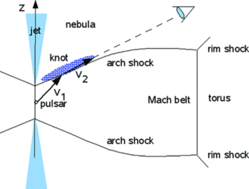
Figure 1: Interpretation of the inner knot as a highly oblique part of the termination shock (Komissarov & Lyutikov, 2011).

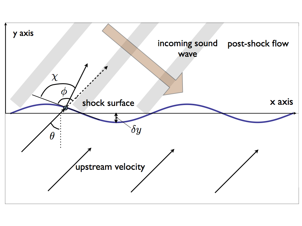
Figure 2: Geometry of the model. Initially the termination shock is an oblique planar shock, so that the incoming velocity makes angle $\theta$ with the shock normal. Magnetosonic waves coming from the post-shock flow induce corrugations of the shock surface (solid line). Locally, the shock is oblique, making and angle $\phi$ with respect to the upstream velocity. The post-shock flow makes an angle $\chi$ with respect to the initial velocity (the post-shock flow is not orthogonal to the shock plane).

2.1 Theoretical outline

The PWN can be considered a resonator with internal frequencies of the order of the fast mode travel time trough the nebular. The resonator will support normal modes with the wave length $\sim 1/L$, the size of the nebular and frequencies $\nu\sim c/L\sim$ months-years. As normal modes propagating in the shocked flow fall onto the termination shock, they will be reflected back into the post-shock medium (the reflection angle is not equal the incoming angle, the reflected amplitude may be damped or amplified). During the reflection, the waves distort the shape of the termination shock, which becomes corrugated, see Fig. 2.

Studying the corrugation perturbations of shock is an important topic in modern fluid dynamics (Landau & Lifshitz, 1959; Fowles & Houwing, 1984). Barring the spontaneous emission of waves by the shock the shock corrugation can be calculated as a reflection of the sound waves by the shock back into downstream medium. What we are interested in here is the non-resonant response of a shock to a sound wave impinging from the shocked plasma side. That is, we are looking not for normal modes of shock oscillations, but for a response of the shock to arbitrary, non-resonant perturbation.

Since the reflected waves intensity depends on the relative phase of the incoming waves and the corrugation waves, the corresponding perturbations of the downstream medium will include an entropy wave and one cannot use the barotropic equation of state; this complicates the problem considerably (Courant & Friedrichs, 1948, §73). Still, the salient features of the interaction can be derived in the limit of small amplitude of corrugation, in which case the entropy wave is weak (Courant & Friedrichs, 1948, §73). In the isentropic limit, the shock acts as a partially reflecting surface (Landau & Lifshitz, 1959, §91), with the angle of reflection not equal the incidence angle. The incident and the reflected wave then form an interference pattern in the shocked fluid. Propagation of the shock through this interference pattern then induces weaker shock corrugations.

As a simpler estimate we next consider the post-shock flow from a given corrugated shape of the shock, without calculating the dependence of the corrugation on the amplitude of the perturbing wave and neglecting the the entropy wave. General conditions at relativistic oblique perpendicular MHD shocks are considered in Appendix A.

Let us next assume that for the unperturbed oblique shock the angle of attack is $\theta$, see Fig. 2. In addition, a wave propagating from the downstream induces shock corrugations, so that in the frame of the shock surface is located at $y=\delta y\cos kx$, where $\delta y$ is the amplitude of the corrugation and $k$ is the wave number of corrugation waves propagating in $x$ direction; the upstream flow is along $y$ direction. The angle of attack at point $x$ is then

$$\cos\phi={\cos\theta+\Delta\sin kx\sin\theta\over\sqrt{1+(\Delta\sin kx)^{2}}}$$ (1)

where $\Delta=k\delta y$ is dimensionless amplitude of corrugations. Using the oblique shock conditions (A9-A15) we can then calculate the post-shock velocity and the deflection angle, see Fig. 3. The maximum post-shock velocity is reached at wave phase $\pi/2$ and equals

$$u_{2,max}=\sqrt{\frac{9\left(\Delta^{2}+1\right)}{8(\sin\theta-\Delta\cos\theta)^{2}}-1}$$ (2)

This value can be much larger than the initial unperturbed post-shock momentum, $\Delta=0$, $u_{2,0}=\sqrt{9/(8\sin^{2}\theta)-1}$. For mild amplitudes of corrugation, $\Delta\leq 1$, the post-shock velocity is especially high for highly oblique shocks, $\theta\approx\Delta$.

These estimates demonstrate that even for fluid oblique shocks, which have substantially non-relativistic post-shock velocity for normal shocks, oblique corrugated shocks can have at specific phases very high post-shock velocities. Flows with higher magnetization have even higher post-shock velocities, Fig. 4.

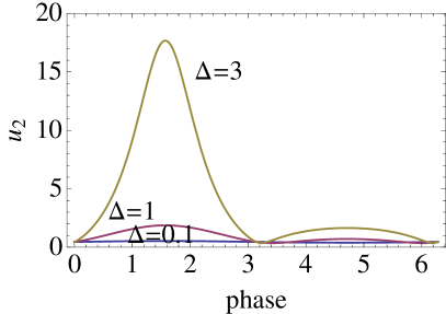
Figure 3: Deflection angle $\chi$ (left panel) and post-shock momentum $u_{1}$ (right panel) as a function of the phase of the perturbing wave for fluid shocks $\sigma=0$ for different wave amplitudes $\Delta=0.1,1,3$. The initial obliquity angle is $\theta=75^{\circ}$. For sufficiently high amplitudes a given deflection angle can be achieved up to four times per period.

Figure 4: Post-shock momentum $u_{1}$ as a function of the phase for different magnetization parameter $\sigma=0,0.1,1$ and wave amplitudes $\Delta=1$.

3 Simulations

In §3.1 we describe the numerical set up and the parameter range we investigated in our numerical simulations. In §3.2 we show the results of our simulations and discuss their implications.

3.1 Numerical Methods and Simulation Parameters

The simulations were run on a 480x240 zone mesh using the relativistic version of the RIEMANN code for astrophysical fluid dynamics (Balsara, 1998). While the code contains higher order effects (Balsara et al., 2009), in this application we used a second order ADER scheme along with a HLL Riemann solver and a WENO reconstruction. The upper and lower y boundaries were periodic, the right (pre-shock) x boundary were inflow, and the left (post-shock) boundary were set to produce the inflowing magneto-sonic waves.

In the relativistic version of the RIEMANN code we evolve the conserved variables with:

$$\partial_{t}\mathcal{U}+\partial_{i}\mathcal{F}^{i}=0$$ (3)

where

$$\mathcal{U}=\begin{bmatrix}\rho\\ \mathbf{S}_{j}\\ U\end{bmatrix},\mathcal{F}^{i}=\begin{bmatrix}\boldsymbol{v}^{i}\rho\\ \mathbf{W}^{i}_{j}\\ \mathbf{S}^{i}\end{bmatrix}$$ (4)

and

$$\mathbf{W}^{i}_{j}=\rho h\gamma^{2}\boldsymbol{v}^{i}\boldsymbol{v}_{j}-\boldsymbol{E}^{i}\boldsymbol{E}_{j}-\boldsymbol{B}^{i}\boldsymbol{B}_{j}+[P+\frac{1}{2}(E^{2}+B^{2})]\delta^{i}_{j}$$ (5)

$$\mathbf{S}=\rho h\gamma^{2}\boldsymbol{v}+\boldsymbol{E}\times\boldsymbol{B}$$ (6)

$$U=\rho h\gamma^{2}-P+\frac{1}{2}(E^{2}+B^{2})$$ (7)

We use a $\Gamma$-law equation of state which gives

$$h=1+\frac{\Gamma}{\Gamma-1}\frac{P}{\rho}$$ (8)

We evolve the induction equation as

$$\partial_{t}\boldsymbol{B}^{i}+\epsilon^{i,j,k}\partial_{j}\boldsymbol{E}_{k}=0$$ (9)

with ideal MHD approximation $\boldsymbol{E}=-\boldsymbol{v}\times\boldsymbol{B}$ and the magnetic field co-located at the zone boundaries in order to preserve the $\partial_{i}\boldsymbol{B}^{i}=0$ divergence free constraint.

Here n is the Eulerian density (n=$\gamma\rho$), $\rho$ is the Lagrangian density, $\boldsymbol{v}$ is the three-velocity, $\mathbf{S}$ is the three-momentum, $\gamma$ is the lorentz factor, $\boldsymbol{E}$ and $\boldsymbol{B}$ are the electric and magnetic field vectors, P is the pressure, h is the enthalpy, $\Gamma$ is the polytropic index ($\Gamma=\frac{4}{3}$ in all our runs), and U is the energy density. All vector quantities are defined in the Eulerian frame, i.e. the rest frame of the shock. $\delta^{i}_{j}$ is the usual Kronecker delta and $\epsilon^{i,j,k}$ is the three dimensional Levi-Civita symbol.

This application studies the long-term interaction of waves with a stationary shock. We, therefore, require shocks to stay perfectly stationary on a computational mesh for long intervals of time when they are unperturbed. The theory of stationary relativistic MHD shocks is only reasonably useful because analytically exact solutions for such shocks are only obtained in the limit of vanishing pre-shock pressure. Using the exact solutions calculated using the jump conditions in Appendix A as an approximate starting point, we evolved the solution with finite but small pre-shock pressures on a very long one dimensional computational mesh. Finite pressure and discretization errors do make this shock move slowly with respect to the mesh. By running these one dimensional simulations for a very long time, we were able to quantify the speed with which the shock drifts on the long mesh. We then lorenz boosted the fluid variables into the rest frame of the shock. The resultant densities, pressures, velocities and magnetic fields in the pre- and post-shock regions for the stationary shocks have been tabulated in Table 1.

The resulting numerically stable post-shock values were used to calculate the eigenvector for the fast right-going magneto-sonic wave using the analytical procedure from(Balsara, 2001). The resulting wave was scaled so the density perturbation was a fraction of the unperturbed post-shock density, and then allowed to propagate into the shock at a 45^o angle to the shock normal. We explored a range of angles of attack ($\phi$) to test the effect of the obliqueness of the shock, and magnetization ($\sigma$) to examine the effect of the magnetic field strength in the pulsar wind. We also varied the amplitude ( $\delta\rho/{\rho_{1}}$) of the perturbing magneto-sonic waves.

Table 1 describes the primitive variables we used to set up the shocks. In all cases the frame has been rotated so that the shock is in the y-z plane, with the magnetic field in the positive z direction. The odd numbered runs had perturbation strengths of ${\delta\rho}/{\rho_{1}}=0.3$ while the even numbered runs used ${\delta\rho}/{\rho_{1}}=0.7$. Table 2 gives the parameters defined in Appendix A corresponding to these choices of primitive variables and compares the deflection angles and compression ratios calculated using the numerical code and the analytical expressions.

Table 1: Run parameters used to set up the un-perturbed shocks for our simulations. $\rho$ is the density in the Lagrangian frame of the fluid, v_x is the fluid velocity normal to the shock, v_y is the fluid velocity along the shock, and B_z is the magnetic field perpendicular to the shock normal and the velocity vector. The velocities and magnetic field are all given in the rest frame of the shock.

Run	$\rho_{0}$	vx0	vy	P0	Bz0	$\rho_{1}$	vx1	P1	Bz1
1,2	0.1118	-0.8452	0.5286	0.001	0.2878	3.8050	-0.2542	9.100	0.951
3,4	0.1047	-0.7007	0.7057	0.001	0.9363	1.720	-0.2674	1.948	2.466
5,6	0.1190	-0.3482	0.9270	0.001	1.1254	0.6680	-0.1538	0.152	2.5610
7,8	0.1144	-0.9831	0.1698	0.001	0.2946	5.011	-0.3054	16.1850	0.9510
9,10	0.1059	-0.9523	0.283	0.001	0.9468	1.9960	-0.3860	2.8140	2.3380
11,12	0.1488	-0.8937	0.4150	0.001	1.0683	1.1446	-0.4373	0.724	2.1810

Table 2: Variables describing the geometry of the un-perturbed shocks. $\phi$ is the angle of attack, $\chi$ is the deflection angle, $\sigma$ is the magnetization of the pre-shock plasma, $\eta$ is the compression ratio between the post- and pre-shock fluids, and $\gamma_{0,1}$ are the Lorentz factors for the pre- and post-shock plasmas respectively. The table also compares the deflection angles $\chi_{num}$ and compression ratios $\eta_{num}$calculated using the numerical code and the analytical expressions, $\chi_{an}$ and $\eta_{an}$, calculated using Appendix A.

Run	$\phi$	$\chi_{num}$	$\chi_{an}$	$\sigma$	$\eta_{num}$	$\eta_{an}$	$\gamma_{0}$	$\gamma_{1}$
1,2	57.9776o	32.2950o	32.1166o	0.0046	32.2458	33.850	12.6806	1.2347
3,4	44.7963o	24.0439o	24.0094o	0.0922	16.4279	16.359	9.5316	1.5241
5,6	20.5872o	11.1670o	11.052o	0.2068	5.6134	5.474	7.1745	2.9233
7,8	80.2006o	19.2743o	19.324o	0.0036	43.8024	44.1785	14.6140	1.0673
9,10	73.4494o	19.6968o	19.7816o	0.1103	18.8480	19.042	8.7586	1.1390
11,12	65.0917o	18.5929o	19.9364o	0.2230	7.6922	10.1557	5.8646	1.2534

3.2 Simulation Results and Analysis

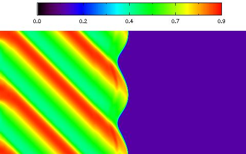
Figure 5: Density for run 5 at early time, shortly after the wave hits the shock. The corrugation wave in the shock front is especially pronounced at these early times.

Figure 6: y-velocity (transverse velocity) for Run 12 at later time. The reflected waves are interacting with the incoming waves and creating this fish-scale pattern.

Our simulations all show initially strong corrugations when the fast magneto-sonic wave first impinges on the shock. Figure 5 shows the density for our Run 5 shortly after the incoming wave has hit the shock, clearly showing the corrugation of the shock front. Larger perturbation amplitude produces more significant and persistent corrugation of the shocks. In extreme cases the perturbations could even drive the shock front off of the computational domain. These perturbations effectively constitute an extra ram-pressure term, which increases the effective post-shock pressure, moving the shock to the right. In most situations, however, the perturbations are gentle and the shocks either show a slow, secular rightward motion or none at all.

As time progresses the reflected waves coming off the shock interfere with the incoming waves, and the corrugation of the shock front begins to damp away. This damping is due to the homogenization of the effective ram pressure term as many wave fronts hit the shock. Once the simulation has stabilized we see a prominent fish-scale pattern formed by the incoming and reflected waves, with the largest variations in the fluid variables occurring at the intersections of the waves. Figure 6 provides an example of this, showing the transverse velocity in Run 12, after the reflected waves have had time to fully cross the post-shock fluid.

In all our runs we see the strongest fluctuations in the flow variables, and correspondingly the strongest variation in the observed intensity, at the early times when the shock is most deformed by the impinging magneto-sonic waves. After the shock front has had time to regain equilibrium the variation in the Lorentz factor is smaller, and we do not see the brief spikes in intensity from Doppler boosting.

4 Modeling the Gamma-ray Emission

In this section we discuss the factors responsible for the observed high energy gamma-rays in the instantaneous approximation. Later, in §5 we discuss the effect of time-of-flight considerations on the observed intensity.

The highest energy leptons emitting synchrotron radiation at $\sim 100$ MeV have a very short cooling time scale, of the order of $t_{\rm cool}\sim 10^{5}\,\gamma^{3}\,{\rm sec}$, where $\gamma$ is the bulk factor of the post-shock flow and the estimate is done for the inner wisp located at $\sim 10^{16}$ cm. Thus, we expect that only a fairly narrow region behind the shock contributes to the very high energy emission. In addition, the observed radiation is highly modulated by the relativistic beaming effects. One expects that intrinsic variations of proper emissivity have only a marginal influence on the observed flux: it is mostly dominated by Doppler boosting.

As a simple prescription that takes into account the radiative decay of shock particles and the Doppler boosting we integrate along the line of sight the quantity $\delta^{4}$ (here $\delta=1/(\gamma(1-\beta\cos\theta_{i}))$ is the Doppler factor, $\theta_{i}$ is the instantaneous angle between line of sight and the fluids velocity) for a fixed downstream distance from the shock. This is a simplified prescription that captures the two salient features of the post-shock flow: fast radiative decays and the dominant effects of relativistic Doppler boosting.

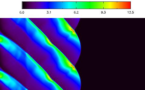
Figure 7: Synchrotron emissivity (I$\propto$P*B^α) for Run 12 at early time with $\alpha$=1.5, calculated in the fluids rest frame. The effect of the variation in this proper emissivity is expected to be negligible compared to the effects of the angle dependent Doppler boosting.

Figure 7 shows a rough estimate for the intrinsic synchrotron emissivity in Run 12, calculated using the approximation I$\propto$P*B^α, with $\alpha$=1.5 as in Jun & Jones (1999); Balsara et al. (2001). As with the other variables, we see the highest intensity in the regions around the intersection of the incoming and reflected waves. While synchrotron radiation is expected to produce the high energy gamma-rays, the effect of the line of sight dependent Doppler boosting should be the dominant term determining the observed intensity.

Figure 8: Lorentz factor for Run 6 at early time. The strong variation (a factor of 2) in the post-shock Lorentz factor leads to strong variation in the Doppler boosting along some lines of sight, which leads to spikes in the intensity.

Figure 8 shows the Lorentz factor for Run 6, which represents our most oblique parameters ($\phi=20.59^{o}$) with strongest perturbations ($\delta\rho/\rho_{1}$= 0.7). One can see that the perturbations in the post-shock flow (with unperturbed Lorentz factor $\gamma_{1}$= 2.9 ) are large, ranging from 2.09 to 3.96. This large variation in the post-shock Lorentz factor can lead to strongly enhanced observed intensity at some preferred lines of sight angles due to Doppler boosting, see Fig. 9.

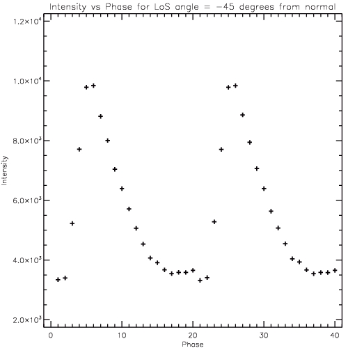
Figure 9: Calculated intensity as a function of the phase of the corrugation wave for Run 12 at early time, with the line of sight angle at -45^o to the shock normal. This profile assumes a constant rest frame emissivity, and only reflects the effect of the LoS dependent Doppler boosting ( I$\propto$$\delta^{4}$ )

In the relative intensity profiles calculated using this simple radiation model described above, we see generally broad profiles for most line of sight angles, with a few angles producing sharp peaks from small sections of the corrugation wave (Fig. 9). These peaks could be as high as twice the baseline intensity. Since the peaks are related to small segments of the shock front, they have a small characteristic time scale. These flares are most pronounced at early times of the wave-shock interaction, when the shock is strongly corrugated.

5 Time-of-flight effects: Cherenkov-type interference

The main drawback of the simplified radiation modeling described above is that it does not take into account the time-of-flight effects. One expects that neglecting the time-of-flight effects smooths out the intensity variations. We expect that the full temporal analysis will produce even sharper peaks: there is a special combination of the incoming wave direction and the amplitude of the corrugation such that the emission from the particular point of the corrugation wave add up coherently. Let us demonstrate this for a simple case of initially normal fluid shock.

Consider a wave falling from downstream onto ? relativistically strong normal shock at an angle $\alpha$ to the shock normal. In the moving fluid sound waves become dispersive. For an unperturbed fluid moving relativistically with velocity $v_{1}=1/3$ in the medium with sound speed $c_{s}=1/\sqrt{3}$, the corresponding dispersion relation (Anile, 1989, Eq. 10.18) becomes

$${\omega\over k}={\sqrt{50-2\cos 2\alpha}-3\cos\alpha\over 13}$$ (10)

The phase speed of corrugation perturbations along the shock normal is then

$$v_{ph}={\sqrt{50-2\cos 2\alpha}-3\cos\alpha\over 13\sin\alpha}$$ (11)

The corrugations become luminal for incidence angles smaller than $\alpha=0.32$. For smaller incidence angles the corrugation wave is superluminal. If a post-shock flow at some phase satisfies the Cherenkov condition

$$\sin\chi=c/v_{ph}$$ (12)

the waves emitted by this phase will add up constructively. Equation (12) together with the expression for the phase speed (11) and the post shock flow angle (A15) with $\phi=\pi/2$ defines the condition on the incidence angle of a sound wave coming from the shocked fluid, such that the resulting corrugations of the shock surface produce the post-shock flow which remains in phase with the corrugation wave. In this case the corrugation pattern acts as a real particle, emitting light at the Cherenkov condition.

6 Discussion

In this work we considered emission from a relativistic corrugated shocks. We performed relativistic simulations of the corrugations of the perpendicular MHD shocks induced by strong magnetosonic waves impinging from the downstream medium. Our main conclusions is that long wavelength perturbations with the relative amplitude of $\sim 0.5-0.7$ of the downstream density can result in sharp intensity variations, with duration of the peak much smaller than the wave period. Sharp intensity variations can have amplitudes of an order of magnitude in flux, with large modulation index, of the order of $0.5$.

Variable, mildly relativistic post-shock flow may also explain (or, in fact, be required in stochastic shock acceleration models) the very high break energy observed in the Crab flares. As argued by Lyutikov (2010) (see also de Jager et al., 1996), there is an acceleration model-independent upper limit on the frequency of synchrotron emission by radiation reaction-limited acceleration of electrons:

$$\epsilon_{\rm max}\approx\hbar{mc^{3}\over e^{2}}\approx 100\mbox{ MeV}.$$ (13)

The break energy observed by Fermi satellite in Crab’s quiescent state, $\sim 100$ MeV (Fermi Collaboration & Pulsar Timing Consortium, 2009), approaches this limit, while the break energies during flares, $\sim 500$ MeV (Tavani et al., 2011; Abdo et al., 2011), exceed it. If emission is generated in a relativistically moving plasma, the maximum observed synchrotron frequency is boosted by the Doppler factor. Note also, that previously EGRET data did indicate a moderate level of the cut-off energy variability (de Jager et al., 1996).)

Another important feature of our model is that in the proposed model the time scale of the flare is set not by the radiative decay time of the emitting particles, but by the overall dynamics of the termination shock. Thus, the flare time scale cannot be used to estimate the magnetic field within the emission region.

We would like to thank Sergey Komissarov for suggesting the possibility discussed in this paper.

Appendix A Oblique relativistic MHD shocks

We derive jump conditions at oblique relativistic perpendicular MHD shocks, when the magnetic field is orthogonal to flow velocity which is not aligned with the shock normal. We investigate the post-shock parameters as functions of the upstream plasma magnetization $\sigma$, Lorentz factor $\gamma_{1}$ and the angle of attack $\phi$. Previously, Webb et al. (1987) investigated oblique relativistic MHD shocks in the quasi-parallel case, when the planes of fluid velocity and of the magnetic field coincide. Konigl (1980) considered relativistic fluid oblique shocks. Here we consider relativistic oblique perpendicular magnetohydrodynamic shocks, so that the magnetic field is in the plane of the shock and is orthogonal to the fluid velocity. This appendix corrects an error in Lyutikov (2004).

Let the stream lines make an angle $\phi$ with the shock normal and let the post-shock flow make an angle $\chi$ with the initial velocity, Fig. 10. Normal shock corresponds to $\phi=\pi/2$.

Figure 10: Geometry of the flow

Keeping only $x$-dependence, the equations of perpendicular relativistic MHD read (e.g.,  Anile, 1989)

$$\partial_{x}\left(nu_{x}\right)=0\mbox{}$$

$$\partial_{x}\left(p+B^{2}/2+(w+B^{2})u_{x}^{2}\right)=0\mbox{}$$

$$\partial_{x}\left((w+B^{2})\gamma u_{x}\right)=0\mbox{}$$

$$\partial_{x}\left(uB\right)=0$$ (A1)

where $n$ is proper density, $w=e+p=n+\Gamma/(\Gamma-1)p$ is fluid enthalpy, $e$ is internal energy, $B$ is rest-frame magnetic fields, $u$ is a four-velocity. Note that in this Appendix we use the rest-frame magnetic field and density as primitive variables, while the numerical simulations in §3.1 use the quantities in the lab frame.

Oblique shock conditions can be obtained from normal shocks and an additional condition that the component along the shock velocity remains constant (e.g.,  Konigl, 1980; Anile, 1989):

$$n_{0}u_{0}\sin\phi=n_{1}u_{1}\sin(\phi-\chi)\mbox{}$$

$$B_{0}u_{0}\sin\phi=B_{1}u_{1}\sin(\phi-\chi)\mbox{}$$

$$p_{0}+B_{0}^{2}/2+(w_{0}+B_{0}^{2})u_{0}^{2}\sin^{2}\phi=p_{1}+B_{1}^{2}/2+(w_{1}+B_{1}^{2})u_{1}^{2}\sin^{2}(\phi-\chi)\mbox{}$$

$$(w_{0}+B_{0}^{2})\gamma_{0}u_{0}\sin\phi=(w_{1}+B_{1}^{2})\gamma_{1}u_{1}\sin(\phi-\chi)\mbox{}$$

$$\beta_{0}\cos\phi=\beta_{1}\cos(\phi-\chi)$$ (A2)

where subscripts refer to upstream ($0$) and downstream ($1$) regions and $\beta$ is three-velocity. Below we assume the relativistic equations of state with $\Gamma=4/3$.

The problem is to express the post-shock parameters ($p_{1},n_{1},B_{1},u_{1}$ and $\chi$) in terms of the upstream parameters ($p_{0},n_{0},B_{0},u_{0}$ and $\phi$). As we demonstrate below, the corresponding equation take especially simple form is expressed in terms of the compression ratio $\eta=n_{1}/n_{0}$, which in turn depends on the upstream parameters. By ideal condition $B_{1}=\eta B_{0}$. Compression ratio can be related to the turning angle $\chi$

$$\eta^{2}=\left(1+u_{0}^{2}\sin^{2}\phi-\gamma_{0}^{2}\sin^{2}(\phi-\chi)\right){\tan^{2}\phi\over\sin^{2}(\phi-\chi)}$$ (A3)

In term of $\eta$,

$$u_{0}^{2}\sin^{2}\phi={\left((p_{1}-p_{0})+(B_{1}^{2}-B_{0}^{2})/2\right)\eta^{2}\over\eta^{2}(w_{0}+B_{0}^{2})-(w_{1}+B_{1}^{2})}\mbox{}$$

$$u_{1}\sin^{2}(\phi-\chi)={\left((p_{1}-p_{0})+(B_{1}^{2}-B_{0}^{2})/2\right)\eta^{2}\over\eta^{2}(w_{0}+B_{0}^{2})-(w_{1}+B_{1}^{2})}\mbox{}$$

$$u_{1}^{2}={u_{0}^{2}\over\eta^{2}}{\sin^{2}\phi\over\sin^{2}(\phi-\chi)}={\eta^{2}\cos^{2}\phi+\gamma_{0}^{2}\sin^{2}\phi\over\eta(1+u_{0}^{2}\sin^{2}\phi}\mbox{}$$

$$\sin^{2}(\phi-\chi)={\sin^{2}\phi\over\eta^{2}\cos^{2}\phi+\sin^{2}\phi}$$ (A4)

Introducing magnetization parameter $\sigma=B_{0}^{2}/w_{0}$, the jump conditions (A2) can be resolved for post-shock pressure $p_{1}$ and enthalpy $w_{1}$ as functions of $\eta$:

$$p_{1}=p_{0}-{w_{0}\sigma(\eta^{2}-1)\over 2}+u_{0}^{2}w_{0}\sin^{2}\phi(1+\sigma)\left(1-\sqrt{1+u_{0}^{2}\sin^{2}\phi\over\eta^{2}+u_{0}^{2}\sin^{2}\phi}\right)\mbox{}$$

$$w_{1}=w_{0}\eta^{2}\left(-\sigma+(1+\sigma)\sqrt{1+u_{0}^{2}\sin^{2}\phi\over\eta^{2}+u_{0}^{2}\sin^{2}\phi}\right)$$ (A5)

In case of cold plasma, $p_{0}=0$ the compression ratio $\eta$ can then be simply related to the inflow parameters:

$$\eta^{2}\left((\sigma+1)\sqrt{\frac{u_{0}^{2}\sin^{2}\phi+1}{u_{0}^{2}\sin^{2}\phi+\eta^{2}}}+\sigma\right)+4u_{0}^{2}(\sigma+1)\sin^{2}\phi\left(\sqrt{\frac{u_{0}^{2}\sin^{2}\phi+1}{u_{0}^{2}\sin^{2}\phi+\eta^{2}}}-1\right)-\eta-2\sigma=0$$ (A6)

Let us next simplify the above relations in the high compression limit, $\eta\rightarrow\infty$. (The strong compression limit becomes inapplicable for $\sin\phi\leq 1/(u_{0}\sqrt{1+\sigma})$.) Eq. (A6) gives

$${\eta^{2}\over u_{0}^{2}}=\frac{16(1+\sigma)\sin^{2}\phi}{8\sigma^{2}+2\left(\sqrt{16\sigma^{2}+161+\sigma}+5\right)\sigma+\sqrt{16\sigma^{2}+16\sigma+1}+1}\approx\left\{\begin{array}[]{cc}8(1-9\sigma)\sin^{2}\phi,&\sigma\ll 1\\ {1\sin^{2}\phi\over\sigma},&\sigma\gg 1\end{array}\right.$$ (A7)

The turning angle is given by

$$\tan\chi={(1-{\cal Z})\cos\phi\sin\phi\over\cos^{2}\phi+{\cal Z}\sin^{2}\phi}\mbox{}$$

$${\cal Z}=\sqrt{\frac{8\sigma^{2}+2\left(\sqrt{16\sigma^{2}+16\sigma+1}+5\right)\sigma+\sqrt{16\sigma^{2}+16\sigma+1}+1}{8\sigma^{2}+2\left(\sqrt{16\sigma^{2}+16\sigma+1}+13\right)\sigma+\sqrt{16\sigma^{2}+16\sigma+1}+17}},\,1/3<{\cal Z}<1$$ (A8)

Maximum deflection angle is reached at $\cos\phi=\sqrt{{\cal Z}/(1+{\cal Z}}$ and equals $\tan\chi_{max}=(1-{\cal Z})/(2{\cal Z})=1/2(\tan\phi-\cot\phi)$, Fig. 11.

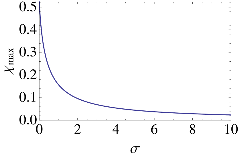
Figure 11: Maximum deflection angle $\chi_{max}$ as a function of the magnetization parameters $\sigma$ in the limit $u_{0}^{2}\rightarrow\infty$. $\chi_{max}=\pi/6$ for $\sigma=0$, $\chi_{max}\approx 1/(4\sigma)$ for $\sigma\gg 1$.

The post-shock four-velocity

$$u_{1}^{2}\sin^{2}\phi=\frac{1}{8}\left(9-8\sin^{2}\phi\right)+\frac{8\sigma^{2}+2\left(\sqrt{16\sigma^{2}+16\sigma+1}+4\right)\sigma+\sqrt{16\sigma^{2}+16\sigma+1}-1}{16(\sigma+1)}$$ (A9)

(for normal shock, $\phi=\pi/2$, Eq. (A9) reproduces Eq. (4.11) of Kennel & Coroniti, 1984), see Fig. 12.

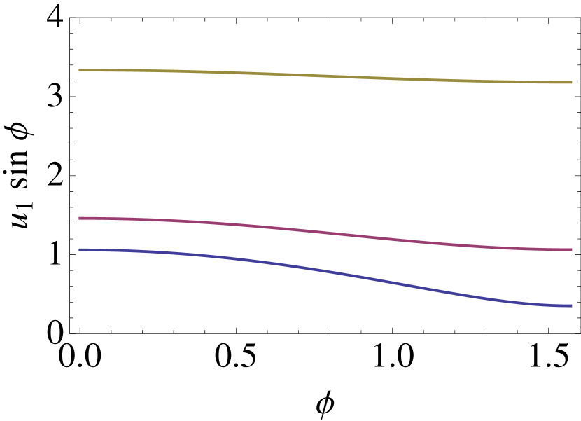
Figure 12: Dependence of $u_{1}\sin\phi$ (the post-shock four-velocity times angle of attack) the angle of attack $\phi$ for different magnetization parameters $\sigma=0,1,10$ (bottom to top).

In the high $\sigma$ limit, $u_{1}^{2}\sin^{2}\phi\approx\sigma+(9/8-\sin^{2}\phi)+{\cal O}(1/\sigma)$.

Using the post-shock fast velocity (Harris, 1957)

$$c_{f}^{2}={B_{1}^{2}+4/3p_{1}\over B_{1}^{2}+4p_{1}+n_{1}},$$ (A10)

the post-shock Mach number is

$$M_{1}^{2}={v_{1}^{2}\over c_{f}^{2}}=\frac{3({\cal Z}+1)\left(\left({\cal Z}^{2}-1\right)\sin^{2}\phi+1\right)}{7{\cal Z}-1}\approx\mbox{}$$

$$\left\{\begin{array}[]{ll}\frac{1}{3}+\frac{8\cos^{2}\phi}{3}+\left(\frac{2}{3}-\frac{56\cos^{2}\phi}{3}\right)\sigma,&\sigma\ll 1\\ 1+\frac{\cos^{2}\phi-{2}/{3}}{\sigma},&\sigma\gg 1\end{array}\right.$$ (A13)

The flow becomes supersonic for

$$\cos 2\phi<\frac{3{\cal Z}^{2}+6{\cal Z}-5}{3({\cal Z}+1)^{2}}$$ (A14)

(see Fig. 13).

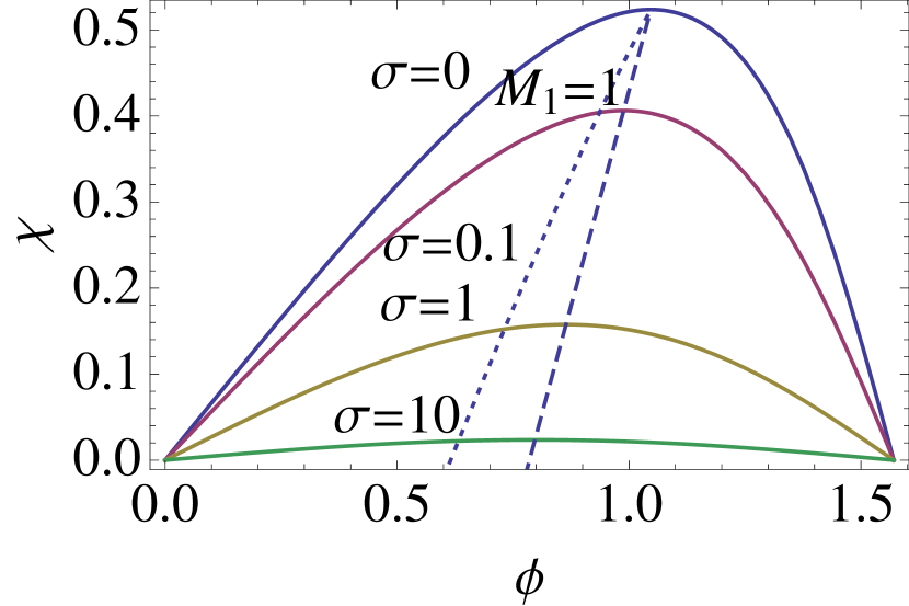
Figure 13: Dependence of the deflection angle $\chi$ on the angle of attack $\phi$ for different magnetization parameters $\sigma$ in the limit $u_{0}^{2}\rightarrow\infty$, . Dotted line is $M_{1}=1$ line, Eq. (A14); dashed line is the line of maximum deflection $\tan\chi_{max}=1/2(\tan\phi-\cot\phi)$.

In particular, for strong fluid shocks, $\sigma=0$, in the limit of high compression ratio, $\eta\gg 1$,

$$\eta^{2}=8u_{0}^{2}\sin^{2}\phi\mbox{}$$

$$u_{1}^{2}={9\over 8\sin^{2}\phi}-1\mbox{}$$

$$\tan\chi={\sin 2\phi\over 2+\cos 2\phi}$$ (A15)

Maximum deflection is reached at $\phi=\pi/3$ and is equal to $\chi=\pi/6$ (Konigl, 1980). In the large compression limit the post-shock Mach number is

$$M_{1}^{2}={3-(8/3)\sin^{2}\phi}$$ (A16)

The flow becomes sonic at the maximum turning angle $\phi=\pi/3$.

References

- Abdo et al. (2011) Abdo, A. A., Ackermann, M., Ajello, M., Allafort, A., Baldini, L., Ballet, J., Barbiellini, G., Bastieri, D., Bechtol, K., Bellazzini, R., Berenji, B., Blandford, R. D., Bloom, E. D., Bonamente, E., Borgland, A. W., Bouvier, A., Brandt, T. J., Bregeon, J., Brez, A., Brigida, M., Bruel, P., Buehler, R., Buson, S., Caliandro, G. A., Cameron, R. A., Cannon, A., Caraveo, P. A., Casandjian, J. M., Çelik, Ö., Charles, E., Chekhtman, A., Cheung, C. C., Chiang, J., Ciprini, S., Claus, R., Cohen-Tanugi, J., Costamante, L., Cutini, S., D’Ammando, F., Dermer, C. D., de Angelis, A., de Luca, A., de Palma, F., Digel, S. W., do Couto e Silva, E., Drell, P. S., Drlica-Wagner, A., Dubois, R., Dumora, D., Favuzzi, C., Fegan, S. J., Ferrara, E. C., Focke, W. B., Fortin, P., Frailis, M., Fukazawa, Y., Funk, S., Fusco, P., Gargano, F., Gasparrini, D., Gehrels, N., Germani, S., Giglietto, N., Giordano, F., Giroletti, M., Glanzman, T., Godfrey, G., Grenier, I. A., Grondin, M.-H., Grove, J. E., Guiriec, S., Hadasch, D., Hanabata, Y., Harding, A. K., Hayashi, K., Hayashida, M., Hays, E., Horan, D., Itoh, R., Jóhannesson, G., Johnson, A. S., Johnson, T. J., Khangulyan, D., Kamae, T., Katagiri, H., Kataoka, J., Kerr, M., Knödlseder, J., Kuss, M., Lande, J., Latronico, L., Lee, S.-H., Lemoine-Goumard, M., Longo, F., Loparco, F., Lubrano, P., Madejski, G. M., Makeev, A., Marelli, M., Mazziotta, M. N., McEnery, J. E., Michelson, P. F., Mitthumsiri, W., Mizuno, T., Moiseev, A. A., Monte, C., Monzani, M. E., Morselli, A., Moskalenko, I. V., Murgia, S., Nakamori, T., Naumann-Godo, M., Nolan, P. L., Norris, J. P., Nuss, E., Ohsugi, T., Okumura, A., Omodei, N., Ormes, J. F., Ozaki, M., Paneque, D., Parent, D., Pelassa, V., Pepe, M., Pesce-Rollins, M., Pierbattista, M., Piron, F., Porter, T. A., Rainò, S., Rando, R., Ray, P. S., Razzano, M., Reimer, A., Reimer, O., Reposeur, T., Ritz, S., Romani, R. W., Sadrozinski, H. F.-W., Sanchez, D., Parkinson, P. M. S., Scargle, J. D., Schalk, T. L., Sgrò, C., Siskind, E. J., Smith, P. D., Spandre, G., Spinelli, P., Strickman, M. S., Suson, D. J., Takahashi, H., Takahashi, T., Tanaka, T., Thayer, J. B., Thompson, D. J., Tibaldo, L., Torres, D. F., Tosti, G., Tramacere, A., Troja, E., Uchiyama, Y., Vandenbroucke, J., Vasileiou, V., Vianello, G., Vitale, V., Wang, P., Wood, K. S., Yang, Z., & Ziegler, M. 2011, Science, 331, 739
- Anile (1989) Anile, A. M. 1989, Relativistic fluids and magneto-fluids: With applications in astrophysics and plasma physics, ed. Anile, A. M.
- Balsara (1998) Balsara, D. 1998, The Astrophysical Journal Supplement Series, 116, 119
- Balsara (2001) —. 2001, The Astrophysical Journal Supplement Series, 132, 83
- Balsara et al. (2001) Balsara, D., Benjamin, R., & Cox, D. 2001, The Astrophysical Journal, 563, 800
- Balsara et al. (2009) Balsara, D., Rumpf, T., Dumbser, M., & Munz, C.-D. 2009, Journal of Computational Physics, 228, 2480
- Bednarek & Idec (2010) Bednarek, W., & Idec, W. 2010, ArXiv e-prints 1011.4176
- Bucciantini & Del Zanna (2006) Bucciantini, N., & Del Zanna, L. 2006, A&A, 454, 393
- Camus et al. (2009) Camus, N. F., Komissarov, S. S., Bucciantini, N., & Hughes, P. A. 2009, MNRAS, 400, 1241
- Courant & Friedrichs (1948) Courant, R., & Friedrichs, K. O. 1948, Supersonic flow and shock waves, ed. Courant, R. & Friedrichs, K. O.
- de Jager et al. (1996) de Jager, O. C., Harding, A. K., Michelson, P. F., Nel, H. I., Nolan, P. L., Sreekumar, P., & Thompson, D. J. 1996, ApJ, 457, 253
- D’yakov (1954) D’yakov, S. P. 1954, JETP, 27, 288
- Fermi Collaboration & Pulsar Timing Consortium (2009) Fermi Collaboration, & Pulsar Timing Consortium, F. 2009, ArXiv e-prints
- Fowles & Houwing (1984) Fowles, G. R., & Houwing, A. F. P. 1984, Physics of Fluids, 27, 1982
- Harris (1957) Harris, E. G. 1957, Physical Review, 108, 1357
- Hester (2008) Hester, J. J. 2008, ARA&A, 46, 127
- Jun & Jones (1999) Jun, B.-I., & Jones , T. W. 1999, The Astrophysical Journal, 511, 774
- Kennel & Coroniti (1984) Kennel, C. F., & Coroniti, F. V. 1984, ApJ, 283, 694
- Komissarov & Lyubarsky (2004) Komissarov, S. S., & Lyubarsky, Y. E. 2004, MNRAS, 349, 779