Nonparametric Link Prediction in Large Scale Dynamic Networks
Abstract
We propose a nonparametric approach to link prediction in large-scale dynamic networks. Our model uses graph-based features of pairs of nodes as well as those of their local neighborhoods to predict whether those nodes will be linked at each time step. The model allows for different types of evolution in different parts of the graph (e.g, growing or shrinking communities). We focus on large-scale graphs and present an implementation of our model that makes use of locality-sensitive hashing to allow it to be scaled to large problems. Experiments with simulated data as well as five real-world dynamic graphs show that we outperform the state of the art, especially when sharp fluctuations or nonlinearities are present. We also establish theoretical properties of our estimator, in particular consistency and weak convergence, the latter making use of an elaboration of Stein’s method for dependency graphs.
1 Introduction
Many real-world problem domains generate data in the form of graphs or networks. Examples include social networks (e.g., Facebook), recommendation services (e.g., Netflix or Last.fm), biochemical networks, citation graphs and market analysis. The inferential problem in these settings is often one of link prediction. This problem can be formulated in a static setting where one assumes that a fixed but unknown graph is partially observed, and one wishes to assess whether a pair of nodes that are not known to be linked are in fact linked, given an observed linkage pattern among other nodes. Many real-world graphs are often best modeled, however, as dynamic entities, where links can arise and disappear over time. In the dynamic setting the link prediction problem involves assessing whether two nodes will be linked at time given the linkage patterns at all previous times.
Real-world graphs of current interest are often very large, involving many hundreds of thousands or millions of nodes. The dynamic setting involves sequences of such graphs. Given the large-scale nature of these data structures, inferential methodology that may be feasible on smaller graphs of hundreds of nodes, such as Markov random fields and other graphical models, are generally infeasible for real-world link prediction problems, and practical approaches to such problems generally involve simple heuristics, such as estimating a probability of a link being present as a simple function of the last time a pair of nodes formed a link, or the number of common neighbors between a pair of nodes [12, 17, 27, 30]. While these heuristics do respect the computational imperative, and are often useful in practice, there has been little in the way of statistical analysis to provide a sound foundation for their use and to assess the quality of the inferences that they provide. This is particularly true in the dynamic setting, where link prediction is often approached by specifying various measures of connectivity in a static graph and extending these measures in an ad hoc manner to sequences of graphs.
In this paper, we develop a nonparametric methodology for link prediction in large-scale dynamic networks. Our methodology is a relatively simple kernel-based approach, one that aims to retain the virtues of the simple heuristic methods, both in their favorable computational scaling and in the relatively weak assumptions that they appear to make on the graph generation process. As compared to existing heuristic approaches, however, our kernel-based approach allows us to provide a formal inferential treatment of link prediction—we establish consistency and weak convergence of our estimator. On the computational front, while a naive implementation of a kernel method would have poor scaling (due to the need to compare query points to every point in a training set), we show that our kernel-based approach is amenable to locality sensitive hashing (LSH) [13], which provides a fast and scalable implementation of the estimator.
Our approach is in the spirit of the nonparametric autoregressive time series models [18]. In these models the evolution of a sequence of continuous univariate random variables is modeled by taking the conditional expectation of to be a function of a moving window , and estimating this function via kernel regression. It is also possible to consider multivariate extensions of such models. While it would be possible in principle to apply such models to our problem by encoding graphs as vectors, in practice the large-scale graphs that are our focus would generate high-dimensional vector representations that would be fatal to naive kernel regression. Instead, we think of the graphs as providing a “spatial” dimension that is orthogonal to the time axis. In addition to imposing the conditional independence assumption implicit in the use of a moving window, we make the additional assumption that the linkage behavior of any node is independent of the rest of the graph given its “local neighborhood”; in effect, local neighborhoods are to the spatial dimension what moving windows are to the time dimension.
Thus we model the out-edges of at time as a function of the local neighborhood of over a moving window of time, resulting in a much more tractable problem. As a byproduct, this also allows for different evolutions for different regions to exist in the same graph; e.g., regions of slow versus fast change in links, assortative versus disassortative regions (where high-degree nodes are more/less likely to connect to other high-degree nodes), densifying versus sparsifying regions, and so on.
As a brief summary, our contributions are as follows:
(1) Nonparametric problem formulation: We offer, to our
knowledge, the first nonparametric model for link prediction in dynamic networks.
The model is powerful enough to accommodate different regions with different dynamics,
which is not accommodated in existing heuristic approaches. It also allows covariates
to be incorporated (such as demographic data about a node).
(2) Consistency and weak convergence of the estimator: We prove consistency of our estimator using notions of strong mixing in Markov chains. To establish weak convergence we show how to adapt Stein’s method to our setting, going beyond the dependency graph formulation of Stein’s method [25] to allow long-range weak dependence instead of marginal independence.
(3) Fast implementation via LSH: Nonparametric methods such as kernel regression require computing kernel similarities between a query and all members of the training set. A naive implementation would lead to computation linear in the training set size, which is generally infeasible for large-scale networks. In order to mitigate this issue, we adapt the locality sensitive hashing algorithm of Indyk and Motwani [13] to our particular kernel function.
(4) Empirical improvements over previous methods: We demonstrate the empirical effectiveness of our method on link prediction tasks on both simulated and real networks. On graphs with nonlinear linkage patterns (e.g., seasonal trends), we outperform all of the state-of-the-art heuristic measures for static and dynamic graphs. This result is obtained in particular on a real-world sensor network graph. On other real-world datasets with smoother and simpler evolution, we perform as well as the best competitor. Finally, we compare our LSH-based kernel regression to exact kernel regression, and show that the LSH-based approach yields almost identical accuracy at a fraction of the computational cost.
The rest of the paper is organized as follows. We present the model and the estimator in Section 2. Our LSH implementation is described in Section 3. Section 4 provides an experimental evaluation of our method. We provide an analysis of consistency in 5. In Section 6 we discuss our adaptation of Stein’s method which we use to establish weak convergence of our estimator in Section 7. We provide a discussion of related work in Section 8 and we present our conclusions in Section 9.
2 The Model and the Estimator
We begin by introducing some notation. Consider a sequence of directed graphs, . Define the indicator which equals if the edge exists at time , and otherwise. Let denote the local neighborhood of node in ; in our experiments, we define it to be the set of nodes within two hops of and all edges between the nodes in that set. Note that the neighborhoods of nearby nodes can overlap. Let ; this represents the local neighborhood of along both spatial and temporal dimensions.
2.1 The Model
Our model is as follows:
where is a function of two sets of features: those specific to the pair of nodes under consideration——and those for the local neighborhood of the endpoint —. We require that both of these feature sets be functions of . Thus, is assumed to be independent of given , limiting the dimensionality of the problem. Note that two pairs of nodes and that are close to each other in terms of graph distance are likely to have overlapping neighborhoods, and hence a higher probability of sharing neighborhood-specific features. Thus, link prediction probabilities for pairs of nodes from the same region are likely to be similar, as desired.
To make this statement precise, we will need to impose smoothness properties on . We will show that given appropriate assumptions of smoothness (Assumption 1 in Section 5), nonparametric kernel estimators have desirable consistency properties.
Assume that the pair-specific features come from a finite set ; if not, they are discretized into such a set. For example, one may let record the number of common neighbors between and and the last time a link appeared between these nodes (lastlink); note that both are functions of . Let , where are the number of node pairs in with feature vector , and the number of such pairs which were also linked by an edge in the next timestep . In a nutshell, tells us the chances of an edge being created in given its features in , averaged over the whole neighborhood —in other words, it captures the change of the neighborhood around over one timestep.
One can think of as a contingency table indexed by the features . Contingency tables are widely referred to as “datacubes” in the database community, and we will adopt this terminology, refering to as a datacube, and a feature vector as the “cell” in the datacube with contents . Finiteness of is necessary to ensure that datacubes are finite-dimensional, which allows us to index them and quickly find nearest-neighbor datacubes.
2.2 The Estimator
Our estimator of the function at time is:
| (1) |
where we factor the kernel function into neighborhood-specific and pair-specific parts: . Let denote the distance between features and , and let denote the set of features at distance from feature . We define as
| (2) |
where is a bandwidth parameter which we will require to be for some in order to obtain consistency and distributional convergence. is a discrete analog of a continuous kernel function (similar functions can be found in Aitchison and Aitken [2] and Wang and van Ryzin [32]). As is the case with continuous kernel functions, it has the property that as the bandwidth parameter , it is equal to one if and only if , and zero otherwise. Similarly has the property that as , it approaches . This inner kernel function can also be extended to features at distance two and so forth, while weighing those terms by powers of .
Plugging in the definition of the kernel in Equation 1, we obtain the following interpretation of the estimator:
| (3) |
Useful intuition can be obtained by considering the case . Here, given the query pair at time , we look inside cells for the query feature in all neighborhood datacubes, compute the average and in these cells after accounting for the similarities of the datacubes to the query neighborhood datacube, and use their quotient as the estimate of linkage probability. Letting provides an estimator that deals more effectively with sparsity by computing weighted averages of and over features that are “close” to .
Thus, the probability estimates are derived from historical instances where (a) the feature vector of the historical node pair matches the query, and (b) the local neighborhood is similar as well.
Now, we need a measure of the similarity between neighborhoods, with the goal of treating two neighborhoods as similar if they have similar probabilities of generating links between node pairs with feature vector , for any . To this end we could simply compare point estimates , but we also wish to account for the variance in these estimates. We achieve this by defining a similarity measure that has a Bayesian flavor:
| (4) | |||||
where denotes the total variation distance between the distributions of and , is the beta distribution and is a bandwidth parameter. We will require for some to obtain appropriate rates when we study the consistency and distributional convergence of our estimator.
Remarks. To better understand our choice of estimator, consider by way of contrast a simple estimator that computes the fraction of pairs for which the feature lastlink was equal to at time and which formed an edge at time (for ). This approach suffers from two key problems that make it perform poorly on real-world graphs. First, it does not allow for local variations in the link-formation fractions, as would be expected for communities evolving differently within the same graph. We address this problem by maintaining a separate datacube for each local neighborhood. The second, more subtle, problem is the implicit assumption of stationarity—a node’s link-formation probabilities are assumed to be time-invariant functions of the datacube features. This assumption does not allow for seasonal changes in linkage patterns, or for a transition from slow to fast growth, etc. Our model addresses this issue by finding historical neighborhoods from some previous time with datacubes similar to the query datacube, and uses their evolution from to to predict link formation in the next time step for the current neighborhood. This helps us learn nonlinear trends.
Our estimator also has the virtue that it combats sparsity by aggregating data across similarly-evolving communities even if they are separated by graph distance and time. That said, sparsity remains a serious issue, and we provide a further discussion of sparsity in the following section.
Finally, note that we build the datacube so as to encode the recent change of a neighborhood, and not just the distribution of features in the neighborhood. Thus, for example, two neighborhoods may have the same datacube if the fraction of node pairs that formed an edge in the next timestep is the same in both neighborhoods, and not if they both merely had the same number of pairs. Thus, it is the change in link structure that drives the estimation of linkage probabilities. Moreover, two neighboring nodes may end up having very similar datacubes, and will end up forming links in a similar way, whereas very different datacubes will reflect the variations in link formation patterns among different communities.
2.3 Sparsity
For sparse graphs, or short time series, two practical problems can arise. First, a node can have zero degree and hence an empty neighborhood. To cope with this issue, we define the neighborhood of node as the union of two-hop neighborhoods over the last timesteps. Second, and more problematically, the and values obtained from kernel regression can be small, yielding an estimated linkage probability that is unreliable numerically.
We offer a threefold solution to this problem, the first element of which is already present in our estimator. (a) The inner kernel (Equation 2) combines and with a weighted average of the corresponding values for any that are “close” to , the weights encoding the similarity between and . (b) In determining a final ranking, instead of using directly, we use the lower end of the Wilson score interval [33]. The node pairs that are ranked highest according to this “Wilson score” are those that have high estimated linkage probability and is high (implying a reliable estimate). (c) We use a “backoff” smoothing procedure for the Wilson scores, in which the raw scores are smoothed against the scores obtained from a “prior” datacube, which is the average of all historical datacubes. The degree of smoothing depends on . This can be thought of as a simple hierarchical model, where the lower level (set of individual datacubes) smooths its estimates using the higher level (the prior datacube).
3 Fast search using LSH
A naive implementation of the nonparametric estimator in Equation (3) computes kernel similarity between the query datacube and all datacubes for each of the timesteps for each prediction, which can be infeasibly slow for large graphs. To obtain a more computationally tractable estimator, we consider only the top- closest neighborhoods (in terms of the largest kernel similarities). The value of is a parameter of the algorithm; for our experiments we use . What is needed to make this practical is a fast method (one that runs in sublinear time) to quickly find the top- closest neighborhoods.
We achieve this by using locality sensitive hashing (LSH) [13]. Hashing is often used in databases for fast “table-lookups” or retrieving matching items from a large database. The key component is a hash function that maps a given “key” or object to a certain hash value. In order to search for a particular key, we compute the hash value and do a table lookup with this value. The concept of “locality sensitive” hashing refers to hash functions having the property that, with high probability, two “similar” data items are hashed to the same value. This facilitates approximate nearest neighbor search, and is suitable for high-dimensional spaces, where traditional nearest neighbor search techniques are often infeasible.
The standard LSH method operates on bit sequences, and maps sequences with small Hamming distance to the same hash bucket. In our setting, we must hash datacubes, and use the total variation distance metric. We make use of the fact that total variation distance between discrete distributions is half the distance between the corresponding probability mass functions. If we could approximate the probability distributions in each datacube cell with bit sequences, then the distance would just be the Hamming distance between these sequences, making our setting amenable to the use of standard LSH. We achieve this with three steps:
- Conversion to bit sequence
-
The key idea is to approximate the linkage probability distribution by discretization. We first discretize the range (since we deal with probabilities) into buckets. For each bucket we compute the probability mass falling inside it. This is encoded using bits by setting the first bits to 1, and the others to 0. In this way the entire distribution (i.e., one cell) is represented by bits. As a result the entire datacube can now be stored in bits. However, in all our experiments, datacubes were very sparse with only cells ever being non-empty (usually, 10-50); thus, we use only bits in practice. The Hamming distance between two pairs of bit vectors yields the total variation distance between datacubes (modulo a constant factor).
- Distances via LSH
-
We create a hash function by picking a uniformly random sample of bits out of . For each hash function, a hash table is created to store all datacubes whose hashes are identical in these bits. We use such hash functions. A query datacube is first hashed using each of these functions. Then we create a candidate set containing of distinct datacubes sharing any of these hashes. The total variation distance of these candidates to the query datacube is computed explicitly, yielding the closest matching historical datacubes.
- Picking
-
The number of bits is crucial in balancing accuracy versus query time: while a large hashes all datacubes to their own hash bucket, returning a few or no matches to the query, a small bunches many datacubes into the same bucket, decreasing the probability of finding the ‘true’ near neighbors. In the spirit of Indyk and Motwani [13], we do a binary search to find the for which the average hash-bucket size over a query workload is just enough to provide the desired top- matches. We evaluate the accuracy of this approach in Section 4.
We conclude this section with two additional points. First, we never create the entire bit representation of bits explicitly; only the hashes need to be computed, taking time. Second, the main cost in the algorithm is in creating the hash table, which needs to be done once as a preprocessing step. Query processing is extremely fast and sublinear, since the candidate set is much smaller than the size of the training set.
4 Experiments
We start by introducing several baseline algorithms, and our evaluation metric. These baselines were picked carefully from previous work as being those that have yielded state-of-the-art performance in a range of link prediction tasks. In our first set of experiments we use simulated data to compare the performance of our algorithm to these baselines, focusing on situations involving seasonality in link formation. Second, we study the performance of our algorithm and the baselines on several real-world graphs: a sensor network, two co-authorship graphs, and a graph of Facebook employees. Finally, we investigate the computational scaling of our approach, comparing the improvement in runtime of the LSH-based algorithm to an exact algorithm, and investigating the effect of the LSH bit-size on accuracy.
4.1 Baselines and metrics
We compare our nonparametric network inference algorithm (NNI) to the following baselines which, although quite naive, have proved difficult to beat in practice [17, 30]:
-
LL: ranks pairs using ascending order of last time of linkage [30].
-
CN (last timestep): ranks pairs using descending order of the number of common neighbors [17].
-
Katz (last timestep): extends CN to paths with length greater than two, but with longer paths getting exponentially smaller weights [14].
-
CN-all, AA-all, Katz-all: CN, AA, and Katz computed on the union of all graphs until the last timestep.
For NNI, we only predict on pairs which are in the neighborhood (generated by the union of two-hop neighborhoods of the last timesteps) of each other. We deliberately used a simple feature set for NNI, setting (i.e., common neighbors and last-link) and not using any external “meta-data” (e.g., stock sectors, university affiliations, etc.). All feature values were binned logarithmically in order to combat sparsity in the tails of the feature distributions. Strictly speaking, our feature should be capped at . However, since the heuristic LL uses no such capping, for fairness, we used the uncapped “last time a link appeared” as the feature for the pairs we predict on. The bandwidth was picked by cross-validation.
For any graph sequence , we test link prediction accuracy on for a subset of nodes with non-zero degree in . Each algorithm is provided training data up to and including timestep , and must output, for each node , a ranked list of nodes in descending order of probability of linking with in . For purposes of efficiency, we only require a ranking on the nodes that have ever been within two hops of (call these the candidate pairs); all algorithms under consideration predict the absence of a link for nodes outside this subset. We compute the AUC score for predicted scores for all candidate pairs against their actual edges formed in .
4.2 Simulations
In this section we compare NNI to the baseline algorithms using simulated data, focusing on seasonal patterns as an example of the kind of nonlinear behavior that may be difficult to capture with the heuristic methods. We simulated a model of Hoff et al [10] that posits an independently drawn “feature vector” for each node. Time moves over a repeating sequence of seasons, with a different set of features being “active” in each. Nodes with these features are more likely to be linked in that season, though noisy links also exist. The user features also change smoothly over time, to reflect changing user preferences.
Model Specifications
We generate features for node at time . Node pair has a link if exceeds one, where is a matrix governing feature interactions. We now formally define and .
For every node we generate a two features . The six features are divided into three blocks each of size two. Now, for the timestep, the features of node are given by , where . The normalization ensures identical variance of features at any timestep. For , the feature interaction matrix is generated as follows:
| For , | ||||
| Where , |
where represents the signal and represents the noise.
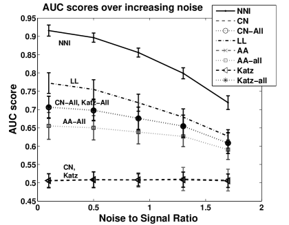
We generated -node graphs over timesteps using seasons, and plotted AUC averaged over random runs for several noise-to-signal ratios (Fig. 2). NNI consistently outperformed all other baselines by a large margin. Clearly, seasonal graphs have nonlinear linkage patterns: the best predictor of links at time are the links at times , , etc., and NNI is able to learn this pattern. By contrast, CN, AA, and Katz are biased towards predicting links between pairs which are linked (or have short paths connecting them) at the previous timestep ; this implicit smoothness assumption makes them perform poorly; indeed, they behaved essentially as poorly as a random predictor (an AUC of 0.5).
Baselines LL, CN-all, AA-all and Katz-all use information from the union of all graphs until time . Since the off-seasonal noise edges are not sufficiently large to form communities, most of the new edges come from communities of nodes created in season. This is why CN-all, AA-all and Katz-all outperform their “last-timestep” counterparts. As for LL, since links are more likely to come from the last seasons, it performed well, although poorly compared to NNI. Also note that the changing user features forces the community structures to change slowly over time; in our experiments, CN-all performed worse than it would were there was no change in the user features, since the communities stayed the same.
Table 2 summarizes the average AUC scores for graphs with seasonality, and also presents results for stationary data. In both cases, the noise was set to the smallest value in Fig. 2. For the stationary data, links formed in the last few timesteps of the training data are good predictors of future links, and so LL, CN, AA and Katz all performed very well. Interestingly, CN-all, AA-all and Katz-all were worse than their “last time-step” variants, presumably owing to the slow movement of the user features. As for NNI, it performed slightly better than all other methods for the stationary data, in addition to showing substantial improvements over the other methods for the seasonal networks.
| Seasonal | Stationary | |
|---|---|---|
| NNI | ||
| LL | ||
| CN | ||
| AA | ||
| Katz | ||
| CN-all | ||
| AA-all | ||
| Katz-all |
4.3 Real-world graphs
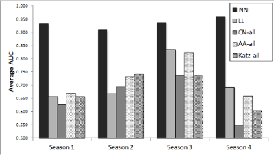
We begin by presenting results on a -node sensor network where each edge represents the successful transmission of a message222http://www.select.cs.cmu.edu/data. We considered up to consecutive measurements. These networks exhibit clear periodicity; in particular, a different set of sensors turn on and communicate during four different periods. Fig. 4 shows our results for these four periods averaged over several cycles. The maximum standard deviation, averaged over the periods, was . We do not show results for CN, AA and Katz, as they all performed no better than a random predictor. NNI significantly outperformed the baselines, confirming the results from the simulation experiments for seasonal graphs.
We also present results on three dynamic co-authorship graphs: the Physics “HepTh” community ( nodes, total edges, and timesteps), NIPS (, , ), and authors of papers on Citeseer (, , ) with “machine learning” in their abstracts. Each timestep considers years of papers (so that the median degree at any timestep is at least ). Finally we also considered a dynamic undirected network of Facebook employees over several weeks, where the nodes represent employees and edges are formed if one employee mentions another in a post. The network contains above five thousand nodes, and above edges in total.
| NIPS | HepTh | Citeseer | ||
| NNI | ||||
| LL | ||||
| CN | ||||
| AA | ||||
| Katz | ||||
| CN-all | ||||
| AA-all | ||||
| Katz-all |
Table 4 shows the average AUC for all algorithms for the co-authorship graphs and the Facebook graph. For the co-authorship graphs, we do not expect to see seasonal variation, and we expect a relatively simple model to be effective; authors will tend to keep working with a similar set of co-authors over time. For such graphs, Tylenda et al. [30] have shown that LL is the best heuristic, and we replicate that result here. Our kernel-based approach, NNI, also performs well on these graphs, slightly outperforming LL. For the Facebook graph, employees in the same research group tend to post more messages mentioning each other, and hence algorithms working on all edges seen so far should intuitively pick up this community structure. This is indeed reflected in the AUC scores. CN-all, AA-all and Katz-all perform the best. These algorithms outperform NNI, primarily because they count paths through edges that exist in different timesteps, which is not allowed in our model.
In summary, for graphs having a seasonal trend, NNI is the best method by a large margin. For the co-authorship graphs, NNI remains the best algorithm, although LL is also effective. For the correlation graph, Katz-all is the best algorithm, but its performance is quite poor on the co-authorship graphs and the seasonal graphs. Overall, the performance of NNI dominates that of the other algorithms.
4.4 Evaluation of LSH
We have found the use of LSH to be essential in our experimental work. In this section we provide quantitative support for this assertion.
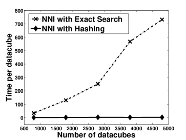
Exact search vs. LSH. In Fig. 5(a) we plot the time taken to perform top- nearest neighbor search for a query datacube using simulated data. We fixed the number of nodes at , and increased the number of timesteps. As expected, the exact search time increases linearly with the total number of datacubes, whereas LSH searches in nearly constant time. Also, the AUC score of NNI with LSH is within 0.4% of that of the exact algorithm on average, implying minimal loss of accuracy from LSH.
In our experiments with real-world graphs, the query time per datacube using LSH was quite small: s for Citeseer, s for NIPS, s for HepTh, and s for Facebook. Exact search was infeasible for these large-scale graphs.
 |
 |
| (a) Time vs. #-datacubes | (b) AUC vs. hash bitsize |
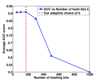
Number of Bits in Hashing. Fig. 5(b) shows the effectiveness of our adaptive scheme to select the number of hash bits (Section 3). For these experiments, we turned off the smoothing based on the prior datacube. As increases, the accuracy goes down to , as a result of the fact that NNI fails to find any matches of the query datacube. Our adaptive scheme finds , which yields the highest accuracy. Note also that larger translates to fewer entries per hash bucket and hence faster searches, and thus our adaptive choice of yields the fastest runtime performance as well.
5 Consistency of Kernel Estimator
In this section we study the consistency of the estimator defined in Eq. (3). Recall that our model is:
| (5) |
where equals . Assume that all graphs have nodes ( is finite). For a fixed node , let represent the query datacube . We want to study the consistency of predictions for timestep .
Rather than studying directly, it proves to be simpler to study a slightly different estimator which we show (in Lemma 5.1) to be asymptotically equivalent to . Define and as follows:
| (6) | ||||
Proof.
Recall that denotes the set of features at distance from . Let . We have:
where by virtue of the finiteness of number of features, and , we have:
Similarly, . Also, note that both and are non-negative. Thus we have:
where the last step follows because both and are bounded and tends to some positive constant with probability tending to one as (as shown in Theorem 5.2). ∎
The estimator is defined only when , which holds with probability tending to one as will be shown in the next theorem. The kernel was defined earlier as , where the bandwidth tends to as , and is the distance function defined in Eq. (4). This has the following property:
| (7) |
From now on, we will drop the arguments and and instead write , , and for simplicity. Our graph evolution model is Markovian; assuming each “state” to represent consecutive graphs, the next graph (and hence the next state) is a function only of the current state. The state space is also finite, since each graph has bounded size. Thus, the state space may be partitioned into a set of transient states and , where is an irreducible closed communication class, and there exists at least one [7].
The Markov chain must eventually enter one of the (finitely many) communication classes. We will denote the time of entering some communication class by , and the event by . We remind the reader that using simple arguments for finite state space Markov chains, it can be shown that the tail probability of decays geometrically (see [7]), leading to the finiteness of the first and second moments. Also let denote the event , where denotes the state of the Markov chain at time . Thus is the event that the chain enters class at time and remains there henceforth.
Theorem 5.2 (Consistency).
Let as . For two fixed nodes , is well-defined with probability tending to one as . Also, is a consistent estimator of , i.e., as .
Proof.
First, note that our query datacube is obtained at time , and we are interested in the asymptotic behavior of the chain as . Since our Markov chain has a finite state space, the query datacube belongs to some closed communication class with probability tending to one. Thus, as , the estimator’s distribution is governed by that communication class. We prove our result in two parts; first we show that the convergence statement holds conditioned on , for any communication class ; i.e., as . Next, we have
which implies , given the tail bound on and the fact that the first term is a sum over a finite number of terms, each converging to zero as . In what follows, we will give a proof of statistical consistency conditioned on for any communication class .
Define . We have:
| (8) |
Lemma 5.3 shows that , being a positive deterministic function of class . Thus, is asymptotically well defined. Also Lemma 5.9 shows that tends to as . This along with Lemma 5.3 shows that, conditioned on , , thus also proving that is asymptotically well defined for .
Next, we will define the following:
| (9) |
Note that and (Equation 6) equals and respectively. Also let
| (10) |
Thus is a bounded deterministic function of the state at time . In Lemma 5.9 we prove that for some non-negative constant , as . Thus we have, , as . Since , we have conditioned on .
Since convergence in quadratic mean implies convergence in probability, we have:
Using the continuous mapping theorem on and the fact that (Lemma 5.4) we have that, for any such that , . ∎
The proof of the following lemma is deferred to the Appendix.
Lemma 5.3.
As , for some (a deterministic function of class ),
| , |
The following smoothness condition on is introduced to ensure appropriate rates of convergence of the bias terms .
Assumption 1.
The function satisfies the following smoothness condition with respect to the distance metric : .
Lemma 5.4.
Define . If Assumption 1 holds, then we have . Since as , this implies .
Proof Sketch.
For , and , the numerator of is an average of the terms:
Using a further conditioning step on , we can show that the numerator of can be upper bounded as:
We now analyze each term in the average; i.e., terms of the form:
This expectation is computed over all possible configurations of the neighborhoods and . Since our neighborhood sizes are bounded (because is bounded), the expectation is a sum over a finite number of terms.
We now use the smoothness assumption on . Using and that is finite for all and Lemma 5.3, we have:
which holds because for non-negative , we have . ∎
We now show that the variance of and converge to zero. In order to upper bound the growth of variance terms, we make use of strong mixing. For a Markov chain , define the strong mixing coefficients , where and are the sigma algebras generated by events in and respectively. Intuitively, small values of imply that states that are apart in the Markov chain are almost independent. For bounded and , this also limits their covariance: for some constant [5]. Instead of proving that the variance of or converges to zero, we will prove that the variance divided by converges to a non-negative constant. This is a stronger result that we will find useful in proving weak convergence in section 7.
We introduce some notation that will be used in stating the next few results. Let denote a bounded deterministic function of the state of a finite state space Markov chain at time . Also define . Recall that our Markov chain will eventually hit one of the finitely many closed communication classes. Earlier we used to define the event , by the time of entering some communication class, and the event by . We will denote the event of entering class at time by . If is aperiodic, then once inside , the Markov chain gets arbitrarily close to the stationary distribution of after some constant time ; we state this more formally in the following lemma, whose proof is deferred to the Appendix.
Lemma 5.5.
Consider an irreducible and aperiodic finite state Markov chain with probability transition matrix , initial distribution and stationary distribution . Let be a random variable (with finite support) that is conditionally independent of all other states, given the state at time . The expectation of under the distribution at time is denoted by . Let denote the expectation of (i.e., the expectation with respect to ). There exists a constant , and a constant such that, for all , , and .
Our estimators are weighted sums of variables; for , we will break this sum up into three parts, indexed by , followed by , and finally , where is a constant. For , we will use the fact that has bounded first and second moments. Since we are interested in the behavior of the sum unconditionally, our analysis will consist of two steps of nested conditioning, the outer one obtained by conditioning on , which in turn is obtained by analyzing the sum conditioned on . For ease of exposition we will assume to be aperiodic. The more general case of cyclo-stationarity, which is similar in principle, is discussed in remark 5.10.
Lemma 5.6.
as , for some constant .
Proof.
Lemma 5.7.
For any finite integer , we have
| (11) | ||||
| (12) |
For a Markov chain with a finite state space, we also have for some .
Proof Sketch.
For ease of exposition, for the proof sketch we assume there is only one communication class, which is aperiodic. Recall that is the time to hit the communication class. Once inside the communication class, irreducibility and aperiodicity implies geometric ergodicity (Lemma 5.5), which implies absolute regularity which in turn implies strong mixing with exponential decay [3]: for some . We can prove that for finite , . So we focus on proving Equation 11. Denote by .
Recall that for our Markov chain, involves graphs (). Since is a function of , it also depends on graphs. Hence, the distance between two sigma-algebras and is defined as . Now we can write as
Since the number of states at distance is , and at distance is , for constants we have,
This shows that the above sum converges to some constant . Since , the chain will get arbitrarily close to stationarity, and for some constant . Thus is asymptotically equivalent to , which also converges to as . Since, for all , is non-negative, is also non-negative. This proves Equation 11. Thus Equation 12 is proved, and also, since has finite first and second moments for a finite state space Markov chain, converges to , as . ∎
It remains to analyze in the variance decomposition. Using Lemma 5.5 we can prove that approaches zero at a geometric rate as , where denotes the expectation of under the stationary distribution in communication class . This implies the following lemma, which is proved in the Appendix.
Lemma 5.8.
.
Lemma 5.9.
and tend to as .
Proof.
The result follows by applying Lemma 5.6 with equal to
and
respectively.
∎
Remark 5.10.
Recall that Lemma 5.7 was obtained under the assumption that is aperiodic. The case of periodic implies cyclo-stationarity; i.e., the chain approaches stationarity as . Hence, for periodic (with period ) we consider , which is a Markov chain where each transition corresponds to transitions of the original chain. Now, is irreducible and aperiodic (since was irreducible and had period ). A state in started at simply corresponds to the old state in . Now, can be written as , where is the sum of consecutive random variables. Since, is independent of all other s conditioned on , we have:
| (13) | |||
The last step uses the fact that the are bounded. Now, can again be shown to converge to some non-negative constant using a slight modification of the argument in Lemma 5.7. The remainder of can be shown to be negligible via a simple application of the Cauchy-Schwartz inequality. A detailed proof of Lemma 5.7 using this idea can be found in the Appendix.
As for in the cyclic case, we simply have to apply Lemma 5.5 for each of the cyclic classes. For the cyclic class, is independent of all states (in that cyclic class) given . Hence there exists , and , such that for all with , , thus proving Lemma 5.5 for a periodic . This again proves Lemma 5.8 for the case where is periodic.
6 Stein’s Method for Graphical Data
Our estimators, and indeed many kernel estimators, involve weighted sums of dependent variables. While their distributional convergence can be studied using existing results on ergodic Markov chains, we take a different approach, based on an adaptation of Stein’s method to the setting of graphs.
We begin with a brief introduction to Stein’s method. The method reposes on the following key lemma [4], which provides a characterization of the normal distribution:
Lemma 6.1 (Stein’s Lemma).
If has a standard normal distribution, then
| (14) |
for all absolutely continuous functions with . Conversely, if Equation 14 holds for all bounded, continuous and piecewise continuously differentiable functions with , then has a standard normal distribution.
Recall that the Wasserstein distance between a mean zero, unit variance random variable and a standard normal variate is defined as , where . Weak convergence of to can be established by showing that the Wasserstein distance converges to zero. Now, Stein’s Lemma (6.1) shows that if equals zero for appropriate choices of . This key observation leads to the Stein Equation:
| (15) |
It can be shown that the solution to the Stein Equation, for , satisfies , , [4]. Thus, instead of dealing with we need to show that is small (where satisfies the aforementioned conditions); this is an easier quantity to analyze.
The existing application of Stein’s method to sums of weakly dependent random variables has focused on marginal-independence structures that can be captured by a bounded-degree dependency graph [25]. In this section, we relax the requirement of marginal independence by allowing arbitrary dependency structures among the summed variables as long as certain conditions on strong mixing coefficients hold. (See also Sunklodas [28] for a similar approach to ours for chain-structured dependencies; he obtains a slightly tighter bound than ours at the expense of a more complex proof.)
Our approach proceeds by bounding the Wasserstein distance between the (appropriately scaled and centered) sum of the dependent variables and a standard normal variate in terms of and the degree of dependence of the random variables. We then show that this bound tends to zero for our estimators, demonstrating convergence to a normal distribution and yielding a rate of convergence as a by-product. We note that although we use this to prove normal convergence for a cyclo-stationary Markov chain, it can potentially be used for more general dependence structures, as long as suitable strong mixing properties are available.
We let denote the total number of variables in our model. Let be bounded, (), mean-zero random variables. Let denote the variance of ; assume for all . Define , where . Let , and . We will assume that the index set underlying the random variables is endowed with a distance metric, . This can be the geodesic distance if the variables are connected via a graph structure or the absolute difference in time indices in a time series model, etc. Let denote the set of nodes at distance from node ; similarly let and respectively denote the set of nodes within distance and at a distance greater than from node . Now, let denote .
We need a notion of strong mixing in a network setting. Define the strong mixing coefficients , where is the sigma algebra generated by the random variable . A similar proposal for strong mixing in random fields can be found in [21]. Let denote the tail sum . We are now ready to state the main result.
Lemma 6.2.
The Wasserstein distance between and the standard normal random variable is upper bounded as follows:
| (16) | ||||
where are constants.
Proof sketch.
We will give a brief proof sketch here, and provide the full proof in the Appendix. We want to bound . We shall repeatedly break up into two parts: being the contribution from all nodes with distance more than from some node , and the remainder from nodes “close to” . In classical analysis of dependency graphs, and are independent; in contrast, in our case we only have . Here, is a parameter that shall be picked later to optimize the bound. Since ,
Using Taylor expansion the term can be further bounded by
The first term of this result again can be bounded using the AM-GM inequality by , where is a constant. Recall that upper bounds the size of the neighborhood of hops. The second part of (A2) now is bounded by , using the usual relationship between covariances and strong mixing coefficients. Thus the overall bound on is as follows:
Now we need to bound . Denote . Note that if and were independent, we would have , since is centered and scaled appropriately. For us however does not equal ; instead it becomes smaller as we increase . We thus bound as follows:
Now note that . Since ,
using the fact that , and for all , . We upper bound by . Using similar arguments (see Appendix) we upper bound by .
Putting the pieces together and using we see that
The result is obtained by optimizing the upper bound over . ∎
Next, we present a sufficient condition for the Wasserstein distance to vanish asymptotically, implying convergence of to a standard normal.
Lemma 6.3.
as if the following conditions hold:
-
1.
.
-
2.
There exists a sequence such that the following are satisfied:
-
(a)
-
(b)
-
(c)
.
-
(a)
Proof.
The above conditions imply that , , and (and thus as well) as . Hence the product of two vanishing sequences, , also vanishes. Similarly also vanishes as . Thus, all terms on the right hand side of Eq. (16) vanish, thus proving . ∎
7 Weak Convergence of our Estimator
In this section we bring together the results from the previous two sections to establish weak convergence of our estimator.
Recall that our estimator is defined in Equation 3. Recall also the definitions of , and from Equations 9 and 10. From Lemma 5.1 we have , where denotes the bandwidth for the pair-specific kernel function (see Equation 2). Hence, with for some , we see that . We will show (in Proposition 7.1) that under suitable conditions converges to a mean-zero normal distribution. Hence, we also have the same normal distribution as the limit of under the same conditions.
Proposition 7.1.
Proof.
From Equation 8 we see that equals . Using the following lemma (Lemma 7.2) we know that the numerator of the first term converges to a distribution. Using Lemmas 5.9 and 5.3 we have for a positive constant , conditioned on . Hence using Slutsky’s lemma the first part converges conditionally to . Also, converges to one in probability conditioned on . Finally, invoking Lemma 5.3 and Lemma 5.4 we see that since , for , the second part is . Now, Slutsky’s lemma and the continuous mapping theorem yield the statement of the proposition. ∎
Lemma 7.2.
Under Assumption 1 and assuming ,
The proof of this result uses Lemma 5.8 and is deferred to the Appendix.
Lemma 7.3.
Define . Under Assumption 1 and assuming , for any finite , we have:
Proof Sketch.
First we prove that, for a sequence for a properly chosen , the conditions in Lemma 6.3 are satisfied for
We also show that for this value of , the upper bound on the Wasserstein distance in Lemma 6.2 is . The details are deferred to the Appendix. Now Lemma 6.1 gives:
However, for finite values of , (Lemma 5.7 and Equation 11). Thus, the additional assumption of proves the result. ∎
Remark 7.4.
Proposition 7.1 shows that, under some weak assumptions, converges to a standard normal distribution conditioned on . Since there are a finite number of closed communication classes, unconditionally converges to a mixture of zero-mean Gaussians, the mixture proportions being determined by the probability of reaching the communication classes from the start state.
Remark 7.5.
We have established weak convergence for the case where is aperiodic. However, as in Remark 5.10, we can consider , which is a Markov chain where each transition corresponds to transitions of the original chain. Again, any sum of the form can be written as . now denotes the sum of the consecutive ’s. For , we have using Equation 13. Thus the first sum again brings us to the irreducible aperiodic setting (with a slightly modified distance function), and hence normal convergence can be established.
8 Related Work
Existing work on link prediction in dynamic networks can be broadly divided into two categories: link prediction based on generative models and link prediction based on structural features.
A substantial amount of work has gone into the development of generative models of graph structure based on the formalism of Markov random fields, loglinear models or other graphical models [6, 8, 15, 26, 11, 29, 31]. For example, Hanneke and Xing [8] present a dynamic loglinear model based on evolution statistics such as “edge stability,” “reciprocity” and “transitivity.” Fu et al. [6] propose an extension of the mixed membership block model to allow a linear Gaussian trend in the model parameters. Zhou et al. [34] present a nonparametric approach to estimating a time-varying Gaussian graphical model where the covariance matrix changes smoothly over time. The discrete analog of this is considered in [15], where the goal is to learn the latent structures of evolving graphs from a time series of node attributes. The static model of Raftery et al. [23] is extended by Sarkar and Moore [26] by allowing smooth transitions in latent space. All of these models have the virtue of a clean probabilistic formulation such that link prediction can be cast in terms of Bayesian posterior inference. Obtaining this posterior is, however, often infeasible in large-scale graphs. Moreover, these models often make strong model assumptions, not only for the graph structure but also for the network dynamics, which is often modeled as linear.
Alternatives to generative models generally revolve around the definition of various static features that aim to capture structural properties of graphs. These are extended to the dynamic setting via heuristics or via autoregressive modeling. For example, Huang and Lin [12] propose a linear autoregressive model for link prediction and investigate simple combinations of static graph-based similarity measures (e.g., Katz, common neighbors) with their autoregressive model to capture transitive similarities in networks. A similar parametric approach can be found in Richard et al. [24], where a vector autoregressive model was used for link prediction in dynamic graphs. The authors assume a low rank structure of the graph adjacency matrices and propose proximal methods for inference.
Tylenda et al. [30] examine simple temporal extensions of existing static measures. As we have noted earlier, these methods have the virtue of being applicable to large-scale graphs. They also tend to yield surprisingly good performance. Our work falls into this general category, while going beyond existing work by providing a formal statistical treatment of link prediction as a nonparametric estimation problem.
We conclude this section with a brief discussion on relevant research on nonparametric bootstrap estimators in strong mixing random fields and Markov processes. While these works are not relevant to the link prediction aspect of our work, they are similar because the estimation uses local resampling methods thereby retaining the dependency structure of the data. In the context of strong mixing random fields Politis and Romano [22] consider a blocks of blocks re-sampling method for estimating asymptotically accurate confidence intervals for parameters of the joint distribution of the random field. Nonparametric bootstrap algorithms have also been applied successfully to the area of computer vision. Levina and Bickel [16] show that one such heuristic algorithm for texture synthesis can be formally framed as a resampling technique for stationary random fields, and prove consistency properties of it under broad conditions. In the context of stochastic processes with an autoregressive structure, Paparoditis and Politis [19] present the “local bootstrap” algorithm, which implicitly estimates the distribution of the one-step transition in the underlying Markov process and generates the bootstrap replicates using this estimated distribution.
9 Conclusions
In this paper we proposed a nonparametric model (NNI) for link prediction in dynamic networks, and showed that it performs as well as the state of the art for several real-world graphs, and exhibits important advantages over them in the presence of nonlinearities such as seasonality patterns. NNI also allows us to incorporate features external to graph topology into the link prediction algorithm, and its asymptotic convergence to the true link probability is guaranteed under our fairly general model assumptions. In addition, we show how to make NNI computationally tractable via the use of locality sensitive hashing. Together, these make NNI a useful tool for link prediction in dynamic networks.
10 Appendix
10.1 Statement and proofs of results from section 5
Lemma 5.3.
As , for some (a deterministic function of class ),
| , |
Proof.
Let denote the minimum distance between two datacubes that are not identical; since the set of all possible datacubes is finite, . is an average of terms , over and . Now,
Writing the expectation in terms of a sum over all possible datacubes, and noting that everything is bounded, gives the following:
Recalling that was an average of the above terms, we see that it equals:
| (17) |
We will now show that the above average converges to for some . The second term in the RHS in eq (17) converges to zero, since as . For the numerator of the first term we have, . Both and are fully determined given the current state of the Markov chain. Using to denote an indicator of in state , we have . As a result of this, the first term in the R.H.S of eq (17) becomes an average of the form , where . Since we have a finite state-space and is bounded, we can rewrite the above expression as .
Now, recall that the query datacube at is a function of the state , which belongs to a closed irreducible set with probability . Due to stationarity (or cyclic stationarity with a finite cycle length) the average converges to some constant (constant because it is a function of the finite state space). For the special case of , we have the following: (a) , so , and (b) contains at least one pair of nodes with the feature vector (since we are attempting link prediction for such a pair), so there exists some for which . Together, these imply that converges to some , where is a deterministic function of communication class .
Noting that , and the fact that is bounded we invoke the Dominated Convergence Theorem and see that as well, thus completing the proof of the theorem.
∎
Lemma 5.4.
Define . If assumption 1 holds, then, we have . Since as , this implies .
Proof.
For , the numerator of is an average of the terms:
Taking expectations w.r.t. , and denoting by , the first term becomes:
Now note that . Conditioning on makes conditionally independent of given if . Also, for , , as can be seen by summing Eq. 2.3 over all pairs in a neighborhood with identical , and then taking expectations333Note that the conditioning on is crucial here.. This along with the fact that is bounded leads to:
Thus the numerator of can be upper bounded as:
The second part is simply and . Thus, the numerator of becomes an average of the terms of the following form:
This expectation is over all possible configurations of the neighborhoods and . Since our neighborhood sizes are bounded (because is bounded), the expectation is a sum over a finite number of terms.
We now use the smoothness assumption on . Using and that is finite for all and Lemma 5.3, we have:
The last equation holds since for non-negative , . ∎
Lemma 5.5.
Consider an irreducible and aperiodic finite state Markov chain with probability transition matrix , starting distribution and stationary distribution . Let be a deterministic function (with finite support) of the state at time . The expectation of under the distribution at time is denoted by . Let denote the expectation of (i.e. under distribution ). There exists a constant , and a constant such that, , , and .
Proof.
Using the same line of reasoning as [9], we first prove the above for . Here denotes the state space and the probability transition matrix associated with the Markov chain. Denote by the matrix , where denotes the column vector of all ones. Note that since and , we have . For a finite state space irreducible and aperiodic Markov chain, , as . Hence for some positive , we can find an s.t. , , . Since , using matrix norm inequalities we have for , where and ,
since is a constant. However, , where . Now for and , we have:
First consider to be an atom at a state . Since , using that is bounded we have the main result. The result can be easily extended to the more general case where is a convex combination of atoms at . ∎
Lemma 5.7.
For any finite integer , we have
| (7) | ||||
| (8) |
For a finite state space Markov chain, we also have for some .
Proof.
Let have (finite) period ; the period is finite from the finiteness of the Markov chain, and is typically very small (e.g., if everywhere). Let be a Markov chain where each transition corresponds to transitions of the original chain. Now, is irreducible and aperiodic (since was irreducible and had period ). Thus, s.t. , it is geometrically ergodic with rate (Lemma 5.5), which implies in turn that for , is strongly mixing with exponential drop-off [20] for large : for some . Thus, distant states are almost independent, and we use this to bound the covariances of the , as follows. Also define .
For the first term, we have:
First, note that . We now focus on . Let , and . Thus,
, as for , we have:
Recall that for our Markov chain, involves graphs (). Since is a function of , it also depends on graphs. Hence, the distance between two sigma-algebras and is defined as . Thus, the total number of states at distance is . Let Rather importantly, note that we will use basic conditional independence results from Markov chains. For example . Unfortunately, conditioned on this may not be true. However, if , we can safely use the conditional independence, which is definitely true for .
For notational convenience we will denote by and covariance and expectation conditioned on . Then,
| (letting and ) | |||
Recall that we were originally interested in . Let us first consider . By virtue of geometric ergodicity , where . Thus we have:
Using elementary arguments from real analysis we see that converges to some finite number. Hence after dividing by it contributes a term to the expression . For this reason we will now concentrate on term. First note that the sequence is upper bounded by the following,
We again see that also converges to some constant , thus making asymptotically equivalent to: . However, for all , if the chain is cyclo-stationary, then after a finite time, for any , approaches the same constant , . Therefore, for all we have , where is a constant w.r.t . This leads to:
Since the is a variance term, it is non-negative for all , and hence must be non-negative as well, thus proving Equation 7. Using the Cauchy Schwartz inequality,
Thus as for some non-negative constant .
Another use of the Cauchy Schwartz argument from before, along with the convergence result on lets us upper bound by .
Thus, for finite , putting all the bounds (i.e. on , , and ) together, we have , for some , proving Equation 8. Also, since has finite first and second moments for a finite space Markov chain, we have .
We remind the reader that using simple arguments for finite state space Markov chains, it can be shown that ’s tail probability is geometrically decaying, leading to the finiteness of the first and second moments.
∎
Lemma 5.8.
.
Proof.
Recall that . Let denotes the expectation of under the stationary distribution in communication class (it is a deterministic function of class ). Since , we will simply upper bound . Lemma 5.5 shows that: , and such that, , . Thus,
| (9) |
Thus, , since has finite second moment. ∎
10.2 Statement and proofs of results from section 6
Lemma 6.2.
The Wasserstein distance between and the standard normal random variable is upper bounded as follows:
where are constants.
Proof.
We define the following sets:
We also define the following upper bounds on the sizes of these sets:
Before beginning, we recall two facts.
(1) Bounded covariance via strong mixing: For two random variables and that are more than distance away, we have
(2) Bounds on Wasserstein distance: For the set of functions ,
where is the Wasserstein distance and has the standard normal distribution.
In the following, we shall bound . We shall repeatedly break up into two parts: being the contribution from all nodes within a distance of some node , and the remainder from nodes “far away” from . Here, is a parameter that shall be picked later. We can bound as follows:
| (10) | |||
The second part in eq. 10 can be further bounded above as follows,
| (11) | |||
where the second inequality follows from Taylor expansion with being some value between and .
First, note that:
As for the second term in eq. 11 we have:
Thus, we obtain a bound for both terms in eq. 11, and hence a bound for the second term of eq. 10. We will now bound the first term in eq. 10. Let . Denote by the tail sum . Recall that and . Thus,
Now,
Next, we look at the term:
| (12) | ||||
The first term (i.e., term (A)) in eq. 12 can be broken into two parts, one such that the minimum distance between any node in and any node in pair is (denote this by set ), and one where its greater than (denote this by set ). Formally, we define the following terms:
Consider the term . Given , can be picked in at most ways. Now, either or or both must be within distance of or . Thus, given and , (or ) can be picked in at most ways, and then (or ) can be picked in another ways. Hence, . By a similar argument,
Now, we have:
10.3 Statement and proofs of results from section 7
We will start by reminding the reader some of the definitions. Define the following:
We define: , and . Also, .
Lemma 7.2.
Under Assumption 1 and assuming ,
Proof.
Using our distributional convergence results conditioned on , we have shown that
Denote by . We have,
| (13) | |||
where , and are positive constants. Let denote the c.d.f of , i.e. . Lemma 7.4 tells us that, for finite and , ; being the c.d.f of a normal distribution with mean zero, and standard deviation . Now, using Equation 13 we have the following simple argument:
In the last step, the exchange of limit and expectation is valid by virtue of the Dominated Convergence Theorem. Now taking (which minimizes the upper bound on the ) and using the geometric bound on tail probability of in finite state space Markov chains, we have:
An identical argument on gives the following equation.
Thus we show that , which in turn proves our result. ∎
Lemma 7.3.
Define . Under Assumption 1 and assuming , for any finite , we have:
Proof.
We will prove the above result in two parts. If we can show that the conditions in Lemma 6.3 are satisfied for
then using Lemma 6.1 we will have:
However, for any finite value of , (see Lemma 5.7, eq. 7). Thus, with the additional assumption of , the result is proved.
Now we will show that, conditioned on , the conditions in Lemma 6.3 are satisfied for , and thus the Wasserstein distance in Lemma 6.2 can be upper bounded by .
First note that is bounded and . Thus corresponds to in Lemma 6.2. Since is a function of , it involves graphs (). The distance is defined as . Thus equals for , and otherwise; hence . Also, . Denote by the standard deviation of conditioned on . Let us now examine the conditions in Lemma 6.3.
Condition 1
We have , where the limits follow from Lemma 5.7 and the assumption.
Condition 2
Let . We will show that this satisfies conditions 2a, 2b, and 2c.
2a:
-
Plugging in the value of , and using Lemma 5.7 we see that:
2b:
-
Using Lemma 5.7 we see that:
2c:
-
Again, using Lemma 5.7 gives us:
Now the upper bound on Wasserstein distance (Lemma 6.2) becomes by using and the expressions derived before as part of the second condition. ∎
Acknowledgements
We are grateful to Peter Bickel for helpful discussions on this topic.
References
- Adamic and Adar [2003] L. Adamic and E. Adar. Friends and neighbors on the web. Social Networks, 25:211–230, 2003.
- Aitchison and Aitken [1976] J. Aitchison and C. G. G. Aitken. Multivariate binary discrimination by the kernel method. Biometrika, 63:413–420, 1976.
- Bradley [2005] R. C. Bradley. Basic Properties of Strong Mixing Conditions. A Survey and Some Open Questions. Probability Surveys, 2:107–144, 2005.
- Chen et al. [2010] L.H.Y. Chen, L. Goldstein, and Q.M. Shao. Normal Approximation by Stein’s Method. Springer Verlag, 2010.
- Durrett [1995] R. Durrett. Probability: Theory and Examples. Duxbury Press, 1995.
- Fu et al. [2010] W. Fu, E. P. Xing, and L. Song. A state-space mixed membership blockmodel for dynamic network tomography. Annals of Applied Statistics, 4:535–566, 2010.
- Grimmett and Stirzaker [2001] G. Grimmett and D. Stirzaker. Probability and Random Processes. Oxford University Press, 2001.
- Hanneke and Xing [2006] S. Hanneke and E. P. Xing. Discrete temporal models of social networks. Electronic Journal of Statistics, 4:585–605, 2006.
- Heidergott et al. [2005] B. Heidergott, A. Hordijk, and M. van Uitert. Series expansions for finite-state Markov chains. Tinbergen Institute Discussion Papers 05-086/4, 2005.
- [10] P. D. Hoff. Latent factor models for relational data. URL http://www.stat.washington.edu/hoff/public/acms.pdf.
- Holland and Leinhardt [1977] P. W. Holland and S. Leinhardt. A dynamic model for social networks. Journal of Mathematical Sociology, 5:5–20, 1977.
- Huang and Lin [2009] Z. Huang and D. K. J. Lin. The time-series link prediction problem with applications in communication surveillance. INFORMS Journal on Computing, 2009.
- Indyk and Motwani [1998] P. Indyk and R. Motwani. Approximate nearest neighbors: Towards removing the curse of dimensionality. In ACM Symposium on Theory of computing. MIT Press, 1998.
- Katz [1953] L. Katz. A new status index derived from sociometric analysis. In Psychometrika, volume 18, pages 39–43, 1953.
- Kolar et al. [2010] M. Kolar, L. Song, A. Ahmed, and E. Xing. Estimating time-varying networks. Annals of Applied Statistics, 2010.
- Levina and Bickel [2006] Elizaveta Levina and Peter J. Bickel. Thexture synthesis and nonparametric resampling of random fields. Annals of Statistics, 34(4):1751 1773, 2006.
- Liben-Nowell and Kleinberg [2003] D. Liben-Nowell and J. Kleinberg. The link prediction problem for social networks. In Conference on Information and Knowledge Management. ACM, 2003.
- Masry and Tjøstheim [1995] E. Masry and D. Tjøstheim. Nonparametric estimation and identification of nonlinear ARCH time series. Econometric Theory, 11:258–289, 1995.
- Paparoditis and Politis [2002] Efstathios Paparoditis and Dimitris N. Politis. The local bootstrap for markov processes. J. Statist. Plann. Inference, 108:301–328, 2002.
- Pham [1986] D. Pham. The mixing property of bilinear and generalised random coefficient autoregressive models. Stochastic Processes and their Applications, 23:291–300, 1986.
- Politis et al. [1999] D. Politis, J. Romano, and M. Wolf. Subsampling. Springer, 1999.
- Politis and Romano [1993] D. N. Politis and J. P. Romano. Nonparametric resampling for homogeneous strong mixing random fields. Journal of Multivariate Analysis, 47(2):301–328, 1993.
- Raftery et al. [2002] A. E. Raftery, M. S. Handcock, and P. D. Hoff. Latent space approaches to social network analysis. Journal of the American Statistical Association, 15:460, 2002.
- Richard et al. [2012] Emile Richard, Stephane Gaiffas, and Nicolas Vayatis. Link prediction in graphs with autoregressive features. In P. Bartlett, F.C.N. Pereira, C.J.C. Burges, L. Bottou, and K.Q. Weinberger, editors, Advances in Neural Information Processing Systems 25, pages 2843–2851, 2012.
- Rinott and Rotar [1996] Y. Rinott and V. Rotar. A multivariate CLT for local dependence with rate and applications to multivariate graph related statistics. Journal of Multivariate Analysis, 56(2):333–350, 1996.
- Sarkar and Moore [2005] P. Sarkar and A. Moore. Dynamic social network analysis using latent space models. In Advances in Neural Information Processing Systems. 2005.
- Sarkar et al. [2008] P. Sarkar, L. Chen, and A. Dubrawski. Dynamic network model for predicting occurrences of salmonella at food facilities. In Biosurveillance and Biosecurity: International Workshop, BioSecure. Springer, 2008.
- Sunklodas [2007] J. Sunklodas. On normal approximation for strongly mixing random variables. Acta Applicandae Mathematicae, 97:251–260, 2007.
- T Snijders [1997] K Nowicki T Snijders. Estimation and prediction for stochastic blockmodels for graphs with latent block structure. Journal of Classification, 1997.
- Tylenda et al. [2009] T. Tylenda, R. Angelova, and S. Bedathur. Towards time-aware link prediction in evolving social networks. In ACM Workshop on Social Network Mining and Analysis. ACM, 2009.
- Vu et al. [2011] D. Vu, A. Asuncion, D. Hunter, and P. Smyth. Continuous-time regression models for longitudinal networks. In Advances in Neural Information Processing Systems. MIT Press, 2011.
- Wang and van Ryzin [1981] M.-C. Wang and J. van Ryzin. A class of smooth estimators for discrete distributions. Biometrika, 1981.
- Wilson [1927] E. Wilson. Probable inference, the law of succession, and statistical inference. Journal of the American Statistical Association, 22:209–212, 1927.
- Zhou et al. [2008] S. Zhou, J. Lafferty, and L. Wasserman. Time varying undirected graphs. In Conference on Learning Theory, 2008.