Soliton Creation with a Twist

Abstract

We consider soliton creation when there are “twist” degrees of freedom present in the model in addition to those that make up the soliton. Specifically we consider a deformed O(3) sigma model in 1+1 dimensions, which reduces to the sine-Gordon model in the zero twist sector. We study the scattering of two or more breather solutions as a function of twist, and find soliton creation for a range of parameters. We speculate on the application of these ideas, in particular on the possible role of magnetic helicity, to the production of magnetic monopoles, and the violation of baryon number in nuclear scattering experiments.

Field theories are known to have two sectors – small excitations called “particles”, and large excitations called “solitons”. Perturbative quantum field theory deals with particles and their interactions. Solitons are generally studied as classical solutions, unrelated to the particle description. An outstanding open problem in quantum field theory is to describe solitons as an assembly of particles. A closely related problem is the central focus of this paper – how can we build solitons by scattering particles?

The relation between solitons and particles is explicitly known in the sine-Gordon model Mandelstam:1975hb where the soliton operator is given in terms of an infinite number of particle operators. Thus to build solitons from particles in the sine-Gordon model requires assembly of an infinite number of particles and is impossible. This ties in with the complete integrability of the sine-Gordon model wherein soliton number is preserved. Therefore it is necessary to consider models that are not completely integrable. However integrable models are amenable to a lot of analysis, and it seems unwise to abandon them altogether. We would like to take advantage of the insights that are provided by integrable models and to use them in a non-integrable setting. Hence we aim to start with a completely integrable model, modify it suitably to eliminate complete integrability while still preserving as many features as possible, and then study soliton creation in the non-integrable model.

There can of course be many modifications of a completely integrable model. Indeed, the $\lambda\phi^{4}$ model in 1+1 dimensions studied in Dutta:2008jt ; Romanczukiewicz:2010eg ; Demidov:2011eu can also be viewed as a deformation of the sine-Gordon model. Here we would like to study a different kind of modification; one that may be useful in generalization to higher spatial dimensions where we would like to study the creation of vortices and magnetic monopoles. The modification is inspired by recent work within the electroweak model Copi:2008he ; Chu:2011tx : the annihilation of “twisted” magnetic monopoles leads to the production of magnetic fields that inherit the twist in the form of magnetic helicity. We will describe this observation in greater detail in Sec. IV. For the time being we note that magnetic monopoles can carry a relative twist, and so we would like to introduce a similar twist degree of freedom in the 1+1 dimensional sine-Gordon model, thus also breaking complete integrability. Then the kinks of the sine-Gordon model will be able to carry relative twist, and solitons may be created in scattering that involves the twist degree of freedom. The hope is that twisted initial conditions are better suited to the creation of solitons. In our toy model in Sec. I we will see that twist is essential for the creation of solitons because untwisted initial conditions lie in a completely integrable sub-space of the model.

A different view of the soliton creation problem also suggests that twist can play a useful role. When two particles scatter, it is advantageous if they spend a long time together, so that other particles also have time to interact and create a multi-particle state such as the soliton-antisoliton pair. In our case, we will take the initial state to be a sequence of sine-Gordon breathers – the closest we can come to a sequence of particles in classical theory. When two in-phase breathers scatter in the sine-Gordon model, they pass through each other but with a negative time delay i.e. a time advance. This is because of an attractive force between the breathers. If the breathers are twisted, however, the force can be repulsive, and the scattering can lead to a time delay. In Sec. II we will study the scattering of two breathers as a function of twist. The numerical results confirm that twist can lead to a positive time delay in the scattering

The paper is organized as follows. In Sec. I we describe our toy model, and various solutions in it. In Sec. II we study the scattering of two breather solutions of the model and show that twisted breathers lead to a time delay in the scattering. As a special case we find the time delay in the scattering of two sine-Gordon breathers. In Sec. III we study the scattering of two sequences (“trains”) of twisted breathers by numerically evolving the equations of motion. Here we find examples of soliton creation. We discuss generalizations to higher spacetime dimensions, and to vortices and monopoles in Sec. IV. The production of magnetic monopoles is intimately related to baryon number violation via electroweak sphaleron production. We discuss this connection in Sec. IV, where we also conclude. In Appendix A we provide some notes related to the numerical evolution of the constrained O(3) system.

I Deformed O(3) model

With the motivation described above, we now move on to describe a model in 1+1 dimensions that contains kinks and also allows for twist. We start with the O(3) sigma model given by the action

$$S_{\sigma}=\int d^{2}x\frac{1}{2}(\partial_{\mu}{\hat{n}})^{2}$$ (1)

where ${\hat{n}}={\hat{n}}(t,x)$ satisfies the constraint

$${\hat{n}}^{2}=1$$ (2)

This model is known to be completely integrable Zamolodchikov:1978xm and we will need to spoil this feature. So we consider

$$S=\int d^{2}x\left[\frac{1}{2}(\partial_{\mu}{\hat{n}})^{2}-\frac{1}{2}(1-n_{3}^{2})\right]$$ (3)

where $n_{3}$ is the third (or $z-$) component of ${\hat{n}}$. The additional potential term spoils the O(3) invariance and we now only have $Z_{2}$ symmetry under $n_{3}\to-n_{3}$ and O(2) symmetry under rotations about the z-axis. The true vacua are

$${\hat{n}}=\pm(0,0,1)$$ (4)

The model has kink solutions that interpolate between the two vacua and there is a one parameter family of such kinks.

One way to proceed is by introducing a Lagrange multiplier, $\xi$, to enforce the constraint ${\vec{n}}^{2}=1$

$$L=\frac{1}{2}(\partial_{\mu}{\vec{n}})^{2}-\frac{\xi}{2}(1-{\vec{n}}^{2})-\frac{1}{2}[1-n_{3}^{2}]$$ (5)

This leads to the equation of motion

$$\square{\vec{n}}+(\partial_{\mu}{\vec{n}})^{2}{\vec{n}}-n_{3}({\hat{e}}_{3}-n_{3}{\vec{n}})=0,\ \ {\vec{n}}^{2}=1$$ (6)

To gain some intuition, we consider an explicit solution to the constraint equation

$${\hat{n}}=(\sin\theta\cos\phi,\sin\theta\sin\phi,\cos\theta)$$ (7)

Then

$$L=\frac{1}{2}(\partial_{\mu}\theta)^{2}+\frac{1}{2}\sin^{2}\theta(\partial_{\mu}\phi)^{2}-\frac{1}{2}\sin^{2}\theta$$ (8)

and the equations of motion are

$$\square\alpha+\sin\alpha(1-(\partial_{\mu}\phi)^{2}) = 0$$ (9)

$$\partial_{\mu}(\sin^{2}\theta\partial^{\mu}\phi) = 0$$ (10)

where $\alpha\equiv 2\theta$.

If $\phi$ is constant, then

$$\square\alpha=-\sin\alpha$$ (11)

which is the equation of motion for the sine-Gordon model, and all solutions of the sine-Gordon model are also solutions of our deformed O(3) model. Hence our model contains embedded spaces given by $\phi={\rm constant}$ where the dynamics is that of the sine-Gordon model. Thus our model contains a one parameter family of sine-Gordon models, one per circle of longitude; the other degree of freedom, $\phi$, will be referred to as the “twist”.

The kink solution in our model is exactly the same as in the sine-Gordon model

$$\theta_{k}=2\tan^{-1}[e^{x}],\ \ \phi={\rm constant}$$ (12)

The energy in the fields is given by

$$E=\int dxH(t,x)=\int dx\left[\frac{{\dot{\theta}}^{2}}{2}+\frac{{\theta^{\prime}}^{2}}{2}+\sin^{2}\theta\frac{{\dot{\phi}}^{2}}{2}+\sin^{2}\theta\frac{{\phi^{\prime}}^{2}}{2}+\frac{1}{2}\sin^{2}\theta\right]$$ (13)

and for the kink evaluates to

$$E_{k}=2$$ (14)

Boosted breather solutions can also be borrowed from the sine-Gordon model

$$\theta_{b}(t,x;x_{0},v)=2\tan^{-1}\left[\frac{\eta\sin(\omega T)}{\cosh(\eta\omega X)}\right],\ \ \phi={\rm constant}$$ (15)

where $\omega\in[0,1]$ is a parameter – the oscillation frequency of the breather – and

$$\eta=\omega^{-1}\sqrt{1-\omega^{2}}\ .$$ (16)

The boosted coordinates $(T,X)$ are given by

$$T=\gamma[t-v(x-x_{0})],\ X=\gamma[(x-x_{0})-vt]$$ (17)

where $x_{0}$ is the location of the breather at $t=0$, $v$ is the speed of the breather, and $\gamma=1/\sqrt{1-v^{2}}$ is the Lorentz boost factor.

The energy of a boosted breather is

$$E_{b}=4\gamma\sqrt{1-\omega^{2}}$$ (18)

Additional solutions can be obtained if $\partial^{\mu}\phi=k^{\mu}$, a constant two vector, then again

$$\square_{y}\alpha=-\sin\alpha$$ (19)

where the D’Alembertian operator now contains derivatives with respect to $y^{\mu}\equiv\sqrt{1-k^{2}}x^{\mu}$. The $\phi$ equation is satisfied provided $k^{\mu}\partial_{\mu}\theta=0$. This can be arranged by choosing $\theta=\theta(p_{\mu}x^{\mu})$ with $k\cdot p=0$. For example, if we take $k^{\mu}=(\kappa,0)$, the solution is “spinning” in field space. In this case, $\theta$ can be any static solution of the sine-Gordon model, in particular, it can be the sine-Gordon kink. This solution can be pictured on the two-sphere as lying on a line of longitude that spins with angular frequency $\kappa$.

The feature that our model has sine-Gordon subspaces is advantageous becase breathers are non-dissipative solutions in the model. Thus we can formulate non-dissipative initial conditions by writing them in terms of a sequence of breathers. In the quantized sine-Gordon model, the smallest breather corresponds to a particle, and hence, a sequence of classical breathers is the closest we can come classically to a sequence of quantum particles Dashen:1975hd .

II Scattering of two breathers

We first study the scattering of two breathers and find the time delay in the scattering. In the untwisted case, this is well-defined because the breathers pass through each other. In the twisted case, the breathers get deformed on interaction. However, we can still calculate the time delay in the propagation of the center of energy. We will elaborate on this below.

The initial conditions corresponding to two incoming breathers with twist $\xi$ are

$$\theta(t=0,x) = \theta_{b}(t=0,x;-x_{0},+v)+\theta_{b}(t=0,x;+x_{0},-v)$$ (20)

$$\phi(t=0,x) = \pi\xi~{}{\rm tanh}(x/w)$$ (21)

$${\dot{\theta}}(t=0,x) = {\dot{\theta}}_{b}(t=0,x;-x_{0},v)+{\dot{\theta}}_{b}(t=0,x;+x_{0},-v)$$ (22)

$${\dot{\phi}}(t=0,x) = 0$$ (23)

where $\theta_{b}(t=0,x;x_{0},v)$ is Eq. (15) evaluated at $t=0$ and ${\dot{\theta}}_{b}(t=0,x;x_{0},v)$ is obtained by differentiating Eq. (15) with respect to time and then evaluating at $t=0$. The expressions are sufficiently messy that we don’t display them. The $\phi$ field is taken to have a ${\rm tanh}$ profile with a width $w$ that is much smaller than $x_{0}$. Since $\theta(0,x)\simeq 0$ near $x=0$, the precise choice of $w$ is not significant.

One subtlety arises since, in spherical coordinates, $\theta\in[0,\pi]$ and $\phi\in[0,2\pi]$, whereas in Eq. (20) $\theta$ can become negative. This will not be of consequence, however, since we will always work with the vector ${\hat{n}}$ using Eq. (7), and $\partial_{t}{\hat{n}}$. In the construction of ${\hat{n}}$ and $\partial_{t}{\hat{n}}$, negative $\theta$ yields the same vector as positive $\theta$ but with $\phi\to\phi+\pi$.

The domain of the twist parameter $\xi$ is determined by noting that the total change in $\phi$ is $2\pi\xi$. Hence it is sufficient to take $\xi\in[0,0.5]$, since $\xi=0.5$ corresponds to $\phi(x=-\infty)=-\pi/2$ and $\phi(x=+\infty)=+\pi/2$ i.e. the dynamics occurs on the great circle in the $yz-$plane, where it is given by the sine-Gordon model. For $\xi=0$, the incoming breathers are in phase; for $\xi=0.5$, the incoming breathers are out of phase.

The numerical algorithm is described in Appendix A. To find the time delay, we evaluate the position of the center of energy on half the space

$$x_{\rm CE}(t)=\frac{1}{E/2}\int_{0}^{\infty}dxxH(t,x)$$ (24)

where $H$ is the Hamiltonian density (Eq. (13)) and $E$ is the total energy. The time delay after some long time $T$ is given by

$$\delta t=T-\frac{x_{\rm CE}(T)}{v}$$ (25)

This formula assumes that all the energy in the final state is propagating with speed $v$ and so the time delay makes strict sense only if the incoming breathers pass through each other after interacting and retain their identity. This will only happen for $\xi=0,~{}0.5$ when the dynamics is sine-Gordon. For other values of $\xi$, the scattering causes some radiation, though most of the energy still resides in a breather-like lump and the definition in Eq. (25) can be used as a measure of the time delay.

In Fig. 1 we plot the time delay versus twist for fixed $\omega=0.86$ and for incoming velocity ranging from 0.1 to 0.9. The plot shows that there is an equal time advance for the in-phase ($\xi=0$) and out-of-phase ($\xi=0.5$) sine-Gordon breathers. The plot also shows that twist can cause a time delay and the effect is largest at low velocities. Similarly in Fig. 2 we see the role of twist on the time delay for a variety of breathers of different frequency, $\omega$, but with fixed $v=0.1$. The time delay is largest for the low frequency (i.e. large amplitude) breathers.

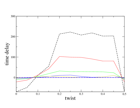
Figure 1: Time delay vs. twist for $\omega=0.86$ and $v$ ranging from 0.1 (dashed curve with larger amplitude) to 0.9 (dashed curve with smaller amplitude). The time delay for $v=0.9$ is at the $10^{-2}$ level though the dependence on twist is similar to that of the other curves.

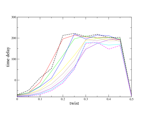
Figure 2: Time delay vs. twist for $v=0.1$ and $\omega$ ranging from $0.86$ (dashed curve with larger amplitude) to 0.95 (dashed curve with smaller amplitude).

III Scattering of many breathers

Now we consider the scattering of two trains of $N$ identical breathers. The total incoming energy has to be larger than the kink-antikink energy. With the kink and breather energies in Eqs. (14) and (18), we get the condition

$$8N\gamma\sqrt{1-\omega^{2}}>4$$ (26)

which translates into

$$N>\frac{1}{2}\sqrt{\frac{1-v^{2}}{1-\omega^{2}}}$$ (27)

This condition is simply an energy requirement.

The initial condition is a generalization of Eqs. (20)-(23)

$$\theta(t=0,x) = \sum_{j=1}^{N}\left[\theta_{b}(t=0,x;-x_{j},+v)+\theta_{b}(t=0,x;+x_{j},-v)\right]$$ (28)

$$\phi(t=0,x) = \pi\xi~{}{\rm tanh}(x/w)$$ (29)

$${\dot{\theta}}(t=0,x) = \sum_{j=1}^{N}\left[{\dot{\theta}}_{b}(t=0,x;-x_{j},v)+{\dot{\theta}}_{b}(t=0,x;+x_{j},-v)\right]$$ (30)

$${\dot{\phi}}(t=0,x) = 0$$ (31)

with

$$x_{j}=x_{0}+(j-1)a$$ (32)

where $x_{0}$ is the location of the innermost breather and $a$ is the spacing between the breathers in a train. An example of the initial condition is shown in Fig. 3.

With the initial conditions in terms of $\theta$ and $\phi$, we construct the vector field ${\hat{n}}(0,x)$ and its time derivative, $\partial_{t}{\hat{n}}(0,x)$. We then evolve ${\hat{n}}$ using Eq. (6), as discussed in greater detail in Appendix A. We hold the following parameters fixed in our numerical runs

$$N=4,\ \ \omega=0.95,\ \ x_{0}=32,\ \ a=\frac{4}{\eta\omega\gamma}=11.1,\ \ w=\frac{2}{\eta\omega\gamma}=5.55,$$ (33)

and $v\in[0,1]$ and $\xi\in[0,0.5]$ are scanned over. Most runs do not yield soliton creation but some runs do. An example of soliton creation occurs for $v=0.5$ and $\xi=0.1$, and is shown in Fig. 3. In Fig. 4 we mark the points in parameter space where we have found soliton creation. Note that non-zero twist is essential for soliton creation in this model.

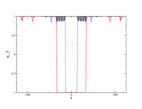
Figure 3: Three snapshots of the $z-$component of ${\hat{n}}$ for the run with $v=0.5$, $\xi=0.1$ and the remaining parameters as in Eq. (33). The initial breather state is the black solid curve. The final state is the solid (red) curve with the kink and the antikink interpolating between $n_{3}=+1$ and $n_{3}=-1$. An intermediate state is also shown (dashed blue curve).

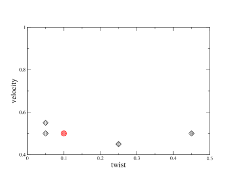
Figure 4: Diamonds indicate points in the velocity-twist plane where we have found soliton creation to occur with parameters as in Eq. (33). The point denoted by the filled circle corresponds to the parameters used in the successful kink creation shown in Fig. 3. Our numerical strategy scans in parameter space in steps of 0.05 in twist in the interval [0,0.5], and steps of 0.05 in velocity in the interval [0.4,0.95]. A more refined scan would fill in some of the parameter space though we expect a fractal distribution of parameters which successfully produce kinks Dutta:2008jt ; Romanczukiewicz:2010eg

It is worth pointing out that the outcome is sensitive to the choice of our fixed parameters in Eq. (33). Dependence on $N$ and the spacing $a$ is expected; but we also find dependence on $x_{0}$, suggesting that the phase of the breather trains on collision may be important in the outcome. This would be consistent with the chaotic nature of kink production in $\lambda\phi^{4}$ observed in Dutta:2008jt ; Romanczukiewicz:2010eg . In future work we are planning a more extensive scan of parameter space and to examine the chaotic nature of the scattering more closely ongoingwork .

IV Generalizations and Conclusions

The deformed O(3) sigma model suggests many generalizations that all seem worthwhile to explore.

The first generalization is to stay in 1+1 dimensions and to extend the model to an $N-$component vector. (This $N$ is not to be confused with the number of breathers in the previous section.) It may be possible to make some analytic advances by considering the kink creation problem in the large $N$ approximation. Other generalizations are to complexify the vector ${\hat{n}}$ and consider the CP(N) model, and to also include gauge fields.

The sigma model framework can be used to generalize to vortex and monopole formation, by simply choosing different potentials. We have already studied kink creation in the O(3) model with the potential

$$V({\hat{n}})=\frac{1}{2}[1-n_{3}^{2}]$$ (34)

To study vortex formation in 2+1 dimensions, it would be natural to choose

$$V({\hat{n}})=\frac{1}{2}[1-(n_{1}^{2}+n_{2}^{2})]$$ (35)

Now the true vacua lie around the equator of an $S^{2}$, and the vortex solutions correspond to either the northern or the southern hemisphere, and the center of the vortex will be either at the north or south poles. These two solutions are related by the $Z_{2}$ symmetry under $n_{3}\to-n_{3}$. In this model, we do not have a “twist” degree of freedom as in the kink case. Recall that in the kink case, we had a 1-parameter family of kink solutions labeled by the constant value of the azimuthal field $\phi$ as in Eq. (12). Similarly we need a one parameter family of vortex solutions and this can be obtained by extending the model to O(4). Then the vacua are still given by circles $n_{1}^{2}+n_{2}^{2}=1$ but there is a one parameter family of possible vortex solutions labeled by the angle in the $(n_{3},n_{4})$ plane.

A point to remember about vortices is that the energy of a global vortex-antivortex pair grows logarithmically with separation. So their creation is necessarily transient, unless the model is gauged. A similar comment applies to the creation of magnetic monopoles.

To study monopole formation in 3+1 dimensions in our O(3) model we would choose the potential,

$$V({\hat{n}})=\frac{1}{2}[1-(n_{1}^{2}+n_{2}^{2}+n_{3}^{2})]$$ (36)

except that this vanishes due to the constraint. The O(3) model does have the correct topology ($\pi_{2}(S^{2})=\mathbb{Z}$) for magnetic monopoles, but the monopoles are singular because there is no escape from the vacuum manifold. If we choose the potential in Eq. (36) but in an O(4) model, we get a situation similar to the vortex discussed above in the O(3) model: there are two non-singular monopole solutions corresponding to the two “hemispheres” in $S^{3}$. To include a twist similar to the one for kinks, we should go to at least an O(5) model, where the one parameter family of monopole solutions is labeled by the angle in the $(n_{4},n_{5})$ plane. However, monopoles can be relatively twisted even in the O(3) model and we now discuss this feature in greater detail.

Let us assume that a monopole is located at $z=+a$ and its asymptotic vector field ${\hat{n}}$ is given by Eq. (7) with $\theta=\theta_{+}$, where $\theta_{+}$ is the spherical angle measured from the $+z-$axis but with the origin of the coordinate system at $z=+a$. An antimonopole is now placed at $z=-a$ and its asymptotic field is given by

$${\hat{n}}=(\sin{\bar{\theta}}\cos{\bar{\phi}},\sin{\bar{\theta}}\sin{\bar{\phi}},\cos{\bar{\theta}})$$ (37)

with ${\bar{\theta}}=\pi-\theta_{-}$ where $\theta_{-}$ is the spherical angle measured from the $+z-$axis but with origin at $z=-a$. The azimuthal angle ${\bar{\phi}}=\phi+\alpha$ and $\alpha$ plays the role of the twist in the O(3) model.

In Ref. Taubes:1982ie Taubes used a Morse theory construction in the gauged O(3) model and proved the existence of a static solution consisting of a monopole and an antimonopole ($m{\bar{m}}$) separated by some distance. This is surprising because one expects the Coulombic $-1/r^{2}$ attractive force between the $m{\bar{m}}$) to bring them together, after which the two can annihilate. In Taubes’ solution, the $m{\bar{m}}$ are kept apart by a repulsive force provided by the “twist”. The result is an unstable solution since the monopoles can untwist, come together, and annihilate. The solution itself is quite complicated but has been found numerically in Refs. Ruber:1985 ; Kleihaus:1999sx .

A construction similar to the one used by Taubes exists in the electroweak model and the resulting $m{\bar{m}}$ solution is called the “sphaleron” Dashen:1974ck ; Manton:1983nd (for a review see Manton:2004tk ). The form of the sphaleron solution is spherically symmetric for a particular value of coupling constants and is known explicitly up to two simple profile functions given by ordinary second order differential equations. The solution has been studied numerically for a large range of coupling constants Kleihaus:1991ks ; Kunz:1989 ; Yaffe:1989ms .

A particularly convenient feature of the Morse theory construction, is that it provides a path from the $m{\bar{m}}$ solution to the vacuum. Thus the sphaleron decay path describes the annihilation of a twisted $m{\bar{m}}$ pair. As shown in Refs. Copi:2008he ; Chu:2011tx the decay products of the annihilation include electromagnetic fields with non-zero magnetic helicity, which is defined as

$${\cal H}=\int d^{3}x{\bf A}\cdot{\bf B}$$ (38)

The magnetic helicity, which measures the twisting and linking of magnetic field lines, is inherited from the initial twist in the $m{\bar{m}}$ pair that make up the sphaleron. The sphaleron decay analysis also shows that, after a short period of time, the evolution of the electroweak fields is such that magnetic helicity is conserved.

By a time reversal of the sphaleron decay process, we conclude that the convergence of electromagnetic helicity can possibly lead to the creation of sphalerons, and hence also $m{\bar{m}}$ with a relative twist. The twist may also provide the necessary repulsive force between monopoles and antimonoples so as to separate them and to prevent them from re-annihilating.

The usefulness of magnetic helicity may be conjectured based on another line of reasoning. In highly conducting plasmas it is known that magnetic helicity is a conserved quantity. The derivation goes as follows:

$$\frac{d{\cal H}}{dt} = \int d^{3}x\left[~{}\partial_{t}{\bf A}\cdot{\bf B}+{\bf A}\cdot\partial_{t}{\bf B}~{}\right]$$ (39)

$$= \int d^{3}x\left[({\bf E}+{\bf\nabla}A^{0})\cdot{\bf B}-{\bf A}\cdot{\bf\nabla}\times{\bf E}\right]$$

$$= \int d^{3}x\left[2{\bf E}\cdot{\bf B}+({\bf\nabla}A^{0})\cdot{\bf B}\right]$$

$$= \int d^{3}x\left[2{\bf E}\cdot{\bf B}-{A^{0}}{\bf\nabla}\cdot{\bf B}\right]$$

$$= 2\int d^{3}x\left[\left(\frac{\bf j}{\sigma}+{\bf v}\times{\bf B}\right)\cdot{\bf B}]\right]$$

$$\to 0$$

In the last two steps we have used Ohm’s law as applied to a plasma element moving with velocity ${\bf v}$. The electrical conductivity is assumed to be infinite, $\sigma\to\infty$, though there are arguments in support of helicity conservation even if $\sigma$ is finite but large. Crucially for us, in the second and fifth steps, we have had to assume the absence of magnetic monopoles and magnetic currents. Hence magnetic helicity is conserved in a highly conducting plasma provided there are no magnetic monopoles. Then we might expect that if magnetic helicity is externally driven to large values in a plasma of extremely high electrical conductivity, magnetic monopoles might be produced to cause the helicity to dissipate.

Our comments above also apply to the creation of sphalerons in the electroweak model since the sphaleron is precisely a bound state of an electroweak monopole and antimonopole. The monopole pair in the sphaleron are confined by a Z-string Achucarro:1999it and cannot escape. Hence, if a sphaleron is produced, it will later decay. The production and decay of a sphaleron can lead to baryon number violation. So the discussion above suggests that it may be possible to observe baryon number violation by focusing magnetic helicity in a dense plasma.

While we are still speculating, it is possible that the magnetic field of certain atomic nuclei contain non-trivial magnetic helicity: since magnetic helicity violates parity, the lightest stable candidate nuclei are ${\rm Li}^{7}$ and ${\rm Be}^{9}$ nucleardata . The scattering of a large number of such nuclei, $\sim 10^{3}$ based on energy requirements, seems like a possible path to concentrate magnetic helicity in a small spatial volume, perhaps sufficient to form a sphaleron. One way to investigate this process theoretically would be to use the description of nuclei in terms of Skyrmions. To study the feasibility of baryon number violation in the collision of “helical nuclei”, we would need to couple the Skyrmion fields to electroweak gauge fields, then consider the scattering of corresponding “helical Skyrmions” in an attempt to find in-states that lead to sphaleron production, and thus baryon number violation.

To conclude, we have studied the creation of solitons in a model that contains a twist degree of freedom in addition to the ones that are used for building the soliton. In our model in Sec. I, twist is an essential ingredient for the production of solitons because the dynamics in the zero twist sector is completely integrable. We have explicitly shown a range of parameters that lead to soliton creation. We have also discussed some applications of these ideas to the production of vortices and monopoles, and baryon number violation via the production of electroweak sphalerons.

Appendix A Numerical Notes

The most straightforward approach to solving the equations of motion is to use spherical coordinates as in Eqs. (9), (10). The issue there is that spherical coordinates are not globally well-defined and one must use two different patches, say, $(\theta_{z},\phi_{z})$ with respect to the $z-$axis and $(\theta_{x},\phi_{x})$ with respect to the $x-$axis. If $\theta_{z}$ becomes small, we can solve the evolution equation in terms of $\theta_{x}$ and $\phi_{x}$, and then transform to $\theta_{z}$ and $\phi_{z}$. We found that this scheme introduced unacceptable numerical errors in the boundary region of the two patches and we decided not to pursue this scheme.

Instead we decided to work with the vector representation (${\vec{n}}$) where the equation of motion can be written in first order form as

$$\partial_{t}{\vec{n}} = {\vec{m}}$$ (40)

$$\partial_{t}{\vec{m}} = \partial_{x}^{2}{\vec{n}}-[{\vec{m}}^{2}-(\partial_{x}{\vec{n}})^{2}]{\vec{n}}-n_{3}(n_{3}{\vec{n}}-{\vec{e}}_{3})$$ (41)

We evolved these equations using the explicit second order Crank-Nicholson method with two iterations Teukolsky:1999rm . We also implemented boundary conditions, though in practice our lattice was large enough that the boundaries were irrelevant.

The issue now is that when we discretize the above equations, they do not preserve the condition ${\vec{n}}^{2}=1$ and the orthogonality condition ${\vec{n}}\cdot{\vec{m}}=0$. To remedy this, we enforced these constraints at every time step by rescaling ${\vec{n}}$ so as to get a unit vector, and by subtracting out from ${\vec{m}}$ the component parallel to ${\hat{n}}$. To our satisfaction, this procedure conserved energy at the percent level and the evolution also remained stable.

References

- (1) S. Mandelstam, Phys. Rev. D 11, 3026 (1975).
- (2) S. Dutta, D. A. Steer and T. Vachaspati, Phys. Rev. Lett. 101, 121601 (2008) [arXiv:0803.0670 [hep-th]].
- (3) T. Romanczukiewicz and Y. Shnir, Phys. Rev. Lett. 105, 081601 (2010) [arXiv:1002.4484 [hep-th]].
- (4) S. V. Demidov and D. G. Levkov, JHEP 1106, 016 (2011) [arXiv:1103.2133 [hep-th]].
- (5) C. J. Copi, F. Ferrer, T. Vachaspati, A. Achucarro, Phys. Rev. Lett. 101, 171302 (2008). [arXiv:0801.3653 [astro-ph]].
- (6) Y. -Z. Chu, J. B. Dent, T. Vachaspati, Phys. Rev. D83, 123530 (2011). [arXiv:1105.3744 [hep-th]].
- (7) A. B. Zamolodchikov and A. B. Zamolodchikov, Annals Phys. 120, 253 (1979).
- (8) R. F. Dashen, B. Hasslacher, A. Neveu, Phys. Rev. D11, 3424 (1975).
- (9) M. Nishida, Y. Furukawa, T. Fujii, N. Hatakenaka, Phys. Rev. E80, 036603 (2009).
- (10) T. Vachaspati and P. Vaudrevange, in progress.
- (11) C. H. Taubes, Commun. Math. Phys. 86, 257 (1982). Commun. Math. Phys. 86, 299 (1982).
- (12) B. Rüber, Ph.D. thesis, University of Bonn, 1985.
- (13) B. Kleihaus, J. Kunz, Phys. Rev. D61, 025003 (2000). [hep-th/9909037].
- (14) R. F. Dashen, B. Hasslacher, A. Neveu, Phys. Rev. D10, 4138 (1974).
- (15) N. S. Manton, Phys. Rev. D28, 2019 (1983).
- (16) N. S. Manton, P. Sutcliffe, “Topological solitons,” Cambridge, UK: Univ. Pr. (2004) 493 p.
- (17) B. Kleihaus, J. Kunz, Y. Brihaye, Phys. Lett. B273 100 (1991).
- (18) J. Kunz and Y. Brihaye, Phys. Lett. B216 353 (1989).
- (19) L. G. Yaffe, Phys. Rev. D 40, 3463 (1989).
- (20) M. Hellmund and J. Kripfganz, Nucl. Phys. B 373, 749 (1992).
- (21) A. Achucarro, T. Vachaspati, Phys. Rept. 327, 347-426 (2000). [hep-ph/9904229].
- (22) E. Mottola and A. Wipf, Phys. Rev. D 39, 588 (1989).
- (23) http://www.nndc.bnl.gov/wallet/
- (24) S. A. Teukolsky, Phys. Rev. D61, 087501 (2000). [gr-qc/9909026].