A Community-Based Sampling Method Using DPL for Online Social Networks

Abstract

In this paper, we propose a new graph sampling method for online social networks that achieves the following. First, a sample graph should reflect the ratio between the number of nodes and the number of edges of the original graph. Second, a sample graph should reflect the topology of the original graph. Third, sample graphs should be consistent with each other when they are sampled from the same original graph. The proposed method employs two techniques: hierarchical community extraction and densification power law. The proposed method partitions the original graph into a set of communities to preserve the topology of the original graph. It also uses the densification power law which captures the ratio between the number of nodes and the number of edges in online social networks. In experiments, we use several real-world online social networks, create sample graphs using the existing methods and ours, and analyze the differences between the sample graph by each sampling method and the original graph.

I Introduction

As the number of people who use online social networks grows, there have been significant research interests on online social network analysis [1][2][3][4]. It is difficult and often impossible to analyze an online social network with millions of nodes in its entirety [5][6]. What we need is a sampling method that creates sample graphs that are representative of the original online social network [6][7][8][9].

A ‘good’ sample graph should be able to produce analytical results that would have been attained with the original graph. This means, the properties of a sample graph should be similar to those of the original graph. In this paper, we propose a new sampling method that satisfies a list of graph properties a ‘good’ sample graph should aim for. Given an original graph and a sample size, the proposed sampling method creates a sample graph with the properties quite similar to the original graph.

Existing graph sampling methods are classified into three groups [6]: sampling methods by random node selection, sampling methods by random edge selection, and sampling methods by exploration. Sampling methods by random node selection create a sample graph by selecting a set of nodes and then including the edges connecting the selected nodes. Sampling methods by random edge selection create a sample graph by selecting a set of edges and then including the nodes connected to the selected edges. Sampling methods by exploration create a sample graph by selecting a seed node uniformly at random, exploring the neighbor nodes, selecting the nodes explored and the edges connecting them, and continuing to explore more nodes [6].

We claim that existing graph sampling methods fail to create samples that retain the properties of an original graph. In the existing graph sampling methods, the sample size is determined either by the number of nodes or by the number of edges. The sampling methods by random node selection or by exploration repeatedly select nodes until satisfying the given number of nodes without regard to the number of edges. The sampling methods by random edge selection, on the other hand, repeatedly select edges until satisfying the given number of edges without regard to the number of nodes. As a result, a sample graph may have the node-edge ratio quite different from that of the original graph since the sample size is determined by a single basis. Furthermore, the sampling methods by exploration create a sample graph that reflects the properties of only the part of the original graph (near the seed node where sampling is taken place). Finally, the random selection inherent employed in existing graph sampling methods tends to generate ‘random’ samples; the properties of sample graphs tend to be inconsistent with one another and with the original graph.

In this paper, we propose a new sampling method based on two key concepts: hierarchical community extraction and Densification Power Law (DPL). The hierarchical community extraction partitions the original graph into a set of densely-connected sub-graphs (i.e., communities), and uses a dendrogram to represent the hierarchy between the set of communities [10][11][12]. A set of sample sub-graphs, one for each community, is created by selecting nodes within the community with the probability of selecting a node to be in proportion to its degree and by selecting edges connecting them. The final sample graph is created by merging the sample sub-graphs while retaining the connectivity across the communities using the dendrogram. The Densification Power Law (DPL) represents the ratio between the number of nodes and the number of edges in real-world social networks [5]. When creating a sample sub-graph, we use the ratio between the number of nodes and the number of edges given by the DPL as a guideline.

By combining hierarchical community-based sampling and DPL, we overcome the problems with existing sampling methods. First, since the method uses the DPL, the sample graph created by the proposed method reflects the ratio between the number of nodes and the number of edges in both local and entire regions of the original graph. Second, since the method uses the hierarchy community extraction, the sample graph reflects the topology of the original graph well. Third, since the method considers both the topology and the node-edge ratio of the original graph, the properties of sample graphs obtained from the same original graph tend to be consistent with one another and with the original graph.

Through experiments on several diverse real-world online social networks, we demonstrate the effectiveness of our sampling method. As a performance metric, we use five well-known properties of a social network: degree distribution, singular value distribution, singular vector distribution, average clustering coefficient distribution, and hop distribution. The difference between several existing methods and ours is evaluated using K-S D-statistics (Kolmogorov-Smirnov D-statistics) [6]. The analyses show that the properties of the sample graph by our method are the most similar to those of the original graph.

The paper consists of the following. Section II introduces existing sampling methods and points out the problems with the existing methods. Section III describes the proposed method and presents the detailed process. Section IV compares the performance of the proposed methods with those of the existing methods through experiments. Section V summarizes and concludes the paper.

II Related Work

In this section, we review the existing sampling methods and point out their problems.

II-A Existing Sampling Methods

Leskovec and Faloutsos classified the sampling methods into three groups: sampling methods by random node selection, sampling methods by random edge selection, and sampling methods by exploration [6]. Figure 1 shows an example of the sampling methods by random node selection. The nodes and edges with solid lines are the ones selected for the sample graph, and those with dashed lines are the ones not selected. The sample graph in Figure 1 is created by selecting a set of nodes uniformly at random and then by selecting all of the edges connecting the selected nodes. If the sample size is given, the method selects nodes repeatedly until satisfying ‘the number of nodes’ to be selected for the sample.

Sampling methods based on random node selection differ in the way nodes are selected. Random Node (RN) sampling selects a set of nodes uniformly at random. The sample graphs created by RN are expected to reflect the properties of the original graph, as samples are selected from the entire population space. In Random Degree Node (RDN) sampling, the probability of a node being selected is proportional to its degree. In Random PageRank Node (RPN) sampling, the probability of a node being selected is proportional to the authority score computed by PageRank [13]. The idea behind RDN and RPN is to increase the chance of including ‘important’ nodes in a sample graph. The nodes with many edges, the hubs, are the important nodes in a social network and should be included in a sample graph [14].

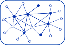
Figure 1: Sampling methods by random node selection.

Figure 2 shows an example of the sampling methods by random edge selection. The sample graph in the figure is created by selecting a set of edges uniformly at random and then selecting all of the nodes connected to the selected edges. If the sample size is given, the method selects edges until satisfying ‘the number of edges’.

Similar to sampling methods by random node selection, sampling methods by random edge selection differ in the way edges are selected. Random Edge (RE) sampling selects a set of edges uniformly at random and all the nodes connected to the selected edges. The sample graphs created by RE tend not to reflect the structure of the original graph since the high-degree nodes are selected more frequently. Random Node Edge (RNE) sampling solves the problem by selecting a node uniformly at random and then selects an edge uniformly at random among the edges connected to the selected nodes [6].

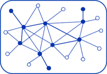
Figure 2: Sampling methods by random edge selection.

The sampling methods by exploration create a sample graph by selecting a seed node uniformly at random, exploring its neighbor nodes, selecting all of the nodes explored and their connecting edges, and continuing to explore more nodes. If the sample size is given, the method selects nodes repeatedly from the original graph until satisfying ‘the number of nodes’.

Depending on which edges to include in the sample, the exploration methods are further classified into two: non-induced and induced. The non-induced method includes only the edges explored in the sample graph. The induced method includes not only the explored edges but all of the edges connected to the selected nodes [7]. Figure 3 shows the examples of sampling methods by exploration. The node $S$ is a seed node. The method creates a sample graph by exploring the nodes connected to the seed node, as shown in Figure 3.

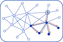
Figure 3: Sampling methods by exploration.

Sampling methods by exploration include Random Walk (RW) sampling, Random Jump (RJ) sampling, and Forest Fire (FF) sampling. Both RW and RJ sampling methods use the concept of random walk with restart [13]. The difference is the number of seeds used. RW sampling uses a single seed node; RJ sampling uses a set of seed nodes. Compared to RW and RJ that explores the graph depth-first, FF sampling explores the graph breadth-first. FF sampling picks a seed node at random, explores not a single but multiple neighbor nodes. Then, it continues to explore the nodes connected to the explored neighbor nodes recursively.

II-B Problems of Existing Sampling Methods

We point out problems of the existing sampling methods by group. First, sample graphs created by random node selection may have more or fewer ‘edges’ than the number of edges estimated by the ratio between nodes and edges of the original graph, since the sampling methods select nodes until satisfying the estimated number of nodes without regard to the number of edges. For example, suppose that sample size is 10%, the number of nodes of original graph is 5,000, and the number of edges of the graph is 10,000. The sample graph should have 500 nodes and about 800 edges (In social networks the number of edges tends to decrease exponentially when the number of nodes increases linearly. In Section III, we will explain it in detail). Sampling methods by random node selection do not meet this requirement.

Most random node selection methods select nodes at random. The random selection tends to generate ‘random’ samples; the properties of the resulting graphs sampled from the same original graph tend to be inconsistent with one another and with the original graph. RDN and RPN do not select nodes at random but select nodes in proportion to their degrees or authority scores. Sample graphs created by RDN and RPN are more consistent, but they tend to be denser than the original graph since they include many high-degree nodes.

Second, similar to the cases with random node selection, sample graphs created by random edge selection may have more or fewer ‘nodes’ than the estimation provided by the ratio between nodes and edges of the original graph. Also, the properties of the resulting sample graphs created by random edge selection tend to be inconsistent with one another and with the original graph since most methods select edges at random.

Third, sampling methods by exploration repeatedly select nodes until satisfying the estimated number of nodes, as done in random node selection. Thus, similar to the cases with random node selection, sampling by exploration may have more or fewer edges than the estimation provided by the ratio between nodes and edges of the original graph. The node-edge ratio of the sample graph created by the non-induced method is closed to 1:1 since only the explored nodes and edges are selected. The node-edge ratio of the sample graph created by the induced method, on the other hand, is not 1:1 since the explored nodes and all of the edges connecting the selected nodes are selected. When all of the edges connecting the nodes in the connected graph are included into the sample graph as in the induced methods, however, the sample graph would be denser than the original graph. Also, the sample graphs created by exploration are inconsistent since the methods select seed nodes at random and the neighbor nodes of the seed node at random.

Furthermore, sample graphs created by exploration do not represent entire graph but only the part near the seed node. RJ is regarded as a solution to this problem. Sample graphs created by RJ reflect the properties of the various quarters of the original graph better because it uses multiple seeds.

III Proposed method

In this section, we propose a new sampling method and describe its process in detail.

III-A Overview

In the previous section, we have pointed out the problems with existing sampling methods. The new sampling method is designed to achieve the following:

(a)	The sample graph should reflect the node-edge ratio of each region of the original graph.
(b)	The sample graph should reflect the node-edge ratio of the entire original graph.
(c)	The sample graph should reflect the topology of each region of the original graph.
(d)	The sample graph should reflect the topology of the entire graph.
(e)	The properties of graphs sampled from the same graph by the proposed method should be consistent with one another.

The properties of regions of a social network may be different from one another and also from those of the entire network. If we create a sample graph which reflects the node-edge ratio of the entire graph only, the node-edge ratio of a region of the sample graph may not correctly represent its corresponding region of the original graph. The properties of a graph are closely associated with the topology of the graph. Thus, we should create a sample graph which reflects both the topology of each region and the entire graph. Finally, we should create sample graphs from the same graph whose properties are consistent with one another and with the original graph.

To create a sample graph that reflects the properties of the original graph, the proposed sampling method utilizes two key concepts: hierarchical community extraction and Densification Power Law (DPL). First, it uses hierarchical community extraction to partition the original graph into a set of densely-connected sub-graph, i.e., communities. Hierarchical community extraction not only partitions the original graph into a set of communities but also creates a dendrogram that represents the partition hierarchy. Figure 4 shows an example of the dendrogram. The large circle is the community, and the edge among the circles represents the parent-child relationship between communities. In Figure 4, a parent community is partitioned into two children communities. After partitioning the original graph into a set of communities, the proposed method builds sample sub-graphs, one for each community. Then, the method merges sub-graphs into a final sample graph from bottom up, while taking the connections between the communities into account using the dendrogram.

Second, the proposed method uses the DLP, when determining the number of nodes and edges to be included in each sample sub-graph. The DLP states that the number of nodes and the number of edges in a social network follows the power law distribution [5]. Equation 1 shows DPL. In Equation 1, $e$ represents the number of edges, and $n$ does the number of nodes. Typically, densification exponent $\alpha$ takes the value between 1 and 2.

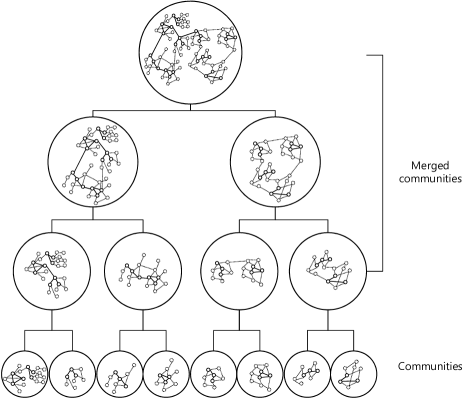
Figure 4: A dendrogram and the process of the proposed method.

$$e\propto n^{\alpha}$$ (1)

In the existing sampling methods, the sample size is based on either the number of nodes or the number of edges (but not both). In comparison, the proposed method uses DPL when determining the size of the sample graph. The proposed method estimates the number of sample edges using DPL when the sample size is given as the number of nodes in a social network. The proposed sampling method first determines the value of $\alpha$ for each sub-graph (i.e., community) in the original graph based on the number of edges and nodes within it. It determines the number of nodes to be included in a sample community based on the number of nodes in its corresponding community in the original graph. Then, it computes the number of edges in the sample community by using the value of $\alpha$ for its corresponding original community. A similar approach is used when the sample size is given as the number of edges.

In summary, the proposed sampling method works as follows. First, the method partitions the original graph into sub-graphs. Second, it computes the densification exponent $\alpha$ based on the number of nodes and edges for every community in the original graph. Third, it builds sample sub-graphs by selecting nodes in proportion to their degrees and edges connecting the selected nodes. The node-edge ratio in a community is controlled by $\alpha$. Finally, it merges sample sub-graphs into a final sample graph in a bottom up fashion, while taking the connections between communities into account. For each merged community, the node-edge ratio is also controlled by $\alpha$ of its corresponding community in the original graph. Figure 4 shows the process of the proposed method. The nodes and edges in a community with dashed lines are the ones not selected in the sample graph, and those with solid lines are the ones selected in the sample graph.

III-B Process of the proposed method

In this section, we explain the process of the proposed method in detail.

III-B1 Determining the number of sample nodes and sample edges

The number of sample nodes and the number of sample edges in each community are determined as follows. First, the proposed method computes the number of sample nodes based on the sample size. Second, based on the densification exponent $\alpha$, the method computes the number of edges to be selected from each community. This process makes sure that the sample graph reflects the node-edge ratio in each community. For example, suppose the sample size is 10%, the number of nodes and edges of in the original graph are 500 and 1000, respectively. Based on equation (1), the densification exponent $\alpha$ of the original graph is 1.11. The number of sample nodes and sample edges from that community are 50 and 76, respectively.

All the nodes in the original graph exist within the communities, but some edges in the original graph exist between the communities. Thus, we must determine the number of edges to be selected between two communities (i.e., inter-community edges). The method determines the number of edges to be selected between two child communities as the difference between the number of edges to be selected from the parent community and the number of edges to be selected from two child communities. This provides the number of inter-community edges to be selected between the two communities.

III-B2 Sampling with communities

The proposed method creates a sample graph from each community as follows. First, it selects nodes from each community until satisfying the number of sample nodes pre-determined by the sample size. Similar to RDN, the probability of selecting a node is in proportion to its degree, which ensures important nodes are selected. Second, it selects edges until satisfying the number of edges determined by DPL. The probability of selecting an edge is proportional to the sum of the degrees of the nodes connected to it. Sample graphs created by this method are more consistent with one another since the method selects high-degree nodes as in RDN. Also, since the degree of nodes conveys topological information, each sample sub-graph created by this method reflects the topology of each sub-graph of the original graph.

Finally, the method creates the final sample graph by sampling edges among communities in the reverse order of partition of the original graph using hierarchical community extraction. There exist a few edges that connect two communities. In social network analysis, these few edges are defined as weak-tie [14]. The method selects the inter-community edges in proportion to the sum of degrees of nodes connected to it, similar to the way it selects edges within the community.

The proposed method may use any hierarchical community extraction method as long as it provides a dendrogram. We use the method which automatically determines the number of communities to be extracted, such as the modularity-based algorithm [10][12] and cross-association (CA) [15]. Of course, one may use the method which requires the number of communities as an input, such as METIS [16] and chameleon [17], as long as domain experts supply the optimal number of communities. In this paper, we have used the modularity-based algorithm, a well-known hierarchical community extraction method [10][12].

IV Experiments

In this section, we demonstrate the effectiveness of the proposed method by comparing it with several existing sampling methods.

IV-A Experimental Setup

We use seven real-world online social networks in our experiments [18][19][20][21][22]. First, ‘Wiki-vote’ is a dataset collected from Wikipedia from the day when the service opened to Jan 2008. A node represents a user of Wikipedia, and an edge represents a recommendation between the users. Second, ‘Email Enron’ is a collection of emails from Enron. A node represents an email address, and an edge represents a communication between email addresses. Third, ‘Epinions’ is a dataset collected from epinions.com, a product review website. A node represents a user, and an edge represents a recommendation between the users. Fourth and fifth, ‘Hep_ph’ (High Energy Physics-Phenomenology) and ‘Hep_th’ (High Energy Physics-Theory) are the datasets from Arxiv website, a website that collected unpublished papers, from Jan 1992 to Apr 2003. In both datasets, a node represents a paper, and an edge represents a reference between papers. Sixth, ‘AS’ is a dataset collected from the log analysis of border gateway protocol between the Autonomous Systems, from Nov 1997 to Jan 2000. A graph of routers comprising the Internet can be organized into sub-graphs called Atonomous System (AS). A node represents an AS, and an edge represents a communication between ASs. Seventh, ‘Oregon’ is a log data collected from Oregon routers, from Mar 2001 to May 2001. A node represents a router in Oregon, and an edge represents a communication between the routers. We generate undirected graphs with these data. Table 1 shows the numbers of nodes and edges in each dataset.

TABLE I: The size of the dataset used in the experiments

	# of nodes	# of edges
Wiki-vote	7,115	201,524
Email Enron	36,692	367,662
Epinions	75,879	811,480
Hep_ph	34,545	841,754
Hep_th	27,768	704,570
AS	6,743	25,144
Oregon	10,669	44,004

As performance metric, we use a set of five well-known graph properties: degree distribution, singular value distribution, singular vector distribution, average clustering coefficient (CC) distribution and hop distribution [6]. The degree distribution is the distribution of the number of nodes with degree $d$ for every degree $d$. The degree distribution of an social network typically follows a power law distribution [2]. The singular value distribution and the singular vector distribution are the distributions computed by singular value decomposition (SVD) of the graph adjacency matrix [23]. These two properties represent the characteristics of the community structure of a graph. The average CC distribution is the distribution of the average CC of nodes for every degree $d$. The CC of a node is the ratio between the number of edges among the node and neighbor nodes and the number of possible edges among the node and neighbor nodes. If the number of neighbors of a given node is $k$, the number of possible edges is $\frac{(k(k-1))}{2}$. The hop is the minimum distance between two nodes. The hop distribution is the distribution of the number of reachable pairs in hop $h$ for every hop $h$ [2].

The sampling methods compared in our experiments are the proposed method, RN, RDN, RPN, RE, RNE, RW, RJ, and FF. We use both the non-induced versions of RW, RJ, and FF, and the induced versions of RW (RW(i)), RJ (RJ(i)), and FF (FF(i)), respectively. The proposed method is denoted as ‘C+D’ (Community + DPL). We set the probability of restart to be 0.15 for RW and RJ. For FF, we set $P_{f}$ to be 0.3, the best value suggested in [6]. In all methods, we use the sample size of 10%.

IV-B Performance comparisons

In this section, we compare the performance of the proposed method with other sampling methods. First, we visually inspect the CC and degree distributions. Second, we examine the performance of various sampling methods more rigorously using K-S D-statistics. Third, we check the consistency among the graphs sampled from the same original graph by each sampling method. Finally, we examine the densification exponent of each sampling method.

IV-B1 CC and degree distributions

We examine how well the sample graph reflects the properties of the original graph. The evaluation is based on visual inspection on the CC distributions and degree distributions of the sample graphs by various sampling methods. The comparison between the other distributions of the original graph and those of the sampling methods are not presented since they show no visible difference.

Figure 5 depicts the CC distribution of the original graph and that of each sampling method. In Figure 5, the x-axis represents the degree of nodes, and the y-axis represents the CC of nodes. The CC distribution of the original graph is similar to that of the sample graph created by the proposed method. The CC distributions of the sample graphs created by RDN, induced FF, and induced RW are also similar to that of the original graph. The CC distributions of the sample graphs created by RN and RE, however, are quite different from that of the original graph.

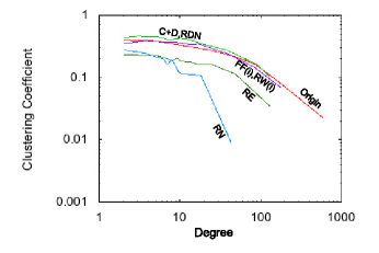
Figure 5: CC distributions of the original graph and the sample graphs.

Figure 6 shows the degree distribution of the original graph and the sample graphs created by various sampling methods. In Figure 6, the x-axis represents the degree of nodes, and the y-axis represents the number of nodes. Again, the shape of the degree distribution of the original graph is similar to that of the sample graph created by the proposed method. The degree distribution of the sample graph created by RN is similar to that of the original graph, but those by the other methods are quite different from that of the original graph. The visual inspection suggests that the propose method creates a sample graph with the properties most similar to those of the original graph.

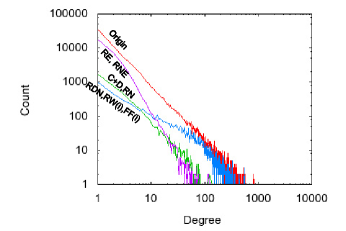
Figure 6: Degree distributions of the original graphs and the sample graphs.

IV-B2 K-S D-statistics

We compute the difference between the five properties of the original graph and those of the sample graph using K-S D-statistics (Kolmogorov-Smirnov D-statistics). K-S D-statistics computes the maximum difference between the cumulative distribution function of the original graph and that of the sample graph (see Equation (2)). The $D$ value computed by K-S D-statistics is between 0 and 1. As the value approaches 0, the property of the sample graph is more similar to that of the original graph.

$$D=max_{x}(|F(x)-F^{\prime}(x)|)$$ (2)

The size of a sample graph matters; The closer the size of a sample graph is to that of the original graph, the more the properties of the sample graph are similar to those of the original graph [6]. For fair comparison, therefore, we should use sample graphs with the same number of nodes or edges. However, the existing sampling methods determine the size of a sample graph using either the number of nodes or the number of edges. Thus, node-based methods and edge-based methods could not be compared fairly since the number of nodes and edges of the sample graphs created by each sampling method could not be standardized. The proposed method can be compared fairly with both node-based and edge-based sampling methods. Thus, we separate the comparisons into two groups: the comparison between the proposed method and node-based sampling methods and the comparison between the proposed method and edge-based sampling methods. We create 10 sample graphs by each sampling method and then compute the average of the D-statistics of the sample graphs.

Tables 2 and 3 show the comparison of the proposed method and node-based sampling methods and the comparison of the proposed method and edge-based sampling methods, respectively. In Tables 2 and 3, the numbers between 0 and 1 represent the D-statistics for five different properties, and $R$ represents the ranking of the sampling methods. $Avg$ represents the average of the five D-statistics.

As shown in Tables 2 and 3, the performance of the proposed method is consistently higher than those of existing sampling methods. In Table 2, the proposed method is ranked high in all properties except hop distribution. In degree distribution and singular value distribution properties, where the proposed method is ranked the first, the difference between the D-statistic values of the top and the second is quite significant. In comparison, the D-statistics values of hop distribution, where the proposed method is ranked the sixth, all of the sampling methods are quite similar. Thus, the sample graph created by the proposed method reflects the properties of the original graph the best. In particular, the sample graph created by the proposed method reflects the degree, singular value, and singular vector distributions of the original graph well. This is because the proposed method creates a sample graph by selecting nodes and edges in proportion to their degrees and using the hierarchical community extraction. Note that the D-statistics value of CC of non-induced FF is 1. Since non-induced FF selects only the explored nodes and edges and does not explore the explored nodes again, the sample graph created by non-induced FF is a tree, which results in a significant difference in the CC distribution of non-induced FF and that of the original graph. In Table 3, the proposed method is ranked the first in all properties.

In Tables 2 and 3, the variance of D-statistics in each property differs. When comparing the performance of the sampling methods using the average D-statistics of five properties, the overall ranking depends on the D-statistics with wide variation. To avoid this problem, we also compare the performance of the sampling methods by normalizing the D-statistics. We normalize the D-statistics values of each property by min-max normalization [24]. The numbers in parentheses in Tables 2 and 3 refer to normalized values and ranks computed with the normalized values. The proposed method outperforms the other sampling methods. The difference between the average score of the top and the second with normalization is larger than that obtained without normalization.

TABLE II: The proposed method vs. node-based sampling methods

	Degree	R	Sval	R	Svec	R	CC	R	Hop	R	Avg	R
C+D	0.132	1	0.044	1	0.176	2	0.338	3	0.045	6	0.147 (0.041)	1 (1)
RN	0.229	2	0.138	8	0.211	5	0.402	7	0.047	7	0.205 (0.257)	6 (6)
RDN	0.258	5	0.085	3	0.215	6	0.367	4	0.032	2	0.191 (0.172)	2 (3)
RPN	0.256	4	0.091	5	0.175	1	0.379	5	0.027	1	0.186 (0.166)	3 (2)
RW	0.229	2	0.128	7	0.189	4	0.470	8	0.052	8	0.214 (0.260)	7 (7)
RJ	0.353	9	0.183	10	0.436	9	0.592	9	0.044	5	0.322 (0.502)	9 (9)
FF	0.309	8	0.142	9	0.860	10	1.000	10	0.215	10	0.505 (0.836)	10 (10)
RW(i)	0.293	6	0.088	4	0.223	7	0.335	2	0.036	3	0.195 (0.193)	5 (4)
RJ(i)	0.506	10	0.104	6	0.185	3	0.380	6	0.036	4	0.242 (0.381)	8 (8)
FF(i)	0.305	7	0.084	2	0.265	8	0.260	1	0.058	9	0.195 (0.210)	4 (5)

TABLE III: The proposed method vs. edge-based sampling methods

	Degree	R	Sval	R	Svec	R	CC	R	Hop	R	Avg	R
C+D	0.128	1	0.041	1	0.187	1	0.303	1	0.042	1	0.140 (0)	1 (1)
RE	0.258	2	0.130	2	0.349	2	0.360	2	0.054	2	0.230 (0.586)	2 (2)
RNE	0.302	3	0.143	3	0.580	3	0.518	3	0.061	3	0.320 (1)	3 (3)

IV-B3 Consistency of sample graphs

In this set of experiments, we evaluate the consistency of various sampling methods. The consistency is measured by the standard deviation of D-statistics of sample graphs. As shown in Table 4, the standard deviation of RDN is the lowest, followed by RPN, the proposed method, and RE. Note that the average standard deviations of lower-ranked sampling methods are quite high. Since RDN and RPN select high-degree nodes, the sample graphs tend to be consistent. RE also selects many high-degree nodes, because it includes the nodes connected to selected edges into the sample graph though edges are selected at random. Thus, the sample graphs created by RE tend to be consistent. The sample graphs created by the proposed method are consistent since it selects nodes and edges in proportion to their degree like RDN and RPN. The sample graphs created by the proposed method is somewhat less consistent than those of RDN and RPN, because RDN and RPN select all of the edges connected to selected nodes while the proposed method selects edges in proportion to degree of nodes connecting the edges. The proposed method generates consistent sample graphs and ranked the third among various sampling methods.

TABLE IV: Standard deviation of the sample graphs created by various sampling methods

	Degree	R	Sval	R	Svec	R	CC	R	Hop	R	Avg	R
C+D	0.0002	3	0.0001	7	0.0021	7	0.0005	3	0.0004	6	0.0006	3
RN	0.0053	10	0.0050	11	0.0093	9	0.0230	12	0.0006	10	0.086	10
RDN	0.0002	2	0	3	0.0002	1	0.0003	2	0.0002	1	0.0002	1
RPN	0.0003	4	0	5	0.0002	2	0.0006	4	0.0003	3	0.0003	2
RE	0	1	0	2	0.0003	3	0.0020	6	0.0004	5	0.0006	3
RNE	0.0004	6	0	1	0.0113	10	0.0026	7	0.0004	7	0.0029	8
RW	0.0072	11	0.0007	9	0.0056	8	0.0207	11	0.0005	9	0.0069	9
RJ	0.0004	5	0.0001	6	0.1020	11	0.0109	10	0.0003	4	0.0228	11
FF	0.0092	12	0.0125	12	0.8637	12	0	1	0.0048	12	0.1780	12
RW(i)	0.0024	9	0.0005	8	0.0014	4	0.0070	9	0.0005	8	0.0024	6
RJ(i)	0.0005	7	0	4	0.0018	6	0.0008	5	0.0002	2	0.0007	5
FF(i)	0.0020	8	0.0015	10	0.0016	5	0.0068	8	0.0008	11	0.0025	7

IV-B4 Densification exponent

The sampling target in this paper is a social network. Thus, the ratio of the number of nodes and the number of edges in the sample graph should follow the DPL. In this set of experiments, we examine whether the sample graphs reflect the node-edge ratio of the original graph. Table 5 shows the difference between the densification exponent of the sample graph created by each sampling method and that of the original graph.

TABLE V: Difference between the densification exponent of the sample graph and that of the original graph

Sampling method	difference
C+D	0.033
RN	-0.063
RDN	0.135
RPN	0.104
RE	-0.065
RNE	-0.162
RW	-0.096
RJ	-0.142
FF	-0.156
RW(i)	0.141
RJ(i)	0.105
FF(i)	0.149

The sample graph created by the proposed method reflects the node-edge ratio of the original graph more than the others. The result is not surprising since the proposed method takes into account the node-edge ratio of the original graph when creating a sample graph. Of course, the node-edge ratio of the sample graph created by the proposed method is not exactly the same as that of the original graph. It is because the proposed method uses not the node-edge ratio of the entire graph but the node-edge ratio of each partitioned sub-graph.

The node-edge ratios of the sample graphs created by RN and RE are slightly lower than that of the original graph. In the case of RN, because sample nodes are selected uniformly at random from the entire population space, the selected nodes often do not have edges between them. Similarly, in the case of RE, because sample edges are selected uniformly at random from the entire population, the nodes connected to the selected edges often form an island. In both cases, RN and RE end up with a sample graph sparser than the original graph. RNE is the lowest, because RNE tries to avoid the problem that RE selects many high-degree nodes. In contrast, the node-edge ratio of the sample graphs created by RDN and RPN is much higher than that of the original graph because RDN and RPN select many high-degree nodes.

The sample graphs created by non-induced RW, RJ, and FF are much lower than that of the original graph because the method selects only explored nodes and edges. In contrast, the sample graphs created by induced RW, RJ, and FF are denser than that of the original graph because they select not only explored nodes and edges but also all of edges connecting selected nodes. RJ uses multiple seed nodes while RW and FF use a single seed node. Thus, the node-edge ratio of the sample graph created by RJ is lower than those of RW and RJ even though that of the sample graph created by RJ is denser than that of the original graph

IV-C The effectiveness of the techniques used in the proposed method

In the previous section, we have shown that the proposed method outperforms the other sampling methods. As the proposed method is based on two techniques, community-based sampling and DPL-based sampling, we examine the effectiveness of these two techniques.

IV-C1 The effectiveness of community-based sampling

First, we examine the effectiveness of the community-based sampling technique when creating a sample graph that reflects the properties of the original graph. We apply the community-based sampling technique to the existing sampling methods and evaluate the performance of the sampling methods with community-based sampling.

For experiments, four representative sampling methods are selected: RN for sampling by random node selection, RE for sampling by random edge selection, RW for sampling by exploration, and RDN whose selection process is similar to that of the proposed method. We call RN, RE, RW, and RDN with community-based sampling as community-based RN, community-based RE, community-based RW, and community-based RDN, respectively. To apply the community-based method to the existing sampling methods, we have done the following. The community-based RN selects nodes at random from each community partitioned by hierarchical community-extraction method and then selects all of edges connecting the selected nodes. The community-based RE selects edges at random from each community and then selects all of nodes connected to the selected edges. The community-based RDN selects nodes in proportion to the degree of a node from each community and then selects all of edges connecting the selected nodes. The community-based RW selects a seed node from each community and then selects all of nodes explored by exploring neighbors of the seed node. It selects all of edges connecting selected nodes. The experimental setup and method are the same as those in Section IV.B.2.

Table 6 compares the performance of the existing methods with and without the application of community-based sampling. In Table 6, ‘CBased’ represents a method with community-based sampling. Table 6 confirms that the community-based sampling methods outperform the original sampling methods.

Community-based sampling makes the sample graph to reflect the topology of the original graph better. For example, the nodes in a community are densely connected to each other. Thus, if community-based RN selects nodes and edges in a community, the nodes in the sample graph can be thought densely connected to each other. Thus, community-based RN creates a sample graph that reflects the properties of the original graph better than RN. The performance of all community-based sampling methods improves for a similar reason. We conclude community-based sampling is an effective technique for creating a sample graph which reflects the properties of the original graph.

TABLE VI: Comparison of the sampling methods with and without community-based sampling

	Degree	Sval	Svec	CC	Hop	Avg
RN	0.289	0.138	0.211	0.402	0.047	0.217
CBasedRN	0.273	0.112	0.207	0.372	0.052	0.203
RDN	0.549	0.085	0.215	0.367	0.032	0.250
CBasedRDN	0.537	0.085	0.198	0.384	0.035	0.248
RE	0.210	0.130	0.349	0.360	0.054	0.220
CBasedRE	0.188	0.118	0.339	0.359	0.031	0.207
RW	0.540	0.128	0.189	0.470	0.052	0.269
CBasedRW	0.487	0.090	0.188	0.321	0.037	0.225

IV-C2 The effectiveness of DPL-based sampling

In this section, we examine the effectiveness of the DPL-based sampling technique for creating a sample graph that reflects the properties of the original graph. We apply the DPL-based sampling technique to the existing sampling methods and evaluate the performance of the sampling methods with and without DPL-based sampling.

Similar to the previous experiments, we use RN, RE, RW, and RDN as representative sampling methods. We should make sure the node-edge ratio of the sample graph is the same as that of the original graph. A simple way to achieve this would be to create a sample graph by the original method and then include or remove edges to match the node-edge ratio. Note that the inclusion or removal of nodes would not make the sample graph with the desired node-edge ratio because when nodes are removed, edges connecting the removed nodes are removed automatically. Thus, we insert or remove only ‘edges’ from the sample graph created by the existing method. The number of edges in the sample graph created by RN, RE, and RW are less than the number of edges computed by the node-edge ratio of the original graph. Thus, DPL-based RN, RE, and RW include more edges in proportion to the sum of degrees of two nodes connected to the edges. DPL-based RDN retains the edges in proportion to the sum of degrees of two nodes connected to the edges and removes the rest. The experimental setup and method are equal to those of Section IV.B.2.

Table 7 compares the existing sampling methods with and without DPL-based sampling. In Table 7, ‘DBased’ represents a method with DPL-based sampling. Compare to Table 6, Table 7 shows that not all of the DPL-based sampling methods outperform the original sampling methods. DPL-based RW and DPL-based RDN are better than original RW and RDN, respectively, while original RN and RE are better than DPL-based RN and DPL-based RE, respectively. From these results, one may conclude the DPL-based sampling technique is not effective. This conclusion, however, is incorrect. community-based RDN can be viewed as the proposed method without DPL-based sampling. When we compare the performance of community-based RDN (in Table 6) and that of the proposed method (in Table 2), the proposed method is better than community-based RDN, which indicates the DPL-based sampling technique is effective in the proposed method. A more correct interpretation of the results in Table 7 is that it is difficult to apply DPL-based sampling to those methods. The simple inclusion or removal of edges to the sample graph created by the existing methods fails to keep the key concept of each sampling method.

TABLE VII: Comparison of the sampling methods with and without DPL-based sampling

	Degree	Sval	Svec	CC	Hop	Avg
RN	0.289	0.138	0.211	0.402	0.047	0.217
DBasedRN	0.430	0.160	0.355	0.478	0.215	0.328
RDN	0.549	0.085	0.215	0.367	0.032	0.250
DBasedRDN	0.343	0.312	0.267	0.266	0.028	0.243
RE	0.210	0.130	0.349	0.360	0.054	0.220
DBasedRE	0.395	0.062	0.526	0.717	0.258	0.392
RW	0.540	0.128	0.189	0.470	0.052	0.269
DBasedRW	0.348	0.290	0.259	0.230	0.028	0.231

IV-C3 The performance of the proposed method with different densification exponent

We have not been able to conclude from Table 7 that the DPL-based sampling technique is effective. In this section, we show the effectiveness of the DPL-based sampling technique by comparing the performance of the proposed method with different densification exponent.

In Table 8, $d_{\alpha}$ represents the difference between the densification exponents of the original graph and the sample graph. Table 8 lists the D-statistics of the proposed method with varying densification exponents and the ranking. When $d_{\alpha}$ is greater, the sample graph created by the proposed method cannot capture the properties of the original graph. When $d_{\alpha}$ is smaller, the sample graph reflects the properties of the original graph better. Thus, the closer densification exponent of the sample graph is to that of the original graph, the more the properties of the sample graph are similar to those of the original graph. The results confirm that DPL-based sampling is effective, especially when combined with community-based sampling in the proposed method.

TABLE VIII: The performance of the proposed method with with varying $\alpha$

$d_{\alpha}$	Degree	Sval	Svec	CC	Hop	Avg	R
-0.5	0.382	0.266	0.431	0.509	0.071	0.319	11
-0.4	0.348	0.191	0.406	0.466	0.059	0.294	10
-0.3	0.279	0.124	0.296	0.401	0.073	0.235	9
-0.2	0.231	0.090	0.296	0.324	0.068	0.202	8
-0.1	0.192	0.058	0.149	0.316	0.043	0.152	2
0	0.132	0.044	0.176	0.338	0.045	0.147	1
0.1	0.149	0.065	0.208	0.379	0.042	0.169	3
0.2	0.167	0.089	0.203	0.402	0.036	0.179	7
0.3	0.160	0.087	0.204	0.393	0.041	0.177	4
0.4	0.159	0.087	0.206	0.396	0.038	0.177	5
0.5	0.163	0.090	0.206	0.398	0.038	0.179	6

V Conclusions

In this paper, we have proposed a new sampling method that combines two techniques: community-based sampling and DPL-based sampling. First, it partitions the original graph into a set of sub-graphs using hierarchical community extraction. Second, it creates sample sub-graphs. The number of nodes and the number of edges in each sample sub-graph are computed based on DPL. Third, it creates sample sub-graphs by selecting nodes and edges connecting nodes in proportion to their degree within the community. Finally, it builds the final sample graph is created by merging the sample sub-graphs by selecting the edges among the communities.

Through a series of experiments using a set of diverse real-world online social networks, we have demonstrated the effectiveness of the proposed method. The results show that the properties of the sample graph created by our method are the most similar to those of the original graph. We have also demonstrated the effectiveness of the two underlying techniques, community-based sampling and DPL-based sampling, by applying them to existing sampling methods. The results show that community-based sampling improves the performance of the existing sampling methods but DPL-based sampling does not. We have shown, however, the DPL-based sampling technique is effective when combined with community-based sampling.

References

- [1] R. Albert, H. Jeong, and A. Barabasi, “Diameter of the World Wide Web,” Nature, Vol. 401, pp. 130-131, 1999.
- [2] M. Faloutsos, P. Faloutsos, and C. Faloutsos. “On Power-Law Relationships of the Internet Topology,” Computer Communications Review 29, pp. 251-262, 1999.
- [3] R. Kumar, J. Novak, and A Tomkins, “Structure and Evolution of Online Social Networks,” In Proc. of Int’l. Conf. on Knowledge Discovery and Data, KDD, pp. 611-617, 2006.
- [4] S. H. Yoon et al., “Extraction of a Latent Blog Community Based on Subject,” In Proc. of ACM Int l. Conf. on Information and Knowledge Management, ACM CIKM, pp. 1529-1532, 2009.
- [5] J. Leskovec, J. Kleinberg, and C. Faloutsos, “Graphs over Time: Densification Laws, Shrinking Diameters and Possible Explanations,” In Proc. of ACM Int’l. Conf. on Knowledge Discovery and Data Mining, ACM SIGKDD, pp. 177-187, 2005.
- [6] J. Leskovec and C. Faloutsos, “Sampling from Large Graphs,” In Proc. of ACM Int’l. Conf. on Knowledge Discovery and Data Mining, ACM SIGKDD, pp. 631-636, 2006.
- [7] H C. Hübler et al., “Metropolis Algorithms for Representative Subgraph Sampling,” In Proc. of IEEE Int’l. Conf. on Data Mining, ICDM, pp. 283-292, 2008.
- [8] S. Lee, P. Kim, and H. Jeong, “Statistical Properties of Sampled Networks,” Physical Review E, Vol. 73, 2006.
- [9] B. Ribeiro and D. Towsley, Estimating and Sampling Graphs with Multidimensional Random Walks, Technical Report UM-CS-2010-011, University of Massachusetts, 2010.
- [10] A. Clauset, M. Newman, and C. Moore, “Finding Community Structure in Very Large Networks,” Physical Review E, Vol. 70, 2004.
- [11] M. Newman, “Analysis of Weighted Networks,” Physical Review E, Vol. 70, 2004.
- [12] M. Newman, “Fast Algorithm for Detecting Community Structure in Networks,” Physical Review E, Vol. 69, 2004.
- [13] L. Page et al., The PageRank Citation Ranking: Bringing Order to the Web, Technical Report, Stanford University, 1998.
- [14] A. Barabasi, “Linked: The New Science of Networks,” American Journal of Physics, Vol. 71, pp. 409, 2003.
- [15] D. Chakrabarti et al., “Fully Automatic Cross-Associations,” In Proc. Int’l Conf. on Knowledge Discovery and Data Mining,KDD, pp. 79-88, 2004.
- [16] N. Friedman and S. Russell, “Image Segmentation in Video Sequences: A Probabilistic Approach,” In Proc. 13th Conf. Uncertainty in Artificial Intelligence, 1997.
- [17] G. Karypis, E. H. Han, and V. Kumar, “Chameleon: A Hierarchical Clustering Algorithm Using Dynamic Modeling,” IEEE Computer, Vol. 32, No. 8, pp. 68-75, 1999.
- [18] J. Leskovec, D. Huttenlocher, and J. Kleinberg, “Signed Networks in Social Media,” In Proc. of Int’l. Conf. on Human Factors in Computing Systems, CHI, pp. 1361-1370, 2010.
- [19] J. Leskovec, D. Huttenlocher, and J. Kleinberg, “Predicting Positive and Negative Links in Online Social Networks,” In Proc. of Int’l Conf. on World Wide Web, pp. 641-650, 2010.
- [20] M. Richardson, R. Agrawal, and P. Domingos, “Trust Management for the Semantic Web,” In Proc. IEEE Int’l. Symp. on Wearable Computers, ISWC, pp. 351-368, 2003.
- [21] J. Leskovec et al., “Cascading Behavior in Large Blog Graphs,” SIAM Int’l. Conf. on Data Mining, SDM, 2007.
- [22] V. Krishnamurthy et al., “Sampling Large Internet Topologies for Simulation Purposes,” Computer Networks, ComNet, Vol. 51, pp. 4284-4302, 2007.
- [23] F. Korn, H. Jagadish, and C. Faloutsos, “Efficiently Supporting Ad Hoc Queries in Large Datasets of Time Sequences,” In Proc. of ACM Special Interest Group on Management of Data Int’l. Conf. on Management of data, ACM SIGMOD, pp. 289-300, 1997.
- [24] J. Han and M. Kamber, Data Mining: Concepts and Techniques (2nd Edition), Morgan Kaufmann, 2006.