C-Rank: A Link-based Similarity Measure for Scientific Literature Databases

Abstract

As the number of people who use scientific literature databases grows, the demand for literature retrieval services has been steadily increased. One of the most popular retrieval services is to find a set of papers similar to the paper under consideration, which requires a measure that computes similarities between papers. Scientific literature databases exhibit two interesting characteristics that are different from general databases. First, the papers cited by old papers are often not included in the database due to technical and economic reasons. Second, since a paper references the papers published before it, few papers cite recently-published papers. These two characteristics cause all existing similarity measures to fail in at least one of the following cases: (1) measuring the similarity between old, but similar papers, (2) measuring the similarity between recent, but similar papers, and (3) measuring the similarity between two similar papers: one old, the other recent. In this paper, we propose a new link-based similarity measure called C-Rank, which uses both in-link and out-link by disregarding the direction of references. In addition, we discuss the most suitable normalization method for scientific literature databases and propose an evaluation method for measuring the accuracy of similarity measures. We have used a database with real-world papers from DBLP and their reference information crawled from Libra for experiments and compared the performance of C-Rank with those of existing similarity measures. Experimental results show that C-Rank achieves a higher accuracy than existing similarity measures.

Categories and Subject Descriptors: I.5.3 [Clustering] Similarity measures

General Terms: Measurement, Reliability

Keywords: Scientific Literature, Link-based Similarity Measure

1 Introduction

As the number of people who use scientific literature databases grows, the demand for scientific literature retrieval services has been steadily increased. One of the most popular retrieval services is to find a set of papers similar to the paper under consideration, which requires a measure that computes similarities between papers. Various similarity measures, either based on keywords or references, have been proposed in the field of information retrieval [1]. Text-based similarity measures count the number of keywords in common between two papers. Link-based similarity measures transform the reference information in a paper into directed links and compute the similarity score between papers using graph-based methods [2][3].

Intuitively, two scientific papers are considered similar when the research problems dealt in those papers are similar. Text-based similarity measures are not suitable in this regard, since they may conclude two papers are similar as long as the context is similar even when the problems the papers tackle are different [1]. Link-based measures, on the other hand, use the reference created by the authors to the papers that solve similar problems. Therefore, similarity measures based on the reference information tend to be more consistent with people’s view on which papers are similar [4][5]. In this paper, we propose a new link-based similarity measure for scientific literature databases.

There have been many link-based similarity measures in the literature [2][3][5][7][8][9][10][11][12][13]. Typical link-based similarity measures include Bibliographic Coupling (Coupling) [2], Co-citation [3], Amsler [7], rvs-SimRank [5], SimRank [8], and P-Rank [5]. In Co-citation, the similarity between two objects is computed based on the number of objects that reference both objects (i.e., in-link). The more objects that reference both objects, the higher similarity score of two objects [3]. In Coupling, the similarity between two objects is computed based on the number of objects which are referenced by both of them (i.e., out-link). The more objects that are referenced by both objects, the higher similarity score of two objects [2]. Amsler measures the similarity between two objects as a weighted sum of the similarity scores by Coupling and by Co-citation [7]. SimRank improves the accuracy of Co-citation by computing the similarity score iteratively. The iterative computation of similarity captures the recursive intuition that two objects are similar if they are referenced by similar objects [8]. Rvs-SimRank and P-Rank improves Coupling and Amsler, respectively, in the similar way [5].

Scientific literature databases exhibit two unique characteristics that do not exist in general databases. First, few papers exist which are referenced by old papers. This is because very old papers are often not included in the database due to technical and economic reasons. Second, since a paper can reference only the papers published before it (and never the papers published after it), there exist few papers which reference recently-published papers.

These two characteristics in a scientific literature database cause all existing link-based similarity measures to fail in at least one of the following three cases: (1) measuring the similarity between old papers, (2) measuring the similarity between recent papers, and (3) measuring the similarity between an old paper and a recent one.

First, Coupling, which uses out-link, may compute the similarity score between two old but similar papers as near 0, because there exist few papers that are referenced by both of them in the database. Second, Co-citation, which uses in-link, on the other hand, may compute the score between two recent but similar papers as near 0, because there exist few papers which reference both papers in the database. Third, both Coupling and Co-citation may compute the score between two similar papers, one old and the other recent, as near 0, because the old paper tends to have few papers that are referenced by it and the recent one tends to have few papers that reference it. Other similarity measures are plagued with similar problems, which are discussed in detail in Section 2.

Two papers $p$ and $q$ should be determined similar in the following three cases. First, $p$ and $q$ are similar if the number of papers referenced by both $p$ and $q$ (out-links) is high. Second, $p$ and $q$ are similar if the number of papers which reference both $p$ and $q$ (in-links) is high. Third, $p$ and $q$ are similar if many of the papers that are referenced by $p$ reference $q$. Though the first and the second cases are captured in Coupling and Co-citation, respectively, but they fail to address both cases simultaneously. Moreover, no existing measures can be used for the third case.

To compute the similarity score correctly regardless of the published dates of papers, one should consider all three cases simultaneously. In other words, one should employ all three measures: Coupling for computing the similarity between recent papers, Co-citation for computing the similarity between old papers, and a new measure for computing the similarity between an old and a recent papers. This can be achieved by transforming both out-links and in-links into undirected links and computing the similarity based on the number of papers ‘connected’ by two papers. In this paper, we propose C-Rank, a new similarity measure that computes the similarity properly for all three cases.

Existing similarity measures use various normalization methods to prevent the similarity score between two papers from increasing as the number of links to and from the papers increases [8][11][14]. Typical normalization methods include Jaccard coefficient, used in Coupling, Co-citation, and Amsler, and the pairwise method, used in rvs-SimRank, SimRank, and P-Rank. In this paper, we show that Jaccard coeffiecient is more suitable than the pairwise method for scientific literature databases through experiments.

The ideal similarity measure should match the intuition of users, and the best way to evaluate similarity measures is to employ humans [8]. In this paper, we point out the problems with the evaluation methods used in previous studies and propose a new method that solves those problems. We use the proposed evaluation method in our experiments.

The paper consists of the following. Section 2 points out the problems with existing similarity measures when applied to scientific literature databases. Section 3 describes C-Rank, the detailed algorithm, and the suitable normalization method. Section 4 compares the accuracy of C-Rank with those of existing measures through experiments. Section 5 summarizes and concludes the paper.

2 Related Work

In this section, we examine existing link-based similarity measures and discuss why they fail to measure similarity correctly when used for scientific literature databases.

2.1 Link-Based Similarity Measures

Existing link-based similarity measures include Co-citation, Coupling, Amsler, SimRank, rvs-SimRank, and P-Rank [5]. Co-citation, Coupling, and Amsler were proposed for measuring similarity among scientific papers [5], and were applied to different types of objects with link information [15][16][17]. SimRank, rvs-SimRank, and P-Rank, on the other hand, were originally proposed for general objects with link information [5][8].

In Co-citation, the similarity between two objects is computed based on the number of objects that have in-links to both objects. Equation 1 represents Co-citation. $p$ and $q$ denote objects, $S(p,q)$ the similarity score between $p$ and $q$, and $I(p)$ the set of in-link neighbors of $p$.

$$S(p,q)=I(p)\cap I(q)$$ (1)

In Coupling, the similarity between two objects is computed based on the number of objects that have out-links from both objects. Equation 2 represents Coupling. $O(p)$ denotes the set of out-link neighbors of $p$.

$$S(p,q)=O(p)\cap O(q)$$ (2)

Amsler measures the similarity between two objects as a weighted sum of the similarity scores by Coupling and by Co-citation. Equation 3 represents Amsler. The relative weight of the similarity score of Co-citation and that of Coupling is balanced by parameter $\lambda$. In most applications, $\lambda$ is set at 0.5 [5][7] .

$$S(p,q)=\lambda\times(I(p)\cap I(q))+(1-\lambda)\times(O(p)\cap O(q))$$ (3)

Figure 1 shows an example of a reference graph. $a$ to $j$ represent papers and arrows represent reference relations between papers. The similarity score between $e$ and $f$ by Co-citation is 1, because there is one paper $i$ that references both papers. The score between $e$ and $f$ by Coupling is 1, because a single paper $b$ is referenced by both. The score between $e$ and $f$ by Amsler is 1, assuming the relative weight for Coupling and Co-citation is 0.5.

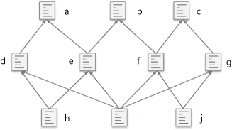
Figure 1: A reference graph.

On the other hand, Co-citation computes the score between $a$ and $c$ as 0 and the score between $d$ and $g$ as 1. A closer look reveals that $d$ references $a$ and that $g$ references $c$. Since the papers with the similarity score of 1 ($d$ and $g$) reference them, $a$ and $c$ may be regarded somewhat similar. SimRank captures this intuition such that the objects referenced by similar objects are similar. That is, SimRank computes the similarity score recursively. Equation 4 represents SimRank. In Equation 4, $R_{k}(p,q)$ denotes the similarity score between $p$ and $q$ at iteration $k$ , and $I_{i}(p)$ denotes the paper connected to $p$ through $i$-th in-link. $C$ is a decay factor for attenuating the similarity score during similarity propagation, where $C\in[0,1]$.

$$R_{0}(p,q)=\left\{\begin{array}[]{ll}0&\textrm{if $p\neq q$}\\ 1&\textrm{if $p=q$}\end{array},\right.$$ (6)

$$R_{k+1}(p,q)=\frac{C}{|I(p)||I(q)|}\sum_{i=1}^{|I(p)|}\sum_{j=1}^{|I(q)|}R_{k}(I_{i}(p),I_{j}(q))$$

By using globalized neighbors, SimRank improves the accuracy of Co-citation which uses localized neighbors only. Similarly, rvs-SimRank and P-Rank improve Coupling and Amsler, respectively. Equation 5 represents rvs-SimRank. The only difference between rvs-SimRank and SimRank is the type of links used. Equation 6 represents P-Rank. As shown in Equation 6, P-Rank measures the similarity score between two objects as a weighted sum of the similarity scores by rvs-SimRank and SimRank.

$$R_{0}(p,q)=\left\{\begin{array}[]{ll}0&\textrm{if $p\neq q$}\\ 1&\textrm{if $p=q$}\end{array},\right.$$ (10)

$$R_{k+1}(p,q)=\frac{C}{|O(p)||O(q)|}\sum_{i=1}^{|O(p)|}\sum_{j=1}^{|O(q)|}R_{k}(O_{i}(p),O_{j}(q))$$

$$R_{0}(p,q)=\left\{\begin{array}[]{ll}0&\textrm{if $p\neq q$}\\ 1&\textrm{if $p=q$}\end{array},\right.$$ (14)

$$R_{k+1}(p,q)=\lambda\times\frac{C}{|I(p)||I(q)|}\sum_{i=1}^{|I(p)|}\sum_{j=1}^{|I(q)|}R_{k}(I_{i}(p),I_{j}(q))$$

$$+(1-\lambda)\times\frac{C}{|O(p)||O(q)|}\sum_{i=1}^{|O(p)|}\sum_{j=1}^{|O(q)|}R_{k}(O_{i}(p),O_{j}(q))$$ (15)

Table 1 summarizes the existing similarity measures [5]. When $k=1$, $C=1$, and $\lambda=1$ (or $\lambda=0$), Equation 6 represents Co-citation (or Coupling). When $k=1$, $C=1$ and $\lambda=0.5$, Equation 6 represents Amsler. When $k=\infty$, Equation 6 represents SimRank, rvs-SimRank, and P-Rank depending on the value of $\lambda$. Even though $k=\infty$ for SimRank, rvs-SimRank, and P-Rank, empirically the similarity scores by SimRank, rvs-SimRank, and P-Rank tend to converge at $k=4$ or $5$ [5][8].

Table 1: Relationship among similarity measures (Adopted from [5])

Links used k	In-link	Out-link	Both
k=1	Co-citation	Coupling	Amsler
	C=1, $\lambda$=1	C=1, $\lambda$=0	C=1, $\lambda$=1/2
k=$\infty$	SimRank	rvs-SimRank	P-Rank
	C=varies, $\lambda$=1	C=varies, $\lambda$=0	C, $\lambda$=varies

2.2 Problems with Existing Similarity Measures

Scientific literature databases have two characteristics that are different from general databases. First, very old papers are often not in the database. Second, there exist few papers that reference recently-published papers. Due to these two characteristics, all existing similarity measures fail to compute the similarity score correctly in scientific literature databases, at least in one of the following three cases.

(P1)	measuring the similarity between old, but similar papers
(P2)	measuring the similarity between recent, but similar papers
(P3)	measuring the similarity between two similar papers: one old, the other recent

Figure 2 represents the reference relations among papers as a graph. In Figure 2, $a$ to $l$ represent papers, and arrows represent the reference relations between papers. The papers on top of the figure are older, and the papers at bottom are more recent. An example of (P1) happens when the similarity score between $a$ and $b$ is computed. The similarity score computed by Coupling (rvs-SimRank) is 0 (near 0) because these papers have no out-links. The similarity score by Amsler (P-Rank) is not 0, because the score by Co-citation is 1. The maximum score by Amsler (P-Rank), however, would be at most 0.5 (assuming the relative weight for Coupling and Co-citation is 0.5). That is, the score by Amsler (P-Rank) is inaccurate. An example of (P2) happens when the score between $k$ and $l$ is computed. The score computed by Co-citation (SimRank) is 0 (near 0) because these papers have no in-links. The score by Amsler (P-Rank) would be 0.5 (near 0.5), even though they have a common out-link neighbor $i$. An example of (P3) happens when the score between $e$ and $l$ is computed. The score computed by all existing similarity measures is 0 or near 0.

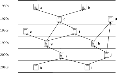
Figure 2: A graph of the reference relationships with publishing dates.

Coupling, Co-citation, and Amsler fail to capture the similarity between papers in scientific literature databases. Rvs-SimRank, SimRank, and P-Rank are plagued with the same problems, since they are the iterative extensions of Coupling, Co-citation, and Amsler, respectively.

3 Proposed Similarity Measure

In this section, we propose a new similarity measure called C-Rank and describe its algorithm in detail. We also discuss a normalization method appropriate for the new measure.

3.1 Main Idea

Two papers $p$ and $q$ should receive a high similarity score in the following three cases.

(C1)	the number of papers referenced by both $p$ and $q$ is high
(C2)	the number of papers which reference both $p$ and $q$ is high
(C3)	the number of the papers which are referenced by $p$ reference $q$ is high

We define the paper which is referenced by both papers as OP (common Out-link Paper), paper which references both papers as IP (common In-link Paper), and paper which is referenced by the one paper and references the other as BP (common Between Paper). In Figure 2, for example, $f$ is an OP of $g$ and $h$, $h$ is an IP of $d$ and $f$, and $c$ is a BP of $a$ and $f$.

The existing measures can be used in (C1) and (C2) cases. Co-citation or SimRank can be used for (C1), and Coupling or rvs-SimRank can be used for (C2). In Figure 2, for example, Co-citation (SimRank) can be used to measure the similarity between $g$ and $h$, and Coupling (rvs-SimRank) can be used to measure the similarity between d and $f$. The existing measures, however, cannot correctly measure the similarity in (C3). In Figure 2, for example, existing measures fail to compute the similarity between $a$ and $f$. A similarity measure that counts BPs should be suitable for this case. Of course, a BP-based similarity measure cannot be used for the papers with publication dates close to each other, such as $g$ and $h$, since there exist few BPs between the papers under consideration.

To compute the score correctly in all three cases, therefore, we propose to use all three measures, Co-citation (or SimRank), Coupling (or rvs-SimRank), and a new BP-based measure. When combining all three measures, a weighted sum of similarity scores from the three measures could have been used, similar to Amsler (or P-Rank). Note that this would suffer the same problem faced by Amsler (or P-Rank) that one of the scores may be near 0, which results in the score that is much lower than the correct value. Instead of using a weighted sum, therefore, we propose a new measure that considers three cases simultaneously.

3.2 C-Rank

Though papers are classified into OPs, IPs, and BPs based on the direction of links, their role is the same: they are used to compute the similarity between two papers. So, we disregard the direction of links, which results in a single type of links that connect two papers. We define the papers which connect two papers as $Connectors$. When disregarding the direction of references, Coupling (or rvs-SimRank), Co-citation (or SimRank), and a BP-based similarity measure are unified as a single measure that computes the similarity score based on the number of Connectors in an undirected graph.

We propose a Connector-based similarity measure called C-Rank. C-Rank uses both in-links and out-links at the same time. Equation 7 represents C-Rank, where $L(p)$ denotes the set of undirected link neighbors of paper $p$. Similar to that the accuracy of Co-citation (Coupling) is improved by iterative SimRank (rvs-SimRank), C-Rank is defined iteratively.

$$R_{0}(p,q)=\left\{\begin{array}[]{ll}0&\textrm{if $p\neq q$}\\ 1&\textrm{if $p=q$}\end{array},\right.$$ (18)

$$R_{k+1}(p,q)=\frac{C}{|L(p)||L(q)|}\sum_{i=1}^{|L(p)|}\sum_{j=1}^{|L(q)|}R_{k}(L_{i}(p),L_{j}(q))$$ (19)

Unlike Amsler or P-Rank, C-Rank does not need parameter $\lambda$, because C-Rank unifies in-links and out-links into undirected links. Furthermore, C-Rank has the effect similar to increasing the weight of Co-citation (SimRank) when computing the score between old papers, increasing the weight of Coupling (rvs-SimRank) when computing the score between recent papers, and increasing the weight of a BP-based similarity measure when computing the score between old and recent papers. The user does not have to set the value of $\lambda$ when using C-Rank. In experiments, we show that the accuracy of C-Rank is higher than those of Amsler (P-Rank) with different $\lambda$ values.

One of the evaluation criteria for link-based similarity measures is how many pairs of objects can be measured [5]. SimRank fails to compute the similarity when a paper has no in-link, and rvs-SimRank fails when a paper has no out-link. Although being able to compute the similarity scores for more pairs than any other measures, P-Rank measures similarity for less number of pairs than C-Rank. This is because P-Rank fails to compute the similarity between an old paper and a recent one. In experiments, we show that the number of pairs of papers computed by C-Rank is more than that of any other measures.

Treating both in-links and out-links as undirected might be thought to result in loss of semantics of the direction of links. By disregarding the direction of links, however, C-Rank is able to consider all three cases mentioned in 2.2. Thus, the measure has more advantages than disadvantages when computing the similarities among papers.

3.3 Normalization

In previous studies, two types of normalization methods are used to prevent a problem that the similarity score between two papers increases as the number of links increases. Used in Coupling (or Co-citation), Jaccard coefficient normalizes the similarity score by dividing the number of papers which are referenced by (or reference) both papers by the sum of the number of the papers each paper references (or is referenced by) [14]. Rvs-SimRank, SimRank, and P-Rank have used the pairwise normalization method. SimRank, for example, builds a set of pairs between the papers that reference any one of the two papers under consideration, computes the sum of similarity scores of all pairs, and divides it by the product of the number of in-links to each paper.

In scientific literature databases, some well-known papers are referenced by the many other papers, and people who use retrieval services would be interested in those quality papers. Since the pairwise normalization method lowers the similarity score of the papers with many in-links, the similarity scores between two famous papers can be very low [11]. Figure 3 represents an example of the problem with the pairwise normalization method. In Figure 3, papers $p$ and $q$ are referenced by all the other papers, and should be determined similar. When the number of papers which reference both $p$ and $q$ is $k$, however, the similarity score with pairwise normalization becomes $\frac{1}{k}$. The same problem exists when the similarity is computed iteratively, although the score may be somewhat higher than $\frac{1}{k}$ [11]. So, for the scientific literature databases where famous papers (in which users would be interested) have many in-links, Jaccard coefficient seems a better normalization method. Equation 8 represents C-Rank with Jaccard coefficient. In Equation 8, ‘$\setminus$’ denotes different set. In experiments, we show Jaccard coefficient is more suitable than pairwise normalization for scientific literature databases.

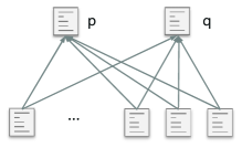
Figure 3: An example showing the problem with the pairwise normalization method.

3.4 Recursive C-Rank

The recursive C-Rank in Equation (8) has the following four properties. For any papers $p$ and $q$, the iterative C-Rank of $p$ and $q$ is the same as that of $q$ and $p$ (symmetry). The iterative C-Rank is non-decreasing during similarity computation (monotonicity). Existence and uniqueness guarantee that there exists a unique solution to iterative C-Rank which reaches a fixed point by iterative computation. The prove can be found in Appendix.

(Symmetry)	$R_{k}(p,q)=R_{k}(q,p)$
(Monotonicity)	$0\leq R_{k}(p,q)\leq R_{k+1}(p,q)\leq 1$
(Existence)	The solution to the iterative C-Rank equations always exists and converges to a fixed point, $s(*,*)$, which is the theoretical solution to the recursive C-Rank equations.
(Uniqueness)	The solution to the iterative C-Rank equation is unique when $C\neq 1$.

$$R_{0}(p,q) =\left\{\begin{array}[]{ll}0&\textrm{if $p\neq q$}\\ 1&\textrm{if $p=q$}\end{array},\right.$$ (22)

$$R_{k+1}(p,q) =C\times(\frac{|L(p)\cap L(q)|}{|L(p)\cup L(q)|}\times 1$$

$$+\frac{1}{|L(p)\cup L(q)||L(q)|}\times\sum_{p^{\prime}\in L(p)\setminus L(q)}\sum_{q^{\prime}\in L(q)}R_{k}(p^{\prime},q^{\prime})$$

$$+\frac{1}{|L(p)\cup L(q)||L(p)|}\times\sum_{p^{\prime}\in L(p)}\sum_{q^{\prime}\in L(q)\setminus L(p)}R_{k}(p^{\prime},q^{\prime})$$

(23)

3.5 Algorithm

Table 2 shows the algorithm of C-Rank. For every pair of papers $(p,q)$, an entry $R(p,q)$ maintains the intermediate C-Rank score of (a,b) during iterative computation. Because the $k$-th iterative C-Rank score is computed based on C-Rank scores in the $(k-1)-$th iteration, an auxiliary similarity score store $R*(p,q)$ is maintained accordingly. The code first initializes $R_{0}(p,q)$ based on Table 2 (Lines 1$\sim$4). During iterative computation, $R*(*,*)$, is updated by $R(*,*)$ in the $k-1$ iteration, based on Table 2 (Lines 6$\sim$17). Then $R_{k}(*,*)$ is substituted by $R_{k+1}(*,*)$ for further iteration (Lines 18$\sim$20). This iterative procedure is repeated $k$ times (Lines 5$\sim$21).

The space complexity of all existing measures are $O(n^{2})$ because the measures must store pairs of all papers. Let $d^{1}$ and $d^{2}$ be the average number of in-links and out-links of all papers, respectively, the time complexity of rvs-SimRank, SimRank, and P-Rank are $O(k\cdot d_{1}^{2}\cdot n^{2})$, $O(k\cdot d_{2}^{2}\cdot n^{2})$, and $O(k\cdot(d_{1}^{2}+d_{2}^{2})\cdot n^{2})$), respectively [5]. The time complexity of C-Rank is $O(k\cdot(d_{1}+d_{2})^{2}\cdot n^{2})$, which is slightly higher than the others. However, the worst case time complexity of all existing iterative measures including C-Rank is $O(n^{4})$.

The time complexity of C-Rank may become too high. There have been many methods to improve the time complexity of SimRank [5][8][11][12][13][18]. These methods can be applied to C-Rank, because the equation of C-Rank and that of SimRank are similar.

4 Experiments

In this section, we compare the effectiveness of C-Rank and the existing similarity measures.

4.1 Experimental Setup

Our experiments ran on a scientific literature database with papers from DBLP and reference information crawled from Libra. We used the papers related to the database research because the running time of the existing similarity measures and C-Rank in the large database can become very high. We used the publication venues listed in [19] to select papers related to database research. Table 3 lists the publication venues in [19]. The number of papers was 23,795 and the number of references (to the papers in the dataset) was 126,281. All our experiments were performed on an Intel PC with Quad Core 2.67GHz CPU, running Windows 2008. We compared C-Rank with rvs-SimRank, SimRank, and P-Rank, because Coupling, Co-citation, and Amsler could be expressed using rvs-SimRank, SimRank, and P-Rank, respectively. For fairness of comparison, we set the decay factor $C=0.8$ for all measures and the relative weight $\lambda$ to be 0.5 for P-Rank, unless otherwise noted. All the default values of parameters are set in accordance with [5].

Table 2: The C-Rank Algorithm

	C-Rank ($G$, $C$, $k$)
	Input: A reference graph $G$ (an undirected graph),
	the decay factor $C$, the iteration number $k$
	Output: C-Rank score $R(*,*)$
1	foreach $p\in G$ do /* Initialization */
2	foreach $q\in G$ do
3	if $p==q$ then $R(p,q)=1$
4	else $R(p,q)=0$
5	while ($n<k$) do /* Iteration */
6	foreach $p\in G$ do
7	foreach $q\in G$ do
8	$R*(p,q)=\frac{|L(p)\cap L(q)|}{|L(p)\cup L(q)|}$
9	foreach $l_{p}\in L(p)\backslash L(q)$
10	foreach $l_{q}\in L(q)$
11	differentSetofp += $R(l_{p},l_{q})$
12	differentSetofp $\times$= $\frac{1}{|L(p)\cup L(q)||L(q)|}$
13	foreach $l_{p}\in L(q)\backslash L(p)$
14	foreach $l_{q}\in L(p)$
15	differentSetofq += $R(l_{p},l_{q})$
16	differentSetofq $\times$= $\frac{1}{|L(p)\cup L(q)||L(p)|}$
17	$R*(p,q)+=C\times$ (differentSetofp + differentSetofq)
18	foreach $p\in G$ do /* Update */
19	foreach $q\in G$ do
20	$R(p,q)=R*(p,q)$
21	$n=n+1$
22	return R(*,*)

4.2 Accurate Evaluation Method

Previous studies on similarity measures used various evaluation methods. [2] and [3] evaluated Coupling and Co-citation qualitatively, showing some example cases. Although easy to use, however, qualitative evaluations do not provide any concrete evidence on which measure is better or how accurate each measure is. [8] used a text-based similarity measure and Co-citation as ground truth to evaluate the accuracy of SimRank. Because the text-based similarity measure is less accurate than SimRank, and Co-citation does not generate similarity scores accurately at least in scientific literature databases, using these two measures as ground truth do not seem a good evaluation method for scientific literature databases. [5] clustered papers using the similarity score by SimRank and the similarity score by P-Rank, respectively, and evaluated the accuracy of two measures by comparing the similarity scores of papers from the same cluster and those from different clusters. Although used for evaluating the quality of clustering in clustering research, this method is not suitable for evaluating the similarity measure because the results are dependent on the type of data and clustering algorithm [20].

Table 3: Publication venues related to database research [19]

ADBIS, ADC, ARTDB, BNCOD, CDB, CIKM, CoopIS, DANTE, DASFAA, DAWAK, DB, DBPL, DBSEC, DEXA, DKD, DKE, DL, DMKD, DNIS, DOLAP, DOOD, DPD, DPDS, DS, EDBT, ER, FODO, FOIKS, FQAS, GIS, HPTS, ICDE, ICDM, ICDT, ICIS, IDA, IDEAL, IDEAS, IGSI, Inf. Process, Lett., Inf. Sci., Inf. Syst., IPM, IQIS, ISF, ISR, IW-MMDBMS, IWDM, JDM, JIIS, JMIS, K-CAPKA, KDD, KER, KIS, KR, MDA, MFDBS, MLDM, MMDB, MSS, NLDB, OODBS, PAKDD, PKDD, PODS, RIDE, RIDS, SIGKDD Exp., SIGMOD, SIGMOD Rec., SSD, SSDMB, TKDE, TODS, TOIS, TSDM, UIDIS, VDB, VLDB, VLDB-J, WebDB, WIDM, WISE, XMLEC

One of the most accurate ways to evaluate the accuracy of a similarity measure would be to ask humans [8], but user studies are expensive and time consuming. We propose a new evaluation method that achieves similar effects without employing user studies. We ask domain experts to select the papers similar to each other, and evaluate each similarity measure based on the similarity score between the selected papers. The higher the score is, the more accurate the similarity measure is.

The evaluation process in detail is as follows. First, we select five well-known fields in data mining (clustering, sequential pattern mining, graph mining, spatial databases, link mining) and select the references at the end of each chapter for each field from a data mining text book [14]. The references include both old and recent papers. Second, we use one of the references to be a query paper and find the $m$ highest scoring papers (where $m$ can be 10, 20, 30, 40, and 50) by each similarity measure. Third, we compute the precision of each similarity measure by comparing the m highest scoring papers to those in the reference list of the field of the query paper. Fourth, we repeat the second and third steps until all references are used as a query paper.

4.3 Experimental Results

4.3.1 Normalization Method

In this section, we compare the accuracy of similarity measures with Jaccard coefficient and that with the pairwise normalization method. Figure 4 shows the accuracy of P-Rank and C-Rank with different normalization methods. (The other measures, rvs-SimRank and SimRank, exhibit similar results, and thus omitted.) The accuracy of both similarity measures with Jaccard coefficient is higher than that with pairwise normalization. The results confirm that Jaccard coefficient is a more suitable normalization method for scientific literature databases. Note that the accuracy of C-Rank with pairwise normalization is lower than that of P-Rank with pairwise normalization. This is because C-Rank uses more links than P-Rank as mentioned 3.3.

4.3.2 Top 10 Rankings

In this section, we confirm that C-Rank measures similarity properly by extracting the top 10 highest-scoring papers by C-Rank when paired with a well-known paper as a query paper. We use [21] and [22], two well-known papers in the database and data mining research field, respectively. Table 4 lists top 10 highest-scoring papers when paired with [21], and Table 5 lists the top 10 highest-scoring papers when paired with [22]. [21] proposed R-Tree as a multidimensional index. In Table 4, the highest-scoring papers by C-Rank are mostly related to multidimensional indexes. [22] proposed BIRCH as a clustering method. In Table 5, the papers by C-Rank are mostly related to clustering. The results show that C-Rank can provide a set of papers similar to the paper under consideration.

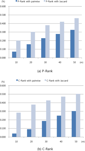
Figure 4: Comparing Jaccard coefficient and pairwise normalization method.

4.3.3 Failure of Existing Similarity Measures

In this section, we demonstrate the problem of existing similarity measures when applied to scientific literature databases using three cases identified in Section 2.2. We also show that C-Rank computes the similarity score properly in all three cases. For demonstration purposes, we select [23], [24] and [21], [25] as the pairs of old papers but similar papers, [26], [27] and [28], [29] as the pairs of recent papers but similar papers, and [25], [30] and [31], [32] as the pairs of an old and a recent paper.

Table 6 shows the result of case analysis. Six cases are illustrated in Table 6, but all other examples tested show similar results. In Table 6, the similarity scores between old but similar papers by rvs-SimRank are 0 in both cases. As noted in Section II.B, rvs-SimRank identifies incorrectly that the papers are not similar because they have no common out-links. Similarly, the similarity scores between recent but similar papers by SimRank are 0 in both cases. SimRank identifies incorrectly that the papers are not similar because they have no common in-links. Furthermore, all existing similarity measures compute the similarity scores between the papers with different publication dates as 0. C-Rank is the only one that measures the similarity of those papers. That is, C-Rank is able to capture the similarity between the papers with different publishing dates. Note that the scores by C-Rank are not high in both cases. This is because the problem tackled in the old paper and that in the newer paper, although somewhat similar, have become less in common as time passes on. The original problem may have changed to a more specific problem, or it may have changed to solve more general problem, etc.

Table 4: Top 10 papers similar to [21]

1	The R*-Tree: An Efficient and Robust Access Method …
2	The R+-Tree: A Dynamic Index for Multi-Dimensional …
3	Nearest Neighbor Queries
4	The K-D-B-Tree: A Search Structure For Large …
5	The X-tree : An Index Structure or …
6	On Packing R-trees
7	The Grid File: An Adaptable, Symmetric Multikey …
8	Efficient Processing of Spatial Joins Using R-Trees
9	Hilbert R-tree: An Improved R-tree using Fractals
10	The SR-tree: An Index Structure for High-Dimensional …

Table 5: Top 10 papers similar to [22]

1	Efficient and Effective Clustering Methods …
2	CURE: An Efficient Clustering Algorithm …
3	A Density-Based Algorithm for Discovering Clusters …
4	Automatic Subspace Clustering of High Dimensional …
5	Scaling Clustering Algorithms to Large Databases
6	WaveCluster: A Multi-Resolution Clustering Approach …
7	Fast Algorithms for Projected Clustering
8	STING: A Statistical Information Grid Approach …
9	An Efficient Approach to Clustering in Large …
10	OPTICS: Ordering Points To Identify the Clustering…

Table 6: The results of case analysis

	old papers	recent papers	an old
			and a recent paper
	[23] and [24]	[26] and [27]	[25] and [30]
	[21] and [25]	[28] and [29]	[31] and [32]
rvs-SimRank	0	0.278	0
	0	0.189	0
SimRank	0.179	0	0
	0.141	0	0
P-Rank	0.114	0.198	0
	0.082	0.096	0
C-Rank	0.240	0.282	0.050
	0.175	0.210	0.047

4.3.4 Accuracy of Similarity Measures

Figure 5 represents the accuracy of different similarity measures. In Figure 5, x-axis represents the number of top $m$ scoring papers, and y-axis represents the accuracy of each similarity measure. As shown in Figure 5, the accuracy of C-Rank is higher than the other similarity measures regardless of the value of $m$. The results indicate that C-Rank is more accurate than the other measures in scientific literature databases.

4.3.5 Distribution of Similarity Scores

In this section, we count the number of pairs whose similarity is computable by each similarity measure. Figure 6 shows the distribution of the similarity scores by each similarity measure. In Figure 6, x-axis represents the range of similarity scores, where [$lb$, $ub$) indicates $lb$ is included and $ub$ is not included in the range, and y-axis represents the number of pairs of papers. In Figure 6, y-axis is in log scale, because for most pairs, the similarity scores are either in N/A or in [0, 0.1). N/A represents the pairs whose similarity cannot be measured. As shown in Figure 6, there are no such pairs of papers whose similarity scores are N/A by C-Rank. This implies that C-Rank computes the similarity score between all pairs of papers because C-Rank uses both in-link and out-link simultaneously. In Figure 6, the pairs of papers whose similarity scores are N/A by the other measures can be thought to be computed as near 0 by C-Rank. However, we note that the number of pairs in [0, 0.1) by C-Rank is not too much different from those of other measures. This result indicates that C-Rank provides meaningful similarity scores for the pairs of papers even when their computation is infeasible with the other similarity measures.

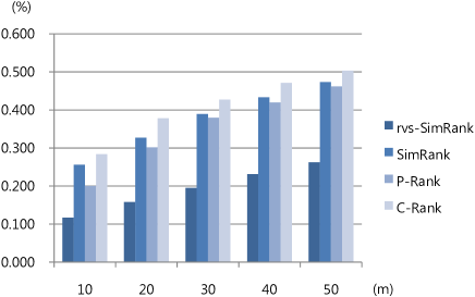
Figure 5: The accuracy of the similarity measures.

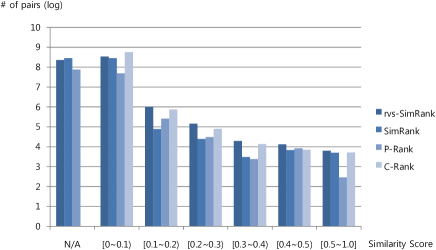
Figure 6: Distributions of the similarity scores.

4.3.6 Similarity Scores with Variations of the Number of Iterations

In this section, we examine the algorithmic nature of similarity measures by tracing the changes in the similarity score while varying $k$. Figure 7 represents the average of the similarity scores of the 10 highest-scoring pairs of papers while varying $k$ from 1 to 10. In Figure 7, x-axis represents the number of iterations, and y-axis represents the average of the scores of the top 10 highest-scoring pairs of papers by rvs-SimRank, SimRank, P-Rank, and C-Rank, respectively. The similarity score $R_{k}(*,*)$ becomes more accurate on successive iterations. Iteration 2, which computes $R_{2}(*,*)$ from $R_{1}(*,*)$, can be thought of as the first iteration taking advantage of the recursive power of algorithms for similarity computation. Subsequent changes become increasingly minor, suggesting a rapid convergence. The score by SimRank converges at $k=3$, the score by rvs-SimRank converges at $k=5$, the score by P-Rank converges at $k=6$, and the score by C-Rank converges at $k=9$. Because it utilizes the highest number of links, C-Rank is the last one to converge.

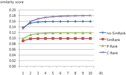
Figure 7: The similarity scores with different $k$ values.

4.3.7 Similarity Scores with Variations of Decay Factor

In this section, we show how the decay factor $C$ is related to the speed of convergence in C-Rank. Figure 8 represents the average similarity scores by C-Rank with variations of $C$. In Figure 8, x-axis represents the number of iterations, and y-axis represents the average similarity score by the top 10 highest-scoring pairs of papers. The decay factor, $C$, is set to be 0.2, 0.5, and 0.8, respectively. It is obvious that the similarity score of C-Rank increases with the increase of $C$. When $C=0.2$, C-Rank converges fast at $k=2$. When $C=0.8$, on the other hand, C-Rank converges at the $9$-th iteration. When $C$ is low, the recursive power of C-Rank is weakened such that only the papers in local or near-local neighborhood are used in similarity computation. When $C$ is high, more papers in a more global neighborhood can be used in computing the similarity recursively. When $C$ is high, therefore, the convergence takes more time.

4.3.8 Accuracy of Similarity Measures with Variations of the Relative Weight

So far, we have used the relative weight to be 0.5 in P-Rank. In this section, we compare the accuracy of C-Rank and those of P-Rank with variations of $\lambda$. The $\lambda$ is set to be 0.3, 0.5, and 0.8. Figure 9 represents the accuracy of C-Rank and P-Rank with variations of $\lambda$. In Figure 9, x-axis represents the number of the top $m$ scoring papers, and y-axis represents the accuracy of each similarity measure. The accuracy of C-Rank is higher than those of P-Rank regardless of the value of $\lambda$ in most cases. Although the accuracy of P-Rank with $\lambda=0.8$ is higher than that of C-Rank in two cases, when $m=40$ and $m=50$, the similarity score is more important when $m$ is low, especially in scientific literature retrieval services, and C-Rank achieves a higher accuracy than P-Rank when $m$ is 10, 20, and 30.

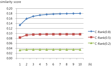
Figure 8: The similarity scores with different $C$ values.

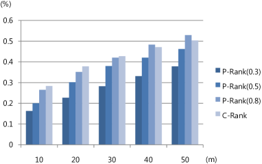
Figure 9: The accuracy of C-Rank and P-Rank with different $\lambda$ values.

5 Conclusions

In this paper, we propose C-Rank, a new similarity measure for scientific literature databases. We examine two notable characteristics in scientific literature databases and identify three cases where all existing similarity measures fail to compute the similarity score correctly. Our observations lead to the development of C-Rank, which uses both in-link and out-link while disregarding the direction of references. In addition, we verify Jaccard coefficient is more appropriate for scientific literature databases, and propose an evaluation method for measuring the accuracy of similarity measures. For experiments, we have built a database with real papers from DBLP and reference information crawled from Libra. Experimental results show that C-Rank achieves a higher effectiveness than existing similarity measures in most cases.

The contributions of this paper are as follows:

1. We have pointed out that existing similarity measures fail to compute the similarity score properly for scientific papers.

2. We have proposed a new similarity measure for computing the similarity score among papers called C-Rank.

3. We have proposed a normalization method suitable for scientific literature databases.

4. We have proposed a quantitative evaluation method which matches the intuition of users.

6 Appendix

We prove following four mathematical properties:

1.	(Symmetry) According to Equation(8), it is $R_{k}(a,b)=R_{k}(b,a)$ for $k\geq 0$.
2.	(Monotonicity) If $a=b$, $R_{0}(a,b)=R_{1}(a,b)=...=1$, so it is that the monotonicity property holds. We consider $a\neq b$. According to Equation(8), $R_{0}(a,b)=0$. Base on Equation(8), $0\leq$ $R_{1}(a,b)\leq 1$. So, $0\leq R_{0}(a,b)\leq$ $R_{1}(a,b)\leq 1$. We assume that for all $k$, $0\leq R_{k-1}(a,b)\leq R_{k}(a,b)\leq 1$, then
	$R_{k-1}(a,b)-R_{k}(a,b)=C\times$$\frac{|L(a)\setminus L(b)|}{|L(a)\cup L(b)|}\times$$\frac{1}{|L(a)\setminus L(b)||L(b)|}$
	$\times\sum\limits_{a^{\prime}\in L(a)\setminus L(b)}\sum\limits_{b^{\prime}\in L(b)}[R_{k}(a^{\prime},b^{\prime})-R_{k-1}(a^{\prime},b^{\prime})]$
	$+C\times\frac{|L(b)\setminus L(a)|}{|L(a)\cup L(b)|}\times\frac{1}{|L(b)\setminus L(a)||L(a)|}$
	$\times\sum\limits_{a^{\prime}\in L(a)}\sum\limits_{b^{\prime}\in L(b)\setminus L(a)}[R_{k}(a^{\prime},b^{\prime})-R_{k-1}(a^{\prime},b^{\prime})]$
	Based on the assumption, we have $(R_{k}(a,b)-R_{k-1}(a,b))\geq 0$, $\forall a,b\in G$, so the left hand side $R_{k+1}(a,b)-R_{k}(a,b)\geq 0$ holds. By induction, we draw the conclusion that for any $k$, $R_{k}\leq R_{k+1}$. And based on the assumption, $0\leq R_{k}(a,b)\leq 1$, so
	1) $C\times\frac{|L(a)\cap L(b)|}{|L(p)\cup I(a)|}\times 1$
	2) $C\times$$\frac{|L(a)\setminus L(b)|}{|L(a)\cup L(b)|}\times$$\frac{1}{|L(a)\setminus L(b)||L(b)|}$
	$\times\sum\limits_{a^{\prime}\in L(a)\setminus L(b)}\sum\limits_{b^{\prime}\in L(b)}R_{k}(a^{\prime},b^{\prime})$
	$\leq C\times\frac{|L(a)\setminus L(b)|}{|L(a)\cup L(b)|}\times\frac{1}{|L(a)\setminus L(b)||L(b)|}$
	$\times\sum\limits_{a^{\prime}\in L(a)\setminus L(b)}\sum\limits_{b^{\prime}\in L(b)}1=C\times\frac{|L(a)\setminus L(b)|}{|L(a)\cup L(b)|}$
	3) $C\times$$\frac{|L(b)\setminus L(a)|}{|L(a)\cup L(b)|}\times$$\frac{1}{|L(b)\setminus L(a)||L(a)|}$
	$\times\sum\limits_{a^{\prime}\in L(a)}\sum\limits_{b^{\prime}\in L(b)\setminus L(a)}R_{k}(a^{\prime},b^{\prime})$
	$\leq C\times\frac{|L(b)\setminus L(a)|}{|L(a)\cup L(b)|}\times\frac{1}{|L(b)\setminus L(a)||L(a)|}$
	$\times\sum\limits_{a^{\prime}\in L(a)}\sum\limits_{b^{\prime}\in L(b)\setminus L(a)}1$
	$=C\times\frac{|L(b)\setminus L(a)|}{|L(a)\cup L(b)|}$
	The above equation represents following
	$C[\frac{|L(a)\cap L(b)|}{|L(p)\cup I(a)|}+\frac{|L(a)\setminus L(b)|}{|L(a)\cup L(b)|}+\frac{|L(b)\setminus L(a)|}{|L(a)\cup L(b)|}]=C$
	so, $R_{k+1}(a,b)\leq C\leq 1$. By induction, we know that for any $k$, $0\leq R_{k}(a,b)\leq 1$.
3.	(Existence) According to (Monotonicity), $\forall a,b\in G$, $R_{k}(a,b)$ is bounded and nondecreasing as $k$ increase. By the Completeness Axiom of calculus, each sequence $R_{k}(a,b)$ converges to a limit $R(a,b)\in[0,1]$. Note $\lim_{k\rightarrow\infty}R_{k}(a,b)=\lim_{k\rightarrow\infty}R_{k+1}(a,b)=R(a,b)$, So we have
	$R(a,b)=\lim\limits_{k\to\infty}R_{k+1}(a,b)$
	$=\lim\limits_{k\to\infty}C\times[\frac{{|L(a)\cap L(b)|}}{{|L(a)\cup L(b)|}}\times 1+\frac{{|L(a)\setminus L(b)|}}{{|L(a)\cup L(b)|}}$
	$\times\frac{1}{{|L(a)\setminus L(b)||L(b)|}}\sum\limits_{a^{\prime}\in L(a)\setminus L(b)}{\sum\limits_{b^{\prime}\in L(b)}{{R_{k}}(a^{\prime},b^{\prime})}}$
	$+\frac{{|L(a)\setminus L(b)|}}{{|L(b)\cup L(a)|}}\times\frac{1}{{|L(b)\setminus L(a)||L(a)|}}\sum\limits_{a^{\prime}\in L(a)}$
	$\times{\sum\limits_{b^{\prime}\in L(b)\setminus L(a)}}{{R_{k}}(a^{\prime},b^{\prime})}]$
	$=C\times[\frac{{|L(a)\cap L(b)|}}{{|L(a)\cup L(b)|}}\times 1+\frac{{|L(a)\setminus L(b)|}}{{|L(a)\cup L(b)|}}$
	$\times\frac{1}{{|L(a)\setminus L(b)||L(b)|}}\sum\limits_{a^{\prime}\in L(a)\setminus L(b)}{\sum\limits_{b^{\prime}\in L(b)}{\lim\limits_{k\to\infty}{R_{k}}(a^{\prime},b^{\prime})}}$
	$+\frac{{|L(a)\setminus L(b)|}}{{|L(b)\cup L(a)|}}\times\frac{1}{{|L(b)\setminus L(a)||L(a)|}}$
	$\times\sum\limits_{a^{\prime}\in L(a)}{\sum\limits_{b^{\prime}\in L(b)\setminus L(a)}}{\lim\limits_{k\to\infty}R_{k}(a^{\prime},b^{\prime})}]$
	$=C\times[\frac{{|L(a)\cap L(b)|}}{{|L(a)\cup L(b)|}}\times 1+\frac{{|L(a)\setminus L(b)|}}{{|L(a)\cup L(b)|}}$
	$\times\frac{1}{{|L(a)\setminus L(b)||L(b)|}}\sum\limits_{a^{\prime}\in L(a)\setminus L(b)}{\sum\limits_{b^{\prime}\in L(b)}{R(a^{\prime},b^{\prime})}}$
	$+\frac{{|L(b)\setminus L(a)|}}{{|L(a)\cup L(b)|}}\times\frac{1}{{|L(b)\setminus L(a)||L(a)|}}$
	$\times\sum\limits_{a^{\prime}\in L(a)}{\sum\limits_{b^{\prime}\in L(b)\setminus L(a)}}{R(a^{\prime},b^{\prime})}]$
	Note that the limit of $R_{k}(*,*)$, with respect to $k$, right satisfies the recursive C-Rank equation, shown in Equation(8).
4.	(Uniqueness) Suppose $s_{1}(*,*)$ and $s_{2}(*,*)$ are two solution to the $n^{2}$ iterative C-Rank equations. for any entities $x,y\in G$, let $\delta(x,y)=s_{1}(x,y)-s_{2}(x,y)$ be their difference. Let $M=\max_{x,y}|\delta(x,y)|$ be the maximum absolute value of any difference. We need to show that $M=0$. Let $|\delta(x,y)|=M$ for some $a,b\in G$. It is obvious that $M=0$ if $a=b$. otherwise,
	$\delta(a,b)=s_{1}(a,b)-s_{2}(a,b)$
	$C\times\frac{|L(a)\setminus L(b)|}{L(a)\cup L(b)|}\times\frac{1}{|L(a)\setminus L(b)||L(b)|}$
	${\tiny\times\sum\limits_{a^{\prime}\in L(a)\setminus L(b)}{\sum\limits_{b^{\prime}\in L(b)}}[S_{1}(L(a^{\prime}),L(b^{\prime}))-S_{2}(L(a^{\prime}),L(b^{\prime}))]}$
	$+C\times\frac{|L(b)\setminus L(a)|}{|L(a)\cup L(b)|}\times\frac{1}{|L(b)\setminus L(a)||L(a)|}$
	${\tiny\times\sum\limits_{a^{\prime}\in L(a)}{\sum\limits_{b^{\prime}\in L(b)\setminus L(a)}}[S_{1}(L(a^{\prime}),L(b^{\prime}))-S_{2}(L(a^{\prime}),L(b^{\prime}))]}$
	Thus,
	$M=|\delta(a,b)|=|C\times\frac{|L(a)\setminus L(b)|}{|L(a)\cup L(b)|}$
	$\times\frac{1}{|L(a)\setminus L(b)||L(b)|}\sum\limits_{a^{\prime}\in L(a)\setminus L(b)}{\sum\limits_{b^{\prime}\in L(b)}{\delta(a^{\prime},b^{\prime})}}$
	$+C\times\frac{|L(b)\setminus L(a)|}{|L(a)\cup L(b)|}\times\frac{1}{|L(b)\setminus L(a)||L(a)|}$
	$\sum\limits_{a^{\prime}\in L(a)}{\sum\limits_{b^{\prime}\in L(b)\setminus L(a)}{\delta(a^{\prime},b^{\prime})}}|$
	$\leq|C\times\frac{|L(a)\setminus L(b)|}{|L(a)\cup L(b)|}\times\frac{1}{|L(a)\setminus L(b)||L(b)|}$
	$\times\sum\limits_{a^{\prime}\in L(a)\setminus L(b)}{\sum\limits_{b^{\prime}\in L(b)}{\delta(a^{\prime},b^{\prime})}}|$
	$+|C\times\frac{|L(b)\setminus L(a)|}{|L(a)\cup L(b)|}\times\frac{1}{|L(b)\setminus L(a)||L(a)|}$
	$\times\sum\limits_{a^{\prime}\in L(a)}{\sum\limits_{b^{\prime}\in L(b)\setminus L(a)}{\delta(a^{\prime},b^{\prime})}}|$
	$\leq C\times\frac{|L(a)\setminus L(b)|}{|L(a)\cup L(b)|}\times\frac{1}{|L(a)\setminus L(b)||L(b)|}$
	$\times\sum\limits_{a^{\prime}\in L(a)\setminus L(b)}{\sum\limits_{b`\in L(b)}{|\delta(a^{\prime},b^{\prime})|}}$
	$+C\times\frac{|L(b)\setminus L(a)|}{|L(a)\cup L(b)|}\times\frac{1}{|L(b)\setminus L(a)||L(a)|}\sum\limits_{a^{\prime}\in L(a)}{\sum\limits_{b^{\prime}\in L(b)\setminus L(a)}{|\delta(a^{\prime},b^{\prime})|}}$
	$\leq C\times\frac{|L(a)\setminus L(b)|}{|L(a)\cup L(b)|}$
	$\times\frac{1}{|L(a)\setminus L(b)||L(b)|}\sum\limits_{a^{\prime}\in L(a)\setminus L(b)}{\sum\limits_{b`\in L(b)}{M}}$
	$+C\times\frac{|L(b)\setminus L(a)|}{|L(a)\cup L(b)|}$
	$\times\frac{1}{|L(b)\setminus L(a)||L(a)|}\sum\limits_{a^{\prime}\in L(a)}{\sum\limits_{b^{\prime}\in L(b)\setminus L(a)}{M}}$
	$\leq C\times\frac{|L(a)\setminus L(b)|}{|L(a)\cup L(b)|}\times M+C\times\frac{|L(b)\setminus L(a)|}{|L(a)\cup L(b)|}\times M$
	$\leq CM\times[\frac{|L(a)\setminus L(b)|}{|L(a)\cup L(b)|}+\frac{|L(b)\setminus L(a)|}{|L(a)\cup L(b)|}]$
	$\leq CM\qquad($by $\frac{|L(a)\setminus L(b)|}{|L(a)\cup L(b)|}+\frac{|L(b)\setminus L(a)|}{|L(a)\cup L(b)|}\leq 1)$
	So $M=0$ when $C\neq 1$.

References

- [1] R. Baeza-Yates and B. Ribeiro-Neto, Modern Information Retrieval, Addison Wesley, 1999.
- [2] M. Kessler, “Bibliographic Coupling between Scientific Papers," Journal of the American Documentation, Vol. 14, No. 1, pp. 10-25, 1963.
- [3] H. Small, “CoCitation in the Scientific Literature: A New Measure of the Relationship between Two Documents,” Journal of the American Society for Information Science, Vol. 24, No. 4, pp. 265-269, 1973.
- [4] U. Shardanband and P. Maes, “Social Information Filtering: Algorithms for Automating ‘Word of Mouth’,” In proc. of Int’l Conf. on Human Factors in Computing Systems, pp. 210-217, 1995.
- [5] P. Zhao, J. Han, and Y. Sun, “P-Rank: A Comprehensive Structural Similarity Measure over Information Networks,” In proc. of Int’l. Conf. on Information and Knowledge Management, pp. 553-562, 2009.
- [6] A. Maguitman, F. Menczer, F. Erdinc, H. Roinestad, and Vespignani, “Algorithmic Computation and Approximation of Semantic Similarity,” WWW Journal, Vol. 9, pp. 431-456, 2006.
- [7] R. Amsler, “Application of Citation-Based Automatic Classification,” The University of Texas at Austin Linguistics Research Center, Technical Report, 1972.
- [8] G. Jeh and J. Widom, “SimRank: A Measure of Structural-Context Similarity,” In Proc. Int l. Conf. on Special Interest Group on Knowledge Discovery and Data, pp. 538-543, 2002.
- [9] D. Liben-Nowell and J. Kleinberg, “The Link Prediction Problem for Social Networks,” In proc. of Int’l. Conf. on Information and Knowledge Management, pp. 556-559, 2003.
- [10] W. Lu, J. Janssen, E. Milios, and N. Japkowicz, “Node Similarity in Networked Information Spaces,” In Proc. Conf. of the centre for Advanced Studies on Collaborative research, pp. 11, 2001.
- [11] D. Fogaras and B. Rcz, “Scaling Link-based Similarity Search,” In Proc. of Int’l. Conf. on World Wide Web, pp. 641-650, 2005.
- [12] X. Yin, J. Han, and P. S. Yu, “LinkClus: Efficient Clustering via Heterogeneous Semantic Links,” In Proc. of Int’l Conf. on Vary Large Data Bases, pp. 427-438, 2006.
- [13] I. Antonellis, H. Garcia-Molina, and C. Chang, “Simrank++: Query Rewriting through Link Analysis of the Click Graph,” In Proc. of Int’l Conf. on Vary Large Data Bases, pp. 408-421, 2008.
- [14] J. Han and M. Kamber, Data Mining: Concepts and Techniques, 2nd ed., Morgan Kaufmann, 2006.
- [15] R. Larson, “Bibliometrics of the World-Wide Web: An Exploratory Analysis of the Intellectual Structure of Cyberspace,” In Proc. of the Annual Meeting of the American Society for Information Science, 1996.
- [16] J. Pitkow and P. Pirolli, “Life, Death, and Lawfulness on the Electronic Frontier,” In Proc. of Int’l. Conf. on Human Factors in Computing Systems, pp. 383-390, 1997.
- [17] A. Popescul, G. Flake, S. Lawrence, L. Ungar, and C. Giles, “Clustering and Identifying Temporal Trends in Document Databases,” In Proc. of the IEEE Advances in Digital Libraries, pp. 173, 2000.
- [18] D. Lizorkin, P. Velikhov, M. Grinev, and D. Turdakov, “Accuracy Estimate and Optimization Techniques for SimRank Computation,” In Proc. of Vary Large Data Bases Endowment, Vol. 1, 422-433, 2008.
- [19] S. Yan and D. Lee, “Toward Alternative Measures for Ranking Venues: A Case of Database Research Community,” In Proc. Int’l. ACM/IEEE-CS Joint Conf. on Digital Libraries, pp. 235-244, 2007.
- [20] R. Xu and D. Wunsch, “Survey of Clustering Algorithms,” IEEE Transactions on Neural Networks, Vol. 16, No. 3, 2005.
- [21] A. Guttman, “R-Trees: A Dynamic Index Structure for Spatial Searching,” In Proc. of Int’l Conf. on Management of Data, pp. 47-57, 1984.
- [22] T. Zhang, R. Ramakrishnam, and M. Livny, “BIRCH: an Efficient Data Clustering Method for Very Large Databases,” In Proc. Int’l. Conf. on Management of Data, pp. 103-114, 1996.
- [23] G. Knott, “Expandable Open Addressing Hash Table Storage and Retrieval,” In Proc. of ACM SIGFIDET (now SIGMOD) Workshop on Data Description, pp. 187-206, 1971.
- [24] S. Ghosh and V. Lum, “Analysis of Collisions when Hashing by Division,” Information Systems, Vol. 1, pp. 15-22, 1975.
- [25] J. Robinson, “The K-D-B-Tree: A Search Structure for Large Multidimensional Dynamic Indexes,” In Proc. of Int’l. Conf. on Management of Data, pp. 10-18, 1981.
- [26] C. Wang, W. Wang, J. Pei, Y. Zhu, B. Shi, “Scalable Mining of Large Disk-based Graph Databases,” In Proc. of Int’l. Conf. on Knowledge Discovery and Data mining, pp. 316-325, 2004.
- [27] S. Nijssen, J. Kok, “A Quickstart in Frequent Structure Mining Can Make a Difference,” In Proc. of Int’l. Conf. on Knowledge Discovery and Data mining, pp. 647-652, 2004.
- [28] S. Cong, J. Han, and D. Padua, “Parallel Mining of Closed Sequential Pattern,” In Proc. Int’l Conf. on Knowledge Discovery and Data Mining, pp. 562-567, 2005.
- [29] H. Cheng, X. Yan, and J. Han, “IncSpan: Incremental Mining of Sequential Pattersn in Large Database,” In Proc. Int’l Conf. on Knowledge Discovery and Data Mining, pp. 527-532, 2004.
- [30] V. Atluri and Q. Guo, “STAR-Tree: An Index Structure for Efficient Evaluation of Spatio-temporal Authorizations, Data and Applications Security,” in: DBSec, pp. 31-47, 2004.
- [31] E. Ng, A. Fu, and R. Wong, “Projective Clustering by Histograms,” IEEE Transactions on Knowledge and Data Engineering, Vol. 17, pp. 369-383, 2005.
- [32] E. Ruspini, “New Experimental Results in Fuzzy Clustering,” Information Sciences, Vol. 6, pp. 273-284, 1973.