Fractionalization noise in edge channels of integer quantum Hall states

Abstract

A theoretical calculation is presented of current noise which is due charge fractionalization, in two interacting edge channels in the integer quantum Hall state at filling factor $\nu=2$. Because of the capacitive coupling between the channels, a tunneling event, in which an electron is transferred from a biased source lead to one of the two channels, generates propagating plasma mode excitations which carry fractional charges on the other edge channel. When these excitations impinge on a quantum point contact, they induce low-frequency current fluctuations with no net average current. A perturbative treatment in the weak tunneling regime yields analytical integral expressions for the noise as a function of the bias on the source. Asymptotic expressions of the noise in the limits of high and low bias are found.

The fractionalization of the unit electron charge is an emergent phenomenon which occurs in a variety of low dimensional interacting electron systemsSu et al. (1979); Laughlin (1983); Pham et al. (2000); Steinberg et al. (2008). The most known of these is the fractional quantum Hall effectLaughlin (1983), in which the low-energy edge excitations carry a fraction of the unit charge that can be measured by shot-noise measurementsKane and Fisher (1994); Saminadayar et al. (1997); de Picciotto et al. (1997). A different kind of such fractionalization, which is the focus of this Letter, may also occur in the integer quantum Hall effect (IQHE) regime. Integer quantum Hall states that have filling factors (FFs) larger than $1$ support several copropagating edge channelsHalperin (1982). If the electrons which flow in these edge channels are strongly coupled by Coulomb interaction, the edge excitations no longer have the usual Fermi-liquid-like behavior. Rather, the edge channels are described by the chiral Luttinger liquid theory, which predicts that a single electron excitation in one edge channel separates into several copropagating plasma modes with different velocities. Each of these modes carry fractions of the unit electron charge in each of the channels, depending on the interaction strength.

These fractional charge excitations in the IQHE have not been directly observed yet. However they may have had a crucial influence on recent experimental results; recently observed energy equilibration and energy loss in the electron transport at FF $\nu=2$Altimiras et al. (2010) suggests an energy transfer between the two channels without tunneling. Controlled dephasing experiments of electronic interferometersRohrlich et al. (2007); Neder et al. (2007); Roulleau et al. (2008) revealed a strong interchannel interaction at FF $\nu=2$. In addition, charge fractionalization at FF $\nu=2$ was raised as one of the explanationsLevkivskyi and Sukhorukov (2008) to the observed nontrivial behavior of the visibility of the Mach-Zehnder interferometer (MZI) as a function of the source bias.Neder et al. (2006)

How can one measure these fractional excitations directly? The basic idea would be to inject an electron to one channel through a tunnel barrier, and observe the fractional excitations on the adjacent channel. Note, however, that the fractional excitations affect neither the average current at the adjacent channel nor the low-frequency current fluctuations - both are zero. One may try to detect the fractional charges using high frequency measurement as was proposed by Berg et. al. Berg et al. (2009); Horsdal et al. (2011), which may be within reach with current technology Mahé et al. (2010).

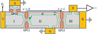
Figure 1: (color on-line) Measurement scheme. S,D and G denote source drain and ground, respectively. The green and the red lines represent the inner and outer edge channels in FF $\nu=2$, respectively. A tunneling of an electron in the inner channel through QPC1 evolves into propagating slow and fast modes with fractional positive and negative charges on both channels, as represented by the small bulges above and below the channels lines

In this Letter a different approach is taken, by considering a mesoscopic device in which the fractional plasma modes impinge on a quantum point contact (QPC) which is placed on their way. The system is sketched in Fig. 1. The 2DEG bulk (the gray area) is assumed to be in a quantum Hall state with FF $\nu=2$, with two copropagating edge channels on each edge of the 2DEG. We assume that no tunneling events occur between the two channels. The source contact marked “S” at the top left is biased by voltage $V_{s}$ relative to other contacts, and so it injects a net electron current $I_{s}=\frac{e^{2}}{h}V_{s}$ to each of the two outgoing edge channels, according to Landauer formula Landauer (1957); Büttiker (1988). Those electrons propagate to the right, and impinge on QPC0, which is tuned to selectively transmit fully only the outer channel to a grounded contact, and completely reflect the biased inner channel toward QPC1. QPC1 is tuned to allow small tunneling probability $T_{1}$ of electrons in the inner channel from region $\rm{I}$ to region $\rm{II}$. An extra electron which tunnels to region $\rm{II}$ in the inner edge channel thus propagates along the top edge toward QPC2, presumably in a form of fractional plasma modes. QPC2, in turn, is tuned to allow small electron tunneling probability $T_{2}$ in the outer channel from region $\rm{II}$ to region $\rm{III}$. A tunneling event through QPC2 creates an extra charge on the outer edge channel in region $\rm{III}$, which propagates to the contact at the top right of Fig. 1 and adds temporarily to the current which is picked up by an amplifier.

In the above setup, the fractionalization of the extra electrons in region $\rm{II}$ leads to low-frequency current noise in region $\rm{III}$. Below, I first present a qualitative argument for the existence of this noise. The noise is then calculated as a function the source bias $V_{s}$ at zero temperature in the weak tunneling limit of the QPCs, using the chiral Luttinger liquid theory. It is found that the noise behavior has a crossover; in the limit of large source bias the noise scales as $V_{s}^{1+2\eta}$ where $0<\eta<0.5$ depends on the coupling between the channels (see definition below). In the low bias limit the noise vanishes as fast as $V_{s}^{3}$.

The appearance of the noise can be explained intuitively as follows. Suppose that an electron tunnels to the inner channel in region $\rm{II}$ through QPC1. Because of the interaction between the two channels, the extra charge breaks up into two density modes, both propagating to the right; a fast, “charge-like” mode, with negative fractional charge excitations on both edge channels, and a slow, “dipole-like” mode, with extra negative charge on the inner channel and extra positive charge (holes) on the outer channel (see Fig. 1). When each mode arrives to be near QPC2, it allows temporarily a certain tunneling event from region $\rm{II}$ to region $\rm{III}$, in the outer edge channel. The charge-like mode induces a tunneling probability of an electron above the Fermi level, while the dipole-like mode induces a tunneling probability of a hole below the Fermi level. The two density modes have different velocities, and so they arrive to QPC2 at different times, which are well resolved if the uncertainty in the energy of the tunneling electron is large enough (i.e. for high enough source bias). In this case the two corresponding tunneling events are separated in time and are statistically uncorrelated. As a result, the net extra current in region $\rm{III}$ is expected to be zero on average, with an equal average number of electrons and holes tunneling through QPC2. However as the tunneling events of electrons and holes are random, the current will fluctuate around the zero average, and these fluctuations will have a low-frequency component, similar to the usual Schottky noise from a tunnel barrier.

For a quantitative prediction for the noise, let us model the system by a low-energy effective theory in the lowest Landau level, using the Hamiltonian

$$H=\sum_{R}H_{R}+H_{QPC1}+H_{QPC2}.$$

The index $R$ goes over the regions, $R\in\{\rm{I,II,III}\}$. $H_{R}$ describes the evolution in the two edge channels within region R, corresponding to electrons with spin up and spin down relative to the magnetic field direction, with Coulomb interaction between the channels. In an appropriate choice of gauge, one has ($\hbar=1$)

$$H_{R} = -i\int_{-\infty}^{\infty}dx\left(v_{\rm{in}}\psi_{\rm{in},R}^{\dagger}\frac{\partial}{\partial x}\psi_{\rm{in},R}+v_{\rm{out}}\psi_{\rm{out},R}^{\dagger}\frac{\partial}{\partial x}\psi_{\rm{out},R}\right)$$ (1)

$$+\frac{u}{2\pi}\int_{-\infty}^{\infty}dx:\rho_{\rm{in},R}\rho_{\rm{out},R}:+\delta_{R,1}eV_{s}\int_{-\infty}^{\infty}dx:\rho_{\rm{in},R}:.$$

Here $\psi_{\rm{in}(out),R}\left(x,t\right)$ is the electron annihilation operator in region $R$ in the inner (outer) channel (the Heisenberg picture is used throughout the Letter) and $\rho_{\rm{in}(out).R}\left(x,t\right)\equiv\psi_{\rm{in}(out),R}^{\dagger}\psi_{\rm{in}(out),R}$ are the 1d electron number densities at the channels. ’:’ denotes normal ordering, $v_{\rm{in}}$ and $v_{\rm{out}}$ are the bare velocities of the two channels and $u$ is the interaction strength. The grounded contacts are modeled effectively by setting the integral boundaries to $\pm\infty$. The last term in Eq. (1) models the bias $eV_{S}$ of the inner channel in region $\rm{I}$ after QPC0.

$H_{QPC1}$ describes the tunneling at QPC1, at $x=0$, between the inner channels in regions $\rm{I}$ and $\rm{II}$. $H_{QPC2}$ describes the tunneling at QPC2, at $x=L,$ between the outer channels of regions $\rm{II}$ and $\rm{III}$. They are given by

$$H_{QPC1}=\bar{v}_{\rm{in}}\sqrt{T_{1}}\psi_{\rm{in},II}^{\dagger}(0)\psi_{\rm{in},I}(0)+\rm{H.c}.$$ (2)

$$H_{QPC2}=\bar{v}_{\rm{out}}\sqrt{T_{2}}\psi_{\rm{out},III}^{\dagger}(L)\psi_{\rm{out},II}(L)+\rm{H.c.}$$ (3)

Here $T_{1}$ and $T_{2}$ are the electron transmission probabilities of QPC1 and QPC2, respectively. $\bar{v}_{\rm{in}}$ and $\bar{v}_{\rm{out}}$ are the renormalized tunneling density of states in the inner and outer channels, which are assumed here for simplicity to be equal for all three regions. They cancel out in the calculation below and do not appear in the final formula for the noise.

The measured noise in region $\rm{III}$ is given by Martin (2005)

$$S_{f\rightarrow 0}=\int_{-\infty}^{\infty}dt\left\langle\Phi_{eV_{s}}\right|\left\{I_{\rm{out},III}(t),I_{\rm{out},III}(0)\right\}\left|\Phi_{eV_{s}}\right\rangle.$$ (4)

The state $\left|\Phi_{eV_{s}}\right\rangle$ is the ground state of the unperturbed Hamiltonian $H_{R}$ (i.e. with no tunneling events between the various regions), where the inner channel of region $\rm{I}$ is biased by $eV_{s}$ and all other edge channels are grounded. The current operators in Eq. (4), $I_{\rm{out},III}\equiv e\frac{d}{dt}\int_{-\infty}^{\infty}dx\rho_{\rm{out},III}$, can be written using the tunneling operators,

$$I_{\rm{out},III}(t)=i\bar{v}_{\rm{out}}\sqrt{T_{2}}\left[\psi_{\rm{out},III}^{\dagger}(L,t)\psi_{\rm{out},II}(L,t)-\rm{H.c.}\right].$$ (5)

The noise is calculated by expanding the time evolution of the current operators to first order in each of the tunneling probabilities $T_{1}$ and $T_{2}$ using Keldysh formalismKeldysh (1964); Rammer and Smith (1986).

The evolution in region $\rm{II}$ is solved analytically. Note that given the Hamiltonian $H_{R=II}$ in Eq. (1), The equation of motion for the density is given by

$$\frac{\partial}{\partial t}\left(\begin{array}[]{c}\rho_{\rm{in},II}\\ \rho_{\rm{out},II}\end{array}\right)+U\frac{\partial}{\partial x}\left(\begin{array}[]{c}\rho_{\rm{in},II}\\ \rho_{\rm{out},II}\end{array}\right)=0,$$ (6)

where U= $\left(\begin{array}[]{cc}v_{\rm{in}}&u\\ u&v_{\rm{out}}\end{array}\right)$ is the velocity matrix. The density modes of the dynamics are the eigenstates of $U$, which can be written in an orthonormal basis as $\left(\begin{array}[]{c}\cos\theta\\ \sin\theta\end{array}\right)$ and $\left(\begin{array}[]{c}\sin\theta\\ -\cos\theta\end{array}\right)$, where $0<\theta<\pi/2$. The velocities of the density modes are the eigenvalues of U,

$$v_{1,2}=\frac{v_{\rm{in}+}v_{\rm{out}}}{2}\pm\sqrt{\frac{1}{4}\left(v_{\rm{in}}-v_{\rm{out}}\right)^{2}+u^{2}},$$ (7)

where the $+(-)$ sign refers to the fast(slow) mode.

The noise in Eq. (4) is now calculated in two steps. First, we expand the time evolution of the current operators to second order in $\sqrt{T_{2}}$. Using Fourier transform to express the result as integral over energies, one finds

$$S_{f\rightarrow 0}=2g_{0}T_{2}\int_{0}^{\infty}d\omega n_{L}(\omega)+2g_{0}T_{2}\int_{-\infty}^{0}d\omega\left(1-n_{L}(\omega)\right),$$ (8)

where $g_{0}=\frac{e^{2}}{h}$ is the unit conductance, and the function $n_{L}(\omega)$ is given by the correlator

$$n_{L}(\omega)=\bar{v}_{\rm{out}}\left\langle\Phi_{eV_{s}}\right|\psi_{\rm{out},II}^{\dagger}(L,0)\psi_{\rm{out},II}(L,t)\left|\Phi_{eV_{s}}\right\rangle_{\rm{FT}},$$ (9)

where “FT” denotes Fourier transform. $n_{L}(\omega)$ can be interpreted as the effective mean occupation of electron states at energy $\omega$ in the outer channel in region $\rm{II}$ at $x=L$, near QPC2. Without inter-channel interaction, in the case $u=0$, $n_{L}(\omega)$ would be a Fermi distribution at zero temperature, which is a step function $n_{L}(\omega)=\Theta\left(-\omega\right)$. However, when $u\neq 0$, the noisy inner channel excites the electrons in the outer channel and changes its occupation distribution function. One can write

$$n_{L}(\omega)=\int_{-\infty}^{\infty}\frac{d\omega_{\rm{out}}}{2\pi}\Theta\left(-\omega+\omega_{\rm{out}}\right)B\left(\omega_{\rm{out}}\right).$$ (10)

The function $B\left(\omega_{\rm{out}}\right)$ is related to the probability for an electron-hole excitation with energy $\omega_{\rm{out}}$ in the outer channel in region $\rm{II}$. In the absence of net current in the outer channel, the electrons and the holes contribute equally to the noise. We can therefore consider only the first term in Eq. (8) twice, which leads to

$$S_{f\rightarrow 0}=4g_{0}T_{2}\int_{0}^{\infty}\frac{d\omega_{\rm{out}}}{2\pi}\omega_{\rm{out}}B(\omega_{\rm{out}}).$$ (11)

The second step is to calculate the function $B(\omega_{\rm{out}})$ up to second order in the transmission amplitude of QPC1, $\sqrt{T_{1}}$, using the chiral Luttinger liquid theory (see supplementary material for details). One finds

$$B(\omega_{\rm{out}})=T_{1}\tau\int_{0}^{e\tilde{V_{s}}}\frac{d\tilde{\omega}_{\rm{in}}}{2\pi}\left(e\tilde{V_{s}}-\tilde{\omega}_{\rm{in}}\right)C\left(\tilde{\omega}_{\rm{out}},\tilde{\omega}_{\rm{in}}\right).$$ (12)

Here $\tau=\frac{L}{v_{2}}-\frac{L}{v_{1}}$ is the relative delay of the arrival of the two modes from QPC1 to QPC2. We define the second mode to be the dipole-like mode, such that $\tau>0$. In Eq. (12) we also have $e\tilde{V_{s}}=eV_{s}\tau$, and $\tilde{\omega}_{\rm{out}}=\omega_{\rm{out}}\tau$.

The function $C\left(\tilde{\omega}_{\rm{out}},\tilde{\omega}_{\rm{in}}\right)$ weights the contribution of processes with energy loss $\tilde{\omega}_{\rm{in}}/\tau$ in the inner channel to the probability of electron-hole excitations with energy $\tilde{\omega}_{\rm{out}}/\tau$ in the outer channel. Note, however, that this function can have negative values. It does not depend on the bias, and is a property of the free evolution of the two modes from $x=0$ to $x=L$. It is found to be a sum of three terms, $C\left(\tilde{\omega}_{\rm{out}},\tilde{\omega}_{\rm{in}}\right)=C^{(2)}+C^{(3)}+C^{(4)}$, with

$$C^{(2)} = \left(2\pi\right)\left|W\left(\tilde{\omega}_{\rm{out}}\right)\right|^{2}\delta\left(\tilde{\omega}_{\rm{in}}-\tilde{\omega}_{\rm{out}}\right)$$ (13)

$$C^{(3)} = 2\Re\left\{e^{i(-\tilde{\omega}_{\rm{in}}+\tilde{\omega}_{\rm{out}})}W\left(\tilde{\omega}_{\rm{in}}\right)W\left(\tilde{\omega}_{\rm{in}}-\tilde{\omega}_{\rm{out}}\right)W^{*}\left(\tilde{\omega}_{\rm{out}}\right)\right\}$$

$$C^{(4)} = e^{i(\tilde{\omega}_{\rm{in}}+\tilde{\omega}_{\rm{out}})}\int\frac{d\omega}{2\pi}e^{-i2\tilde{\omega}}W\left(\tilde{\omega}\right)W^{*}\left(\tilde{\omega}_{\rm{in}}-\tilde{\omega}\right)$$ (14)

$$\times W\left(-\tilde{\omega}_{\rm{out}}+\tilde{\omega}\right)W^{*}\left(\tilde{\omega}_{\rm{in}}-\tilde{\omega}+\tilde{\omega}_{\rm{out}}\right),$$

where $W\left(\tilde{\omega}\right)=w(\tilde{t}){}_{FT}$, and

$$w(\tilde{t})=\frac{(\tilde{t}+1+i\delta)^{\eta}}{(\tilde{t}+i\delta)^{\eta}}-1.$$ (15)

The power $\eta$ is related to the density modes of Eq. (6), $\eta=\cos{\theta}\sin{\theta}=4u/\sqrt{\left(v_{1}-v_{2}\right)^{2}+4u^{2}}$. Thus, the function $W\left(\tilde{\omega}\right)$ is directly related to the fractionalization effect. Fig. (2) shows the function $W\left(\tilde{\omega}\right)$ for three possible values of the power $\eta$. Note that it vanishes at negative values, and satisfies $W(0^{+})=2\pi i\eta$. Also note that the power-law tail of $W\left(\tilde{\omega}\right)$ at high energies is directly related to the power-law divergence of $w(\tilde{t})$ at $t=0$. The asymptotic behavior is $W\left(\tilde{\omega}\gg 1\right)\approx\frac{2\pi\eta}{\Gamma(1+\eta)}\omega^{\eta-1}$, where $\Gamma$ is the gamma function.

Figure 2: (color online) $W(\tilde{\omega})$, absolute value and phase, for $\eta=0.5$ (magenta), $\eta=0.3$ (blue) and $\eta=0.05$ (black)

The fractionalization noise $S_{f\rightarrow 0}$, calculated according to Eqs. (11)-(15), is plotted in Fig. 3 as a function of $e\tilde{V}_{s}$. The contribution of the noise only from $C^{(2)}$ is also plotted in Fig. 3.

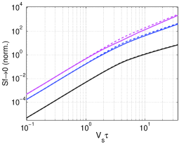
Figure 3: (color on-line) The fractionalization noise, $S_{f\rightarrow 0}/(2g_{0}T_{1}T_{2}\tau^{-1})$ as a function of $\tilde{eV_{s}}=eV_{s}\tau$, for $\eta=0.5,0.3,0.05$ (magenta, blue and black solid lines, respectively). The corresponding dashed lines show the contribution of the term $C^{(2)}$ to the noise for the same values of $\eta$.

In the limit of small bias, $e\tilde{V}_{s}\ll 1$, the leading order of the noise comes from the contribution of $C^{(2)}$ at small values of $\tilde{\omega}_{\rm{in}}$, that is from the value of $|W\left(0^{+}\right)|^{2}$. Equations (11) and (12) then lead to

$$S_{f\rightarrow 0}|_{\tilde{V}_{s}\ll 1}\approx\frac{4\pi\eta^{2}}{3}g_{0}T_{1}T_{2}\tau^{-1}\left(e\tilde{V_{s}}\right)^{3}.$$ (16)

In the opposite limit, of $e\tilde{V}_{s}\gg 1$, The noise is a power-law function of the bias. One can see from Fig. 3 that still the main contribution to the noise comes from $C^{(2)}$. In this limit the noise is dominated by the tail of $\left|W\left(\tilde{\omega}_{\rm{out}}\right)\right|^{2}$ at high $\tilde{\omega}_{\rm{in}}$. Approximating $C\approx C^{(2)}$ and using again Eq. (13) in Eqs. (11) and (12), one finds for this limit

$$S_{f\rightarrow 0}\approx 2g_{0}T_{1}T_{2}\tau^{-1}\frac{2\pi\eta}{\left(2\eta+1\right)\left[\Gamma(1+\eta)\right]^{2}}\left(e\tilde{V}_{s}\right)^{1+2\eta}.$$ (17)

In summary, the low-frequency noise due to the fractionalization effect was calculated in the integer quantum Hall effect at FF $\nu=2$ at zero temperature. The noise is a result of the fractional density modes impinging on a QPC and inducing excess tunneling events of electrons and holes through the QPC to the outgoing leads. The fractionalization noise is found to vanish faster at the low source bias limit, where the time of arrival of the two density modes to QPC2 is no longer well resolved. Thus, the bias in which the crossover occurs in the behavior of the noise corresponds to the difference in the arrival times of the modes from QPC1 to QPC2, $eV_{s}|_{\rm{crossover}}\approx\hbar\tau^{-1}$. This crossover bias may be roughly estimated, based on energy scales which appeared in recent experimental results Altimiras et al. (2010); Neder et al. (2007); Roulleau et al. (2008). If they are indeed related to the same fractionalization effect, then the energy scale is at the order $\approx 10\,\mu eV$ for a device with typical length of $10\,\mu m$. The crossover voltage should be different for devices with different typical lengths and different edge profiles. Finally, it should be mentioned that the effect of finite temperature and the effect of the disorder in the edge channels in region II on the behavior of the noise were not discussed in the model above and deserves future study.

I acknowledge B. I. Halperin, G. Viola, Y. Oreg and E. Berg for very useful discussions. This work was supported by NSF grant DMR-0906475.

References

- Su et al. (1979) W. P. Su, J. R. Schrieffer, and A. J. Heeger, Phys. Rev. Lett. 42, 1698 (1979).
- Laughlin (1983) R. B. Laughlin, Phys. Rev. Lett. 50, 1395 (1983).
- Pham et al. (2000) K.-V. Pham, M. Gabay, and P. Lederer, Phys. Rev. B 61, 16397 (2000).
- Steinberg et al. (2008) H. Steinberg, G. Barak, A. Yacoby, L. N. Pfeiffer, K. W. West, B. I. Halperin, and K. Le Hur, Nature-Physics 4, 116 (2008).
- Kane and Fisher (1994) C. L. Kane and M. P. A. Fisher, Phys. Rev. Lett. 72, 724 (1994).
- Saminadayar et al. (1997) L. Saminadayar, D. C. Glattli, Y. Jin, and B. Etienne, Phys. Rev. Lett. 79, 2526 (1997).
- de Picciotto et al. (1997) R. de Picciotto, M. Reznikov, M. Heiblum, V. Umansky, G. Bunin, and D. Mahalu, Nature 389, 162 (1997).
- Halperin (1982) B. I. Halperin, Phys. Rev. B 25, 2185 (1982).
- Altimiras et al. (2010) C. Altimiras, H. le Sueur, U. Gennser, A. Cavanna, D. Mailly, and F. Pierre, Phys. Rev. Lett. 105, 226804 (2010).
- Rohrlich et al. (2007) D. Rohrlich, O. Zarchin, M. Heiblum, D. Mahalu, and V. Umansky, Phys. Rev. Lett. 98, 096803 (2007).
- Neder et al. (2007) I. Neder, F. Marquardt, M. Heiblum, D. Mahalu, and V. Umansky, Nature-Physics 3, 534 (2007).
- Roulleau et al. (2008) P. Roulleau, F. Portier, P. Roche, A. Cavanna, G. Faini, U. Gennser, and D. Mailly, Phys. Rev. Lett. 101, 186803 (2008).
- Levkivskyi and Sukhorukov (2008) I. P. Levkivskyi and E. V. Sukhorukov, Phys. Rev. B 78, 045322 (2008).
- Neder et al. (2006) I. Neder, M. Heiblum, Y. Levinson, D. Mahalu, and V. Umansky, Phys. Rev. Lett. 96, 016804 (2006).
- Berg et al. (2009) E. Berg, Y. Oreg, E.-A. Kim, and F. von Oppen, Phys. Rev. Lett. 102, 236402 (2009).
- Horsdal et al. (2011) M. Horsdal, M. Rypestøl, H. Hansson, and J. M. Leinaas, Phys. Rev. B 84, 115313 (2011).
- Mahé et al. (2010) A. Mahé, F. D. Parmentier, E. Bocquillon, J.-M. Berroir, D. C. Glattli, T. Kontos, B. Placais, G. Fève, A. Cavanna, and Y. Jin, Phys. Rev. B 82, 201309 (2010).
- Landauer (1957) R. Landauer, IBM J. Res. Dev. 1, 223 (1957).
- Büttiker (1988) M. Büttiker, Phys. Rev. B 38, 9375 (1988).
- Martin (2005) T. Martin (Elsevier, 2005), vol. 81 of Les Houches Summer School Proceedings, pp. 283 – 359.
- Keldysh (1964) L. V. Keldysh, Zh. Eksp. Teor. Fiz. 47, 1515 (1964).
- Rammer and Smith (1986) J. Rammer and H. Smith, Rev. Mod. Phys. 58, 323 (1986).