The Spitzer Spectroscopic Survey of the Small Magellanic Cloud (S⁴MC): Probing the Physical State of Polycyclic Aromatic Hydrocarbons in a Low-Metallicity Environment

Abstract

We present results of mid-infrared spectroscopic mapping observations of six star-forming regions in the Small Magellanic Cloud from the Spitzer Spectroscopic Survey of the SMC (S⁴MC). We detect the mid-IR emission from polycyclic aromatic hydrocarbons (PAHs) in all of the mapped regions, greatly increasing the range of environments where PAHs have been spectroscopically detected in the SMC. We investigate the variations of the mid-IR bands in each region and compare our results to studies of the PAH bands in the SINGS sample and in a sample of low-metallicity starburst galaxies. PAH emission in the SMC is characterized by low ratios of the 6$-$9 µm features relative to the 11.3 µm feature and weak 8.6 and 17.0 µm features. Interpreting these band ratios in the light of laboratory and theoretical studies, we find that PAHs in the SMC tend to be smaller and less ionized than those in higher metallicity galaxies. Based on studies of PAH destruction, we argue that a size distribution shifted towards smaller PAHs cannot be the result of processing in the interstellar medium, but instead reflects differences in the formation of PAHs at low metallicity. Finally, we discuss the implications of our observations for our understanding of the PAH life-cycle in low-metallicity galaxies—namely that the observed deficit of PAHs may be a consequence of PAHs forming with smaller average sizes and therefore being more susceptible to destruction under typical interstellar medium conditions.

1. Introduction

The mid-infrared emission from normal star-forming galaxies is characterized by a series of bright emission bands at approximately 3.3, 6.2, 7.7, 8.6 and 11.3 µm, with weaker features at surrounding wavelengths. Laboratory work has shown a close correspondence between the interstellar emission features and the vibrational modes of the carbon-carbon (C-C) and carbon-hydrogen (C-H) bonds in polycyclic aromatic hydrocarbons (PAHs; Léger & Puget 1984; Allamandola et al. 1985, 1989). Although there is not a definitive laboratory identification of the mid-IR band carrier or population of carriers, it is considered very likely that these features arise from the vibrational de-excitation of PAHs with a range of sizes after absorbing UV or optical photons (for a recent review, see Tielens 2008).

The widespread observation of the emission bands in the Milky Way and elsewhere suggests that PAHs are an abundant and energetically important component of interstellar dust (emitting $\sim 10$% of the total infrared emission from a galaxy; Helou et al. 2000; Smith et al. 2007b). In addition, PAHs play a number of important roles in the interstellar medium (ISM). They are a major source of photoelectric heating (Bakes & Tielens 1994; Wolfire et al. 1995; Hollenbach & Tielens 1999; Helou et al. 2001) and participate in chemical reaction networks (Bakes & Tielens 1998; Wolfire et al. 2008; Wakelam & Herbst 2008) in a variety of ISM phases. Because of these crucial roles, we would like to understand how and why the characteristics of PAHs depend on galaxy properties such as metallicity and star-formation history and what specific factors control the abundance, size distribution and physical state (ionization, hydrogenation, compactness, symmetry, etc.) of PAHs in the ISM.

The physical state of a population of PAHs is reflected in the relative intensities, profile shape and central wavelength of the mid-IR emission bands. Of the major PAH bands, laboratory spectroscopy has suggested that those at 3.3, 8.6 and 11$-$14 µm arise from C-H stretching and bending modes while the 6.2 and 7.7 complexes are from C-C stretching. Longer wavelength features like the 17.0 µm complex are most likely related to more complex ring bending modes of the molecule (Moutou et al. 2000). The relative strengths of these bands for a given population of PAHs will depend on their size distribution and physical state allowing us diagnostics of the PAH population from mid-IR spectroscopy.

For instance, laboratory and theoretical investigations have consistently shown that the C-H out-of-plane bending modes between 11$-$15 µm in ionized PAHs are weak, while they are strong in neutral PAHs. The opposite is true of the C-C stretch and C-H in-plane bending modes between $6-9$ µm (Szczepanski & Vala 1993; Hudgins et al. 1994), so the ratios of these two sets of features should trace PAH ionization to some degree. Recent work by Galliano et al. (2008a) argued that the variations of the 6.2, 7.7, 8.6 and 11.3 µm features within and between galaxies are consistent with being controlled by ionization. Specifically, they find that the ratios of 6.2, 7.7 and 8.6 to the 11.3 µm bands are correlated over an order-of-magnitude, while ratios such as 7.7/6.2 and 8.6/6.2 stay roughly constant as a function of the 7.7/11.3 ratio.

The ratios of short-to-long wavelength PAH bands, however, are also expected to depend on the PAH size distribution (Draine & Li 2001), such that small PAHs emit more strongly in shorter wavelength features. In addition to this general trend, laboratory and theoretical studies have suggested that some specific features originate from large PAHs. Peeters et al. (2004) find that large PAHs are required to reproduce the general characteristics of the 17.0 µm complex, although the charge state of the carrier is not well determined. Recent work by Bauschlicher et al. (2008, 2009) has suggested that the strength of the 8.6 µm band also is an indicator of the contribution of large PAHs to the mid-IR spectrum. They find that in their theoretical investigations of the spectrum of large compact and irregular PAHs, only large, charged, compact PAHs have a feature at 8.6 µm that can reproduce the interstellar band.

Finally, as reviewed in detail by Hony et al. (2001) and Bauschlicher et al. (2009), the relative strengths of the 11$-$15 µm C-H out-of-plane bending modes provide information about the structure of PAHs. The type of structure adjacent to the vibrating C-H bond determines the wavelength of the mode. If a given aromatic carbon ring on the edge of a PAH has only one attached hydrogen (out of four possible for a PAH that consists of more than one aromatic ring), while the rest of the bonds are connected to other aromatic rings, it is considered a “solo” hydrogen. If two of the possible sites contain C-H bonds, this is considered a “duo”, and the “trio” and “quartet” are similarly defined. In structural terms, straight edges produce “solo” hydrogens while corners produce “duo” hydrogens. Irregularities like bays and linear extensions produced “trio” and “quartet” hydrogens. These different modes have different wavelengths (dependent on the size of the molecule; Bauschlicher et al. 2009). Thus, observations of the strengths of the 11$-$15 µm features can provide information about the PAH structure.

Using the knowledge of PAH bands gained from these laboratory and theoretical studies, it is possible to diagnose the physical state of PAHs in extragalactic environments observed with ISO and Spitzer. In particular, evidence for changes in PAH properties with radiation field intensity and metallicity have been seen in a variety of studies:

• Galliano et al. (2008a) studied the variation of the ratios of the 6.2, 7.7, 8.6 and 11.3 bands in a diverse sample of galaxies and individual star-forming regions and found variations in the 6$-$9 vs 11.3 µm features correlated with the local UV field strength—a trend they interpreted as arising mainly from changes in the PAH ionization state.

• Smith et al. (2007b) have found that PAH emission from AGN-hosting galaxy nuclei shows very low 7.7/11.3 ratios (see also O’Dowd et al. 2009; Diamond-Stanic & Rieke 2010; Wu et al. 2010). Some studies have also found that the spectra of these sources also show average or even high ratios of the 17.0 feature to the 7.7 and 11.3 bands (Smith et al. 2007b; O’Dowd et al. 2009). These trends have been interpreted as the preferential destruction of small PAHs by the hard radiation field produced by the AGN, leading to decreased emission in the short wavelength bands relative to the long wavelength bands.

• Hunt et al. (2010) studied the PAH features in a sample of blue compact dwarfs (BCDs) with a range of metallicities and found evidence for increased strengths of the 8.6 and 11.3 features relative to the other PAH bands in these intensely star-forming galaxies. They interpreted these trends as evidence for destruction of small PAHs in the harder, more intense radiation fields of these galaxies citing recent theoretical work by Bauschlicher et al. (2008) which suggests that the 8.6 µm feature arises predominantly from large PAHs.

• Smith et al. (2007b) measured the integrated PAH band strengths in the central regions of galaxies in the SINGS sample and found indications that the 17.0 µm complex is weak compared to the other PAH bands at low-metallicity, although their sample contains few low-metallicity galaxies.

• Resolved studies of PAH emission in the Magellanic Clouds have also shown variations in the band ratios. For instance, Reach et al. (2000) detected PAH emission from the quiescent molecular clouds SMC B1 #1 with a very low 7.7/11.3 ratio. Li & Draine (2002) found that they could not reproduce the SMC B1 ratio using their Milky Way PAH model.

In addition to these changes in the PAH physical state, observations with ISO and Spitzer have demonstrated that the fraction of PAHs relative to the total amount of dust decreases in low-metallicity environments (Madden 2000; Engelbracht et al. 2005; Madden et al. 2006; Wu et al. 2006; Draine et al. 2007; Gordon et al. 2008; Hunt et al. 2010; Lebouteiller et al. 2011). A number of explanations for the PAH deficit in low-metallicity galaxies have been proposed including a time lag between the formation of PAHs in AGB star atmospheres relative to SNe-produced dust (Galliano et al. 2008b), destruction of PAHs by supernova shocks (O’Halloran et al. 2006) and destruction of PAHs by harder and/or more intense UV fields (Madden et al. 2006; Gordon et al. 2008). Recent work by Sandstrom et al. (2010) (Paper I) on the fraction of PAHs in the Small Magellanic Cloud has shown a very low PAH fraction in the diffuse ISM of this low-metallicity galaxy and a PAH fraction in dense gas within a factor $\sim 2$ of the Milky Way. They argue that PAHs are destroyed in the diffuse ISM of the SMC and may be forming in dense regions. Thus, in addition to variations in the destruction of PAHs, it is possible that as a function of metallicity the balance between AGB-produced PAHs and PAHs that form in the ISM may change.

These proposed variations in the life-cycle of PAHs in low-metallicity galaxies will be reflected in changes to the physical state of the PAHs themselves — their size distribution, hydrogenation, ionization state, chemical substitutions and/or functional groups and structural characteristics. Enhanced destruction of PAHs by UV fields or shocks should change the PAH size distribution, since smaller molecules are easier to photodissociate (Allain et al. 1996a, b; Le Page et al. 2001). If the dominant formation mechanism of PAHs changes as a function of metallicity it may be reflected in the size distribution and irregularity of the molecules. Thus, by observing the physical state of PAHs in a low-metallicity environment we hope to understand what drives the observed differences in the PAH life-cycle.

To that end, we present the results of a mid-IR spectroscopic survey of PAH emission in the Small Magellanic Cloud (SMC). At a distance of 61 kpc (Hilditch et al. 2005) and with a metallicity of $12+$ log(O/H) $\sim 8.0$ (Kurt & Dufour 1998), the SMC presents the ideal target to understand the properties of PAHs in low-metallicity systems at high spatial resolution. The SMC represents an intermediate case between Galactic sources where variations can be studied within objects (Hony et al. 2001; Peeters et al. 2002; Rapacioli et al. 2005; Berné et al. 2007) and other galaxies where only galaxy-wide results are obtained. The Spitzer Spectroscopic Survey of the SMC (S⁴MC) consists of low-resolution spectral mapping observations using the Infrared Spectrograph (IRS) on Spitzer over six of the major star-forming regions of the SMC. In Paper I, we presented the results of SED and spectral fitting using the S⁴MC data to determine the PAH fraction across the galaxy. In this paper we turn our attention to using the band ratios to learn about the physical state of PAHs.

In Section 2 we describe the S⁴MC observations and data reduction. Section 2.5 covers the spectral fitting. In Section 3 we describe the variations in the band ratios in the six star-forming regions in our sample and finally in Section 4 we discuss what the variations tell us about the physical state of SMC PAHs and in Section 5.1, the implications of our results for understanding the PAH deficiency in low-metallicity galaxies.

2. Spitzer Spectroscopic Survey of the Small Magellanic Cloud (S⁴MC)

We mapped six star-forming regions in the SMC using the low-resolution orders of the InfraRed Spectrograph (IRS) on Spitzer as part of the S⁴MC project (GO 30491—now combined with a larger mosaic of the galaxy as part of SAGE-SMC; Bolatto et al. 2007, Gordon et al. 2011, submitted). Figure 1 shows the coverage of our spectral maps overlaid on the S³MC 24 µm mosaic (Bolatto et al. 2007). Figures 2, 3 and 4 show three-color images of the six regions, overlaid with the coverage of all of the orders. These regions are all displayed with the same color scale. In the following analysis, we are limited to the regions with coverage in both of the SL orders because of our focus on the PAH emission bands. We list the details of the observations in Table 1.

The regions we have mapped were selected to cover a range of properties and therefore represent a diverse sample of SMC sources. The N 66 field covers the well studied giant H II region NGC 346, which hosts 33 O stars (Massey et al. 1989). ISO observations of N 66 by Contursi et al. (2000) show radiation field intensity upwards of $10^{5}$ times the solar neighborhood radiation field in some of the brightest mid-IR peaks. We have also mapped the quiescent molecular region SMC B1 #1, found in the SW Bar (Rubio et al. 1993). This was the first location where PAH emission was detected spectroscopically in the SMC by Reach et al. (2000). Also in the SW Bar region, we map three other fields: N22, a compact H II region surrounded by molecular gas; SW Bar 1, a region of active, but more evolved, star-formation (including the N 27 nebula), with bright 8 µm and H$\alpha$ emission; and SW Bar 3, which covers regions of molecular gas and recent star-formation. In the Wing of the SMC, we map the N 83/N 84 complex, which covers a region of high UV field intensity with abundant molecular gas (Leroy et al. 2009). Finally, in the N 76 region our map covers a young supernova remnant 1E 0102.2$-$7219 (Stanimirović et al. 2005; Sandstrom et al. 2009), a Wolf-Rayet nebula and a few small regions of molecular gas on the outskirts of the nebula.

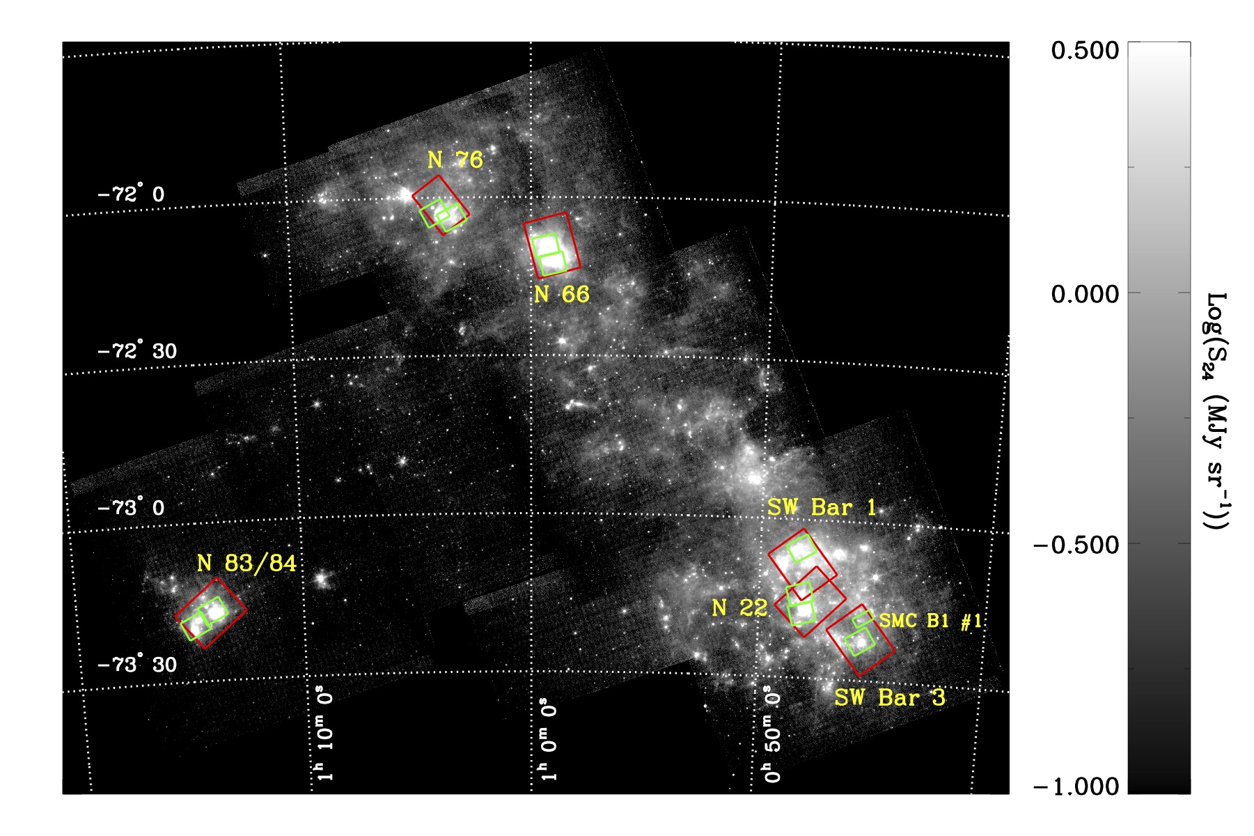
Figure 1.— The coverage of the S⁴MC survey overlayed on the MIPS 24 µm map from S³MC. The color scale is logarithmic, with the stretch illustrated in the colorbar. The red boxes show the coverage of the LL1 order maps (the LL2 maps are shifted by $\sim 3\arcmin$) and the green boxes show the coverage of the SL1 order maps (the SL2 maps are shifted by $\sim 1\arcmin$). We also identify the various regions of the galaxy by the names we will refer to in the remainder of this paper.

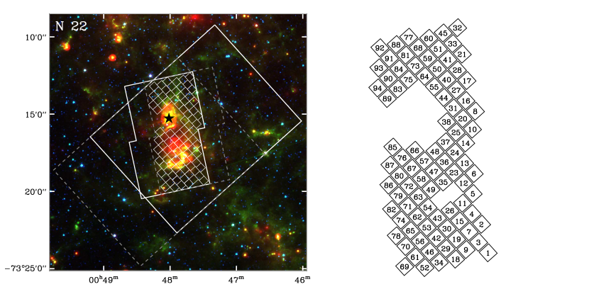
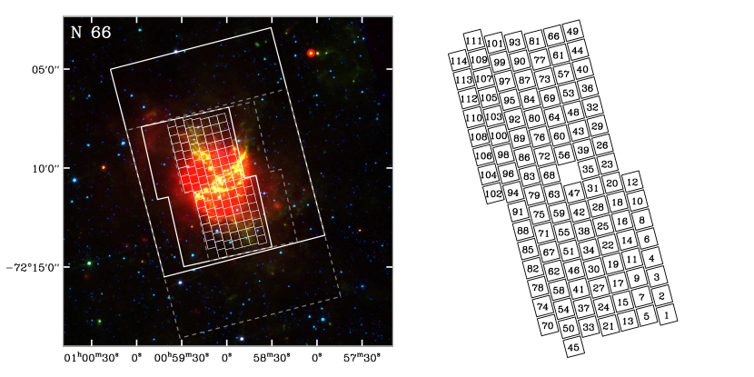
Figure 2.— Coverage of the S⁴MC observations in the N 22 and N 66 regions. The three-color images are constructed from S³MC photometry in the IRAC 3.6 (blue), IRAC 8.0 (green) and MIPS 24 (red) bands. The color table is the same in Figures 2,  3 and  4. The coverage of the LL1 and SL1 orders is shown with a solid white line while the LL2 and SL2 coverage is shown with a gray dashed line. For the following analysis we are limited to regions with coverage in both SL bands. The white boxes illustrate locations where we have extracted spectra from the cube for this analysis (see the text for details) and the right panel shows all of the extracted regions along with a number identifying them. There is a very bright point source in the N 22 region which is saturated in the 24 µm MIPS observation, we show its location with a black star. Because of the artifacts associated with bright point sources we are forced to omit some regions from our analysis.

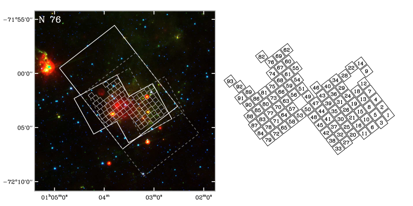
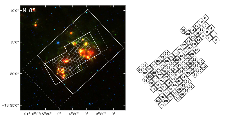
Figure 3.— Coverage of the S⁴MC observations in N 76 and N 83. The images and color table are the same as in Figure 2. In N 76, we avoid the region dominated by the supernova remnant 1E 0102.2$-$7219 (visible as a ring-like feature in the 24µm band; Sandstrom et al. 2009, presented an analysis of the IRS observations for this region). In N 83, most of the area of the northern SL cubes are affected by artifacts due to the saturation of the peak-up array due to a very bright point source in the region. We avoid those areas in selecting the extraction regions.

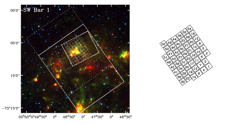
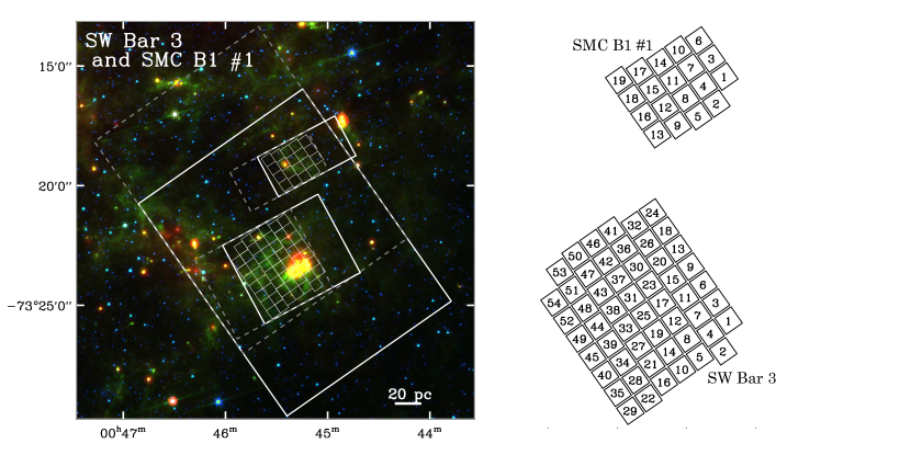
Figure 4.— Coverage of the S⁴MC observations in the SW Bar 1 and 3 regions. The images and color table are the same as in Figure 2. The coverage of the SMC B1 spectral map is shown in the SW Bar 3 region.

Table 1S⁴MC Observations

Region	R. A. (J2000)	Dec. (J2000)	Observation Date	AOR Number
LL Observations
SW Bar 3	$0^{\rm h}45^{\rm m}23^{\rm s}$	$-73^{\circ}22\arcmin 00\arcsec$	11 Jun 2007	18264832
N 22	$0^{\rm h}47^{\rm m}42^{\rm s}$	$-73^{\circ}15\arcmin 06\arcsec$	09 Sep 2006	18261504
SW Bar 1	$0^{\rm h}48^{\rm m}08^{\rm s}$	$-73^{\circ}08\arcmin 24\arcsec$	11 Jun 2007	18264576
N 66	$0^{\rm h}59^{\rm m}09^{\rm s}$	$-72^{\circ}09\arcmin 14\arcsec$	15 Nov 2006	18262272
N 76	$1^{\rm h}03^{\rm m}41^{\rm s}$	$-72^{\circ}01\arcmin 30\arcsec$	12 Dec 2006	18263040
N 83/84	$1^{\rm h}14^{\rm m}05^{\rm s}$	$-73^{\circ}17\arcmin 00\arcsec$	10 Sep 2006	18263808
SL Observations
SW Bar 3	$0^{\rm h}45^{\rm m}26^{\rm s}$	$-73^{\circ}22\arcmin 30\arcsec$	10 Jun 2007	18265344
SMC B1 #1	$0^{\rm h}45^{\rm m}21^{\rm s}$	$-73^{\circ}20\arcmin 10\arcsec$	10 Jun 2007	18261248
SW Bar 1	$0^{\rm h}48^{\rm m}13^{\rm s}$	$-73^{\circ}05\arcmin 20\arcsec$	10 Jun 2007	18265088
N 22 North	$0^{\rm h}48^{\rm m}11^{\rm s}$	$-73^{\circ}13\arcmin 56\arcsec$	20 Nov 2006	18262016
N 22 South	$0^{\rm h}48^{\rm m}04^{\rm s}$	$-73^{\circ}17\arcmin 50\arcsec$	20 Nov 2006	18261760
N 66 North	$0^{\rm h}59^{\rm m}22^{\rm s}$	$-72^{\circ}09\arcmin 07\arcsec$	21 Nov 2006	18262784
N 66 South	$0^{\rm h}59^{\rm m}05^{\rm s}$	$-72^{\circ}12\arcmin 50\arcsec$	20 Nov 2006	18262528
N 76 1	$1^{\rm h}03^{\rm m}11^{\rm s}$	$-72^{\circ}04\arcmin 01\arcsec$	09 Dec 2006	18263296
N 76 2	$1^{\rm h}04^{\rm m}00^{\rm s}$	$-72^{\circ}02\arcmin 50\arcsec$	09 Dec 2006	18263552
N 83	$1^{\rm h}14^{\rm m}00^{\rm s}$	$-73^{\circ}16\arcmin 40\arcsec$	10 Dec 2006	18264064
N 84	$1^{\rm h}14^{\rm m}50^{\rm s}$	$-73^{\circ}19\arcmin 20\arcsec$	10 Dec 2006	18264320

2.1. Mapping Strategy and Spectral Cube Construction

The maps were constructed by stepping the IRS slit in a grid of positions parallel and perpendicular to the slit. The maps are fully sampled by stepping by half of a slit width (steps of 1.85″ and 5.08″ for SL and LL, respectively) perpendicular to the slit. The LL maps are composed of a grid of 98 perpendicular and 7 parallel steps, with half slit length steps parallel to the slit and 14 seconds of integration time per position (except N 76 which has 75 $\times$ 6 steps perpendicular and parallel). The LL spectral maps cover an area of $493\arcsec\times 474\arcsec$ ($376\arcsec\times 395\arcsec$ for N 76). The SL maps are constructed similarly except that we use full slit width steps parallel to the slit to increase the mapped area at the expense of some pixel redundancy. All of the SL maps, aside from the map of SMC B1, have 120 perpendicular by 5 parallel pointings ($220\arcsec\times 208\arcsec$) with integration times of 14 seconds per position. We have made a deeper map of SMC B1, the location where PAH emission was first detected from the SMC (Reach et al. 2000) using 60 by 4 slit positions ($109\arcsec\times 156\arcsec$) with 60 second integration times. The spectral coverage of the low-resolution orders extends between 5.2 and 38.5 µm with spectral resolving power ranging between $\sim 60-120$.

Each mapping observation was preceded or followed closely in time by an observation of an “off” position at RA 1^h9^m40^s Dec $-$73^∘31$\arcmin$30$\arcsec$ (J2000). This position was chosen to be free from SMC emission at the level of our MIPS and IRAC mosaics from S³MC. The “off” position was observed with the same ramp times as its corresponding mapping observations using “staring mode”. There were four nod positions in each “off” observation, with 9 repetitions per nod. In the course of processing the maps, the outlier-clipped mean of the 36 two-dimensional spectral images of the “off” position was subtracted from each of the mapping BCDs. This removes the zeroth-order foreground emission from the zodiacal light and Milky Way cirrus as well as mitigating the effects of time-variable rogue pixels in the low-resolution arrays.

We have used the BCDs from pipeline version S15.3 and S16.1 to create our final cubes. There are no significant differences between these two pipeline versions for our purposes. The cubes were assembled using the Cubism software package (v1.7) distributed by the SSC (Smith et al. 2007a). Cubism takes the pipeline processed BCDs as input and uses polygon-clipping based re-projection to transform the two dimensional spectral images into a three dimensional spectral cube. Cubism also propagates the uncertainties associated with the data collection events, known as ramps. We propagate these uncertainties throughout the following analysis, but note that they represent only the statistical uncertainties of each pixel and do not take into account the more important systematic errors. In assembling the cubes in Cubism we apply a “slit-loss correction function” which is essentially an extended source calibration factor for the IRS (Smith et al. 2007a).

We remove bad pixels in the cubes using the tools provided in Cubism. These bad pixels are identified by the stripes they produce in the spectral maps, resulting from the movement of the bad pixel through the grid of positions. The number of bad pixels increases towards the longest wavelengths in the cube, effectively making the spectrum past $\sim 35$ µm have much lower signal-to-noise. Regarding bad pixel flagging, we note that in cases where the core of the PSF of a point source falls on a bad pixel in the detector, there can be difficulties in reconstructing the emission profile in Cubism. This issue is exacerbated by two problems: the spatial under-sampling of the IRS, and the “full-width” steps used to construct the map, which reduces the pixel redundancy. Because we are interested in the diffuse emission, we have performed extensive bad pixel subtraction in order to get the cleanest map of the region without regard to the effects on point sources. For that reason, in the vicinity of bright point sources there can be artifacts that interfere with the determination of the PAH emission band strengths in the spectra of point sources . In the following, we avoid these regions in the cubes, particularly in the core of N 66 and in the vicinity of the bright point sources in N 22 and N 83. In N 83, the brightest point source presents another difficulty in that it saturates the peak-up array, leading to uncorrected droop effects over a large fraction of the map. In our analysis, we have avoided regions affected by this artifact as well.

2.2. Foreground Subtraction

The “off” position observations that were performed close in time to each mapping BCD allow us to subtract the majority of the zodiacal and Milky Way foregrounds from our maps. There are, however, gradients in both foregrounds between the “off” location and the map location. To remove these additional gradients we use the zodiacal light spectrum predicted by the Spitzer Observation Planning Tool (SPOT) at the times of each observation to calculate the difference in the zodiacal foreground between the “off” location and the map location versus wavelength. SPOT uses the zodiacal light model of Kelsall et al. (1998) from DIRBE observations. The modifications to this model for predicting the zodiacal light at Spitzer wavelengths are described in the documentation from the Spitzer Science Center(SSC). To determine the gradient in the Milky Way foreground we assume a correlation between the cirrus dust emission and the column density of neutral hydrogen (as in Boulanger et al. 1996). We use the Draine & Li (2007) emissivity of Milky Way dust and a map of H I from a combined ATCA/Parkes survey (E. Muller, private communication) to measure the Milky Way foreground gradient as in Paper I.

2.3. “Dark Settle” Related Artifacts in the S⁴MC Spectral Mapping

In performing the analysis of the S⁴MC data we discovered that both the SL and LL observations are affected by an artifact related to a time- and position variable residual background level on the detector. This artifact is a general issue in IRS spectral mapping, but is particularly important for faint regions like those we study here. This issue is very similar to what has been seen in LH observations and referred to as the “dark settle” issue. The artifact causes a tilt to the various orders, leading to a mis-match between the spectral orders LL1-LL2 and SL1-SL2 as well as introducing spurious curvature to the spectrum. Because of the faintness of the PAH emission in many SMC regions, this artifact can have a significant effect on the flux in the 7.7 µm complex, located at the overlap of the SL1 and SL2 orders.

Our basic approach to dealing with the artifact is to correct the data at the BCD level by determining the shape of the residual background from the inter-order region. The details of this procedure are described in the Appendix. For the SL orders in particular, the inter-order space is very small, especially since the gap between the SL3 and SL2 orders is strongly affected by the scattered light from the peak-up arrays and its correction in the IRS pipeline. At a basic level, we do not have information about the background level within the spectral orders, which is precisely where we would like to remove it. Therefore, our correction of this artifact is approximate at best and we proceed in the remainder of the paper to deal with two versions of the spectral cubes: one with no correction of the “dark settle” issue and one with a correction we determine from the inter-order light. As described in the Appendix, the technique we use may overcorrect (i.e. by removing too much flux from the 7.7 µm feature). We argue that the uncorrected and corrected spectra should bracket the range of possible values for the band strengths.

2.4. Spectral Extraction and Stitching

In order to get better signal-to-noise for determining the band ratios we extract the spectra in $25\arcsec\times 25$″ boxes. This extraction aperture is also large enough to avoid problems with the variation of the PSF with wavelength (the FWHM of the PSF at 35 µm is $\sim 9$″). We have tiled the cubes in the region of full overlap between all orders with these extraction boxes. The right panels of Figures 2, 3 and 4 show the extraction boxes for each region, excluding those affected by point source artifacts. We refer to the individual spectra by the number shown on these diagrams throughout the paper.

After the correction for foreground gradients and “dark settle”-type artifacts, our extracted spectra show offsets in the overlap of the SL1 and LL2 orders that vary from region to region, but stay relatively constant within a given region. These offsets are additive and on the order of a few tenths of MJy sr^-1. In correcting these offsets we first extract photometry in matching apertures from the S³MC 24 µm mosaic (which has been foreground subtracted as described in Sandstrom et al. 2010) and find the average offset at 24 µm for the MIPS and synthetic IRS photometry for each region. We then use this additive region-based offset to tie the IRS spectrum to the MIPS photometry—a step which is necessary because we have no prior information on which order is “correct” and the 8 µm photometry relies on an extended source correction for IRAC and is thus less reliable than the 24 µm photometry. Next we determine the offset between the SL and LL orders in their overlap region ($\sim 14.3-14.7$ µm) and find another additive region-based correction that we then add to the SL spectra.

After tying the spectra to the MIPS 24 µm photometry and correcting the LL/SL offset, we stitch the spectra together by interpolating the long wavelength end of each order onto the grid of the overlapping shorter wavelength order and averaging the resulting values together. The procedures we employ in correcting offsets between the orders and stitching the spectra together do not significantly affect our results.

2.5. Fitting the PAH Emission Bands

We use the PAHFIT spectral fitting routine (Smith et al. 2007b) to measure the strengths of the PAH emission bands and a variety of emission lines from our spectra. Figure 5 shows the results of fits to some high signal-to-noise spectra from our dataset. PAHFIT uses combinations of Drude profiles to fit the emission bands and Gaussians to fit the emission lines. We do not include extinction in our fits—Lee et al. (2009) found very low levels of mid-IR extinction in the SMC as expected given the galaxy’s low dust-to-gas ratio. The effect of extinction on the band ratios would tend to primarily suppress emission in the 8.6 and 11.3 µm bands because of the silicate extinction feature at 9.7 µm. In the cases where the PAH emission features form a complex (for instance, the 7.7 µm feature), we report only the total and not the properties of the individual components. We have used the default line list provided in PAHFIT with the exception of adding in the Pfund-$\alpha$ recombination line of hydrogen at 7.46 µm, which we see in the spectra of N 66 and some of the spectra in N 22. We perform the fits on the original spectra and on the “dark settle” artifact corrected spectra.

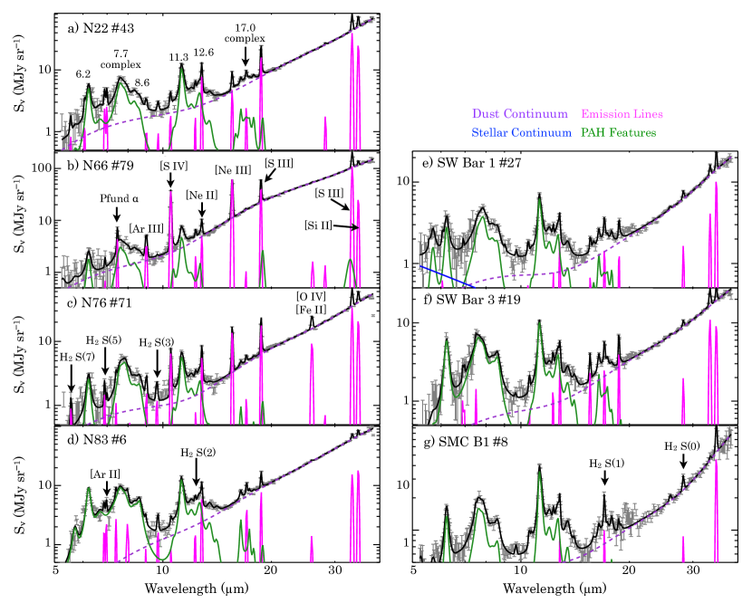
Figure 5.— These plots show example PAHFIT results for spectra from our sample. The spectra are labeled with the region and a number which corresponds to labels on Figures 2,  3 and 4. Each plot shows the spectrum and statistical uncertainties in gray, the full best fit model in black, the PAH contribution to the best fit model in green, the line emission in magenta, the stellar continuum in blue and the dust continuum in orange.

Table 2 lists the measured integrated intensities for the major PAH features as well as the lines of [Ne III] at 15.6 µm and [Ne II] at 12.8 µm for each spectrum extracted from the cubes both with and without the “dark settle” correction.

Table 2Spectral Fit Results

Region	Num	R.A.	Dec.	6.2	7.7	8.3	[Ne II]	[Ne III]
N 22	1	11.891834	$-$73.313254	4.237$\pm$0.527	5.691$\pm$0.778	0.361$\pm$0.371	0.213$\pm$0.052	0.034$\pm$0.019
N 22	2	11.905884	$-$73.299297	1.950$\pm$0.399	4.367$\pm$1.034	0.000$\pm$0.269	0.040$\pm$0.048	0.003$\pm$0.022
N 22	3	11.909261	$-$73.308280	2.895$\pm$0.455	3.297$\pm$0.939	0.000$\pm$0.379	0.031$\pm$0.075	0.031$\pm$0.028
N 22	4	11.923294	$-$73.294323	1.998$\pm$0.295	7.586$\pm$1.009	0.000$\pm$0.331	0.222$\pm$0.057	0.046$\pm$0.020
N 22	5	11.923392	$-$73.284345	6.922$\pm$0.409	14.024$\pm$1.014	1.669$\pm$0.206	0.352$\pm$0.057	0.054$\pm$0.023
N 22	6	11.923489	$-$73.274367	5.214$\pm$0.474	11.883$\pm$0.991	1.311$\pm$0.409	0.301$\pm$0.054	0.069$\pm$0.021
N 22	7	11.926679	$-$73.303306	2.149$\pm$0.448	5.763$\pm$1.168	0.000$\pm$0.346	0.111$\pm$0.065	0.025$\pm$0.018
N 22	8	11.927250	$-$73.243438	5.895$\pm$0.370	10.887$\pm$1.138	0.000$\pm$0.619	0.147$\pm$0.038	0.005$\pm$0.020
N 22	9	11.930068	$-$73.312289	4.740$\pm$0.560	5.598$\pm$0.748	0.255$\pm$0.267	0.081$\pm$0.047	0.035$\pm$0.021
N 22	10	11.930627	$-$73.252421	3.770$\pm$0.355	8.918$\pm$0.942	0.000$\pm$0.564	0.095$\pm$0.051	0.023$\pm$0.016
N 22	11	11.940693	$-$73.289347	4.091$\pm$0.545	12.358$\pm$1.020	0.650$\pm$0.237	0.956$\pm$0.078	0.463$\pm$0.028
N 22	12	11.940781	$-$73.279369	4.818$\pm$0.457	13.174$\pm$0.957	0.978$\pm$0.311	0.410$\pm$0.083	0.081$\pm$0.019
N 22	13	11.940868	$-$73.269391	3.635$\pm$0.536	9.436$\pm$1.282	0.652$\pm$0.395	0.212$\pm$0.067	0.056$\pm$0.024
N 22	14	11.940955	$-$73.259413	4.311$\pm$0.433	9.660$\pm$0.727	1.009$\pm$0.221	0.184$\pm$0.054	0.033$\pm$0.028
N 22	15	11.944087	$-$73.298330	3.994$\pm$0.543	6.894$\pm$0.881	0.000$\pm$0.212	0.571$\pm$0.062	0.120$\pm$0.021
N 22	16	11.944598	$-$73.238462	3.279$\pm$0.394	5.651$\pm$0.863	0.000$\pm$0.504	0.122$\pm$0.054	0.052$\pm$0.027

Note. — All PAH and line measurements are integrated intensities in units of $10^{-8}$ W m^-2 sr^-1. The full table is published in the electronic edition of the journal and includes all of the measurements and uncertainties for the full set of PAH bands and the neon lines as well as the values after the “dark settle” correction.

3. Results

3.1. Band Ratios in the SMC

In the following section we present our results in a series of plots showing the band ratios determined in each of the extraction regions shown on Figures 2, 3 and 4. For comparison we also plot band ratios from two literature samples: 1) the central regions of galaxies in the SINGS sample without evidence for AGN from Smith et al. (2007b) and 2) band ratios measured in a sample of blue compact dwarfs (BCDs) and starbursts from Engelbracht et al. (2008). These samples are chosen to represent a range of metallicities and star-formation rates and to have been measured with the same PAHFIT technique to ensure consistent results. The spectroscopic sample of SINGS galaxies without AGN represent galaxies that are generally more metal-rich than the SMC. The starburst sample from Engelbracht et al. (2008), on the other hand, span a range of metallicities, from Milky Way metallicity down to lower than that of the SMC. We note that our measurements are on small scales inside individual star-forming regions, while the Smith et al. (2007b) and Engelbracht et al. (2008) measurements encompass large regions of a galaxy. Thus, we use the comparison with caution. However, the results of Paper I suggest that most of the PAHs in the SMC reside in the vicinity of star-forming regions where there is molecular gas, and the majority of the PAH emission arises in dense PDRs, so in terms of the total PAH emission from the SMC, star-forming regions like those we have mapped are likely to dominate because of their high luminosities and the low PAH fraction elsewhere.

On the band ratio plots (Figures 6 through 11) we show a separate panel for each SMC region. To be conservative given the uncertainties related to the “dark settle” artifact, we use 5$\sigma$ upper limits on the band strength. If a given region is a 5$\sigma$ limit in either the uncorrected or artifact-corrected spectrum, we consider it a non-detection and use the least stringent limit on the corrected or uncorrected band ratios on the plot. Our choice of 5$\sigma$ upper limits may introduce a bias into our results towards the brighter PAH emission regions. Because of the variability in position and time of the artifact, we cannot make a simple cut to judge the quality of a spectrum, so we have inspected the spectra by hand and assigned as “best” quality (i.e. not strongly affected by the artifact) or “normal” quality. The “best” quality points are shown in order to highlight our highest confidence band ratios least affected by systematic shifts due to the artifact. In these figures we show only the uncorrected ratios (aside from the case of limits as described above). To illustrate the systematic effects of the artifact on the spectra we show an arrow on each panel that connects the weighted mean of the uncorrected distribution to the weighted mean of the artifact-corrected distribution. In determining the weighted mean we have used all spectra where all of the relevant PAH features are detected at $>5\sigma$ in a given region. For this reason, the centroid of the distribution changes slightly from figure to figure due to the different combinations of bands shown. In panel h) of each ratio plot, we show the SINGS and starburst samples and the weighted means of the SMC regions. All panels show dashed lines indicating the weighted mean of the ratio for the SINGS galaxies without AGN.

In Table 3 we list the weighted mean band ratio for each region along with the uncertainty on the mean. Note that in this table the band ratios may differ slightly from the values shown on the band ratio figures. This is because when calculating the values for the figures we have done the weighted mean for only those spectra where all bands shown in the relevant ratios have been detected (e.g. 6.2, 8.6, 7.7 and 11.3 for a plot of 8.6/6.2 versus 7.7/11.3). For the Table, we include in our weighted means all ratios where the two relevant bands were detected, so these may differ slightly from those shown on the figures.

Table 3Mean Band Ratios

Ratio	N 22	N 66	N 76	N 83	SW Bar 1	SW Bar 3	SMC B1	SINGS	SB
6.2/11.3	1.165$\pm$0.032	0.807$\pm$0.037	1.182$\pm$0.077	1.153$\pm$0.064	0.882$\pm$0.015	1.240$\pm$0.028	0.891$\pm$0.020	1.197$\pm$0.276	1.169$\pm$0.945
7.7/6.2	2.122$\pm$0.071	2.599$\pm$0.163	2.454$\pm$0.464	2.525$\pm$0.146	2.525$\pm$0.061	2.428$\pm$0.089	2.084$\pm$0.075	3.590$\pm$0.638	4.160$\pm$1.542
7.7/11.3	2.487$\pm$0.072	2.253$\pm$0.121	2.730$\pm$0.151	2.968$\pm$0.118	2.256$\pm$0.047	3.155$\pm$0.095	1.897$\pm$0.045	4.176$\pm$0.927	4.684$\pm$3.979
8.6/6.2	0.272$\pm$0.022	0.381$\pm$0.022	0.315$\pm$0.109	0.427$\pm$0.032	0.426$\pm$0.013	0.379$\pm$0.020	0.383$\pm$0.013	0.630$\pm$0.143	0.782$\pm$0.209
8.6/11.3	0.272$\pm$0.034	0.329$\pm$0.028	0.369$\pm$0.064	0.517$\pm$0.034	0.385$\pm$0.011	0.465$\pm$0.022	0.341$\pm$0.017	0.723$\pm$0.095	0.801$\pm$0.410
17.0/7.7	0.099$\pm$0.004	0.108$\pm$0.009	0.071$\pm$0.009	0.063$\pm$0.006	0.127$\pm$0.003	0.075$\pm$0.004	0.123$\pm$0.014	0.119$\pm$0.039	1.092$\pm$4.885
17.0/11.3	0.247$\pm$0.007	0.277$\pm$0.017	0.189$\pm$0.012	0.215$\pm$0.017	0.281$\pm$0.008	0.238$\pm$0.010	0.247$\pm$0.025	0.475$\pm$0.115	1.974$\pm$6.285
NeIII/NeII	0.541$\pm$0.107	5.679$\pm$0.699	1.905$\pm$0.260	0.840$\pm$0.132	0.394$\pm$0.028	1.043$\pm$0.233	$\cdots$	5.148$\pm$4.222	3.148$\pm$4.800
6.2/$\Sigma_{PAH}$	0.183$\pm$0.004	0.133$\pm$0.008	0.186$\pm$0.010	0.151$\pm$0.005	0.145$\pm$0.002	0.169$\pm$0.004	0.161$\pm$0.003	0.133$\pm$0.019	0.109$\pm$0.029
7.7/$\Sigma_{PAH}$	0.394$\pm$0.006	0.407$\pm$0.008	0.398$\pm$0.024	0.405$\pm$0.008	0.376$\pm$0.005	0.428$\pm$0.008	0.347$\pm$0.006	0.466$\pm$0.038	0.419$\pm$0.097
8.6/$\Sigma_{PAH}$	0.045$\pm$0.005	0.052$\pm$0.003	0.053$\pm$0.013	0.067$\pm$0.004	0.063$\pm$0.002	0.061$\pm$0.003	0.062$\pm$0.003	0.082$\pm$0.014	0.081$\pm$0.017
11.3/$\Sigma_{PAH}$	0.149$\pm$0.002	0.162$\pm$0.005	0.139$\pm$0.003	0.120$\pm$0.003	0.161$\pm$0.002	0.134$\pm$0.002	0.181$\pm$0.002	0.118$\pm$0.022	0.126$\pm$0.071
12.6/$\Sigma_{PAH}$	0.066$\pm$0.002	0.065$\pm$0.003	0.075$\pm$0.003	0.067$\pm$0.002	0.056$\pm$0.002	0.055$\pm$0.002	0.068$\pm$0.002	0.064$\pm$0.007	0.079$\pm$0.030
17.0/$\Sigma_{PAH}$	0.037$\pm$0.001	0.047$\pm$0.003	0.028$\pm$0.001	0.028$\pm$0.002	0.046$\pm$0.001	0.033$\pm$0.001	0.044$\pm$0.005	0.055$\pm$0.015	0.132$\pm$0.154

Note. — The Engelbracht et al. (2008) sample means are listed under “SB” in the table. All ratios are ratios of integrated intensities in units of W m^-2 sr^-1.

3.1.1 The 6.2, 7.7, 8.6 and 11.3µm Bands

Figures 6,  7,  8 and 9 show the flux ratios of the major PAH bands at 6.2, 7.7, 8.6 and 11.3 µm. In these Figures we plot the other ratios versus the 7.7/11.3 ratio, since it generally has the highest signal-to-noise. We can see from Figures 6 through 9 that the 7.7/11.3 is consistently low in the SMC compared to the SINGS and starburst samples with typical values of $\sim 2-3$ compared to the SINGS average of $\sim 4-5$. In fact, almost all of the individual extracted spectra show 7.7/11.3 ratios below the SINGS average, reinforcing this conclusion. The ratios of the 7.7 and 8.6 features to the 6.2 feature are also distinctively low in the SMC regions compared to the SINGS and starburst samples: Figures 6 shows that the 7.7/6.2 ratio is low in essentially all SMC regions and Figure 7 shows similar results for the 8.6/6.2 ratio.

In Figure 8 we show the 6.2/11.3 ratio versus 7.7/11.3. Interestingly, the 6.2/11.3 ratio in the SMC is much closer to, although still slightly below, the SINGS average. Comparing this result with the previous ratios involving the 6.2 band, it appears that the low ratios of 7.7/11.3 and 7.7/6.2 are mostly due to weakness of the 7.7 feature and not unusual strengths in the 6.2 or 11.3 features. We will return to this subject later in the discussion. Finally, Figure 9 shows consistently low ratios of 8.6/11.3, reinforcing the weakness of the 8.6 feature in the SMC regions.

To summarize our findings on the 6.2, 7.7, 8.6 and 11.3 µm features: the SMC regions are consistently lower than the SINGS average in the 7.7/11.3, 8.6/11.3, 7.7/6.2 and 8.6/6.2 ratios. The 6.2/11.3 ratio is only slightly lower than the SINGS average, suggesting that the band ratios involving the 7.7 and 8.6 µm features are low because of the weakness of those bands (conversely, however, it could be argued that the 6.2 and 11.3 µm features are abnormally strong). We note that the correction of the “dark settle” artifact does not strongly influence these conclusions and in some cases makes the ratios even more extreme compared to the SINGS average. We note that if extinction were a major concern, the 11.3 µm feature would be suppressed, leading to even more extreme band ratios compared with the SINGS sample.

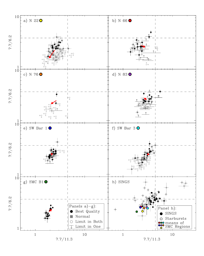
Figure 6.— The 7.7/6.2 ratio versus the 7.7/11.3 ratio. The symbols for each region are indentified in the bottom-right corner of panel g. A value is considered a limit in this plot if either the uncorrected or artifact-corrected spectrum does not have a detection of all bands at $>5\sigma$. In that case, we use the least stringent of the corrected or uncorrected ratios to be conservative. The “best” and “normal” quality points are assigned via visual inspection of the spectra to give some idea of which points are strongly affected by the artifact. The red arrow connects the weighted mean of the uncorrected band ratios to the same value for the corrected ratios. These weighted means are shown also in panel h) with their colors identified by a representative point in each panel a) through g). The dashed line shows the weighted mean values for the SINGS galaxies. Panel h) shows the ratios for the SINGS sample without AGN and the starbursts from Engelbracht et al. (2008).

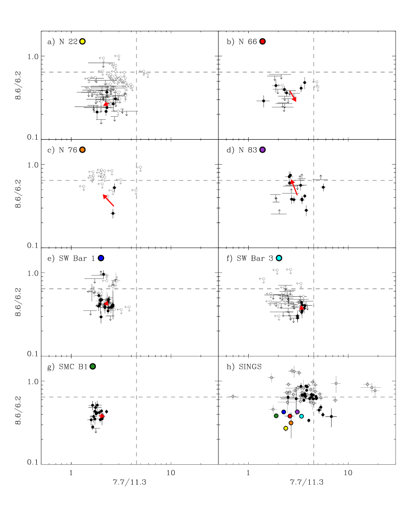
Figure 7.— The 8.6/6.2 ratio versus the 7.7/11.3 ratio. The symbols and annotations in this plot are identical to those in Figure 6.

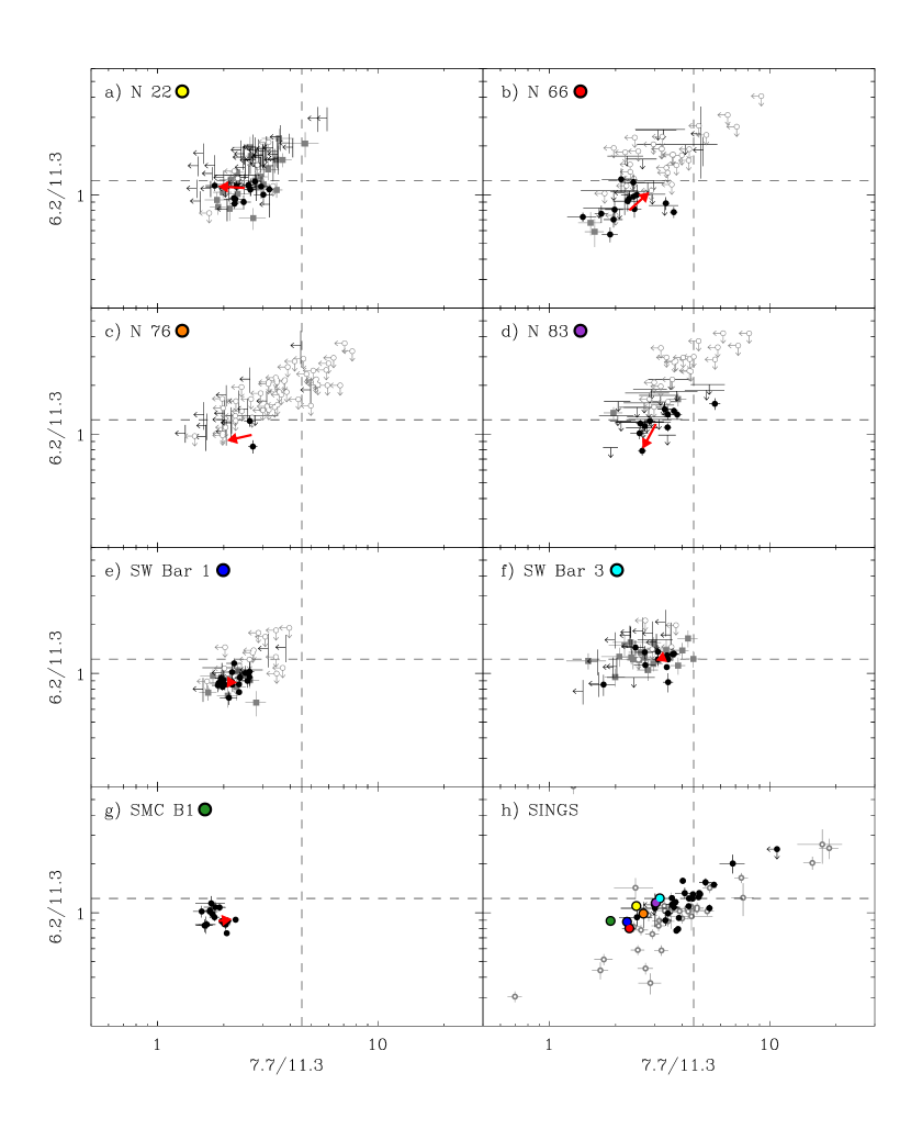
Figure 8.— The 6.2/11.3 ratio versus the 7.7/11.3 ratio. The symbols and annotations in this plot are identical to those in Figure 6.

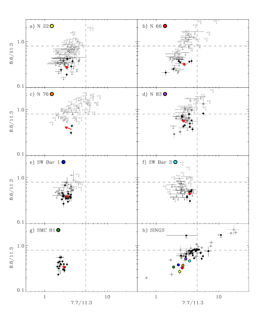
Figure 9.— The 8.6/11.3 ratio versus the 7.7/11.3 ratio. The symbols and annotations in this plot are identical to those in Figure 6.

3.1.2 The 17.0µm Band

In Figures 10 and 11 we show the ratios of the 17.0 µm band to the 7.7 and 11.3 µm bands. Figure 10 shows that the 17.0/11.3 ratio is consistently low in the SMC regions compared to the SINGS mean. Aside from a few outliers, all of the galaxies from SINGS and the starburst samples which cover the same range of 7.7/11.3 have higher ratios of 17.0/11.3. There does not appear to be a clear trend in the 17.0/11.3 vs 7.7/11.3 ratio, particularly since the starburst sample has galaxies with similar 17.0/11.3 ratios but 7.7/11.3 ratios spanning more than an order of magnitude. Because the charge state of the carrier of the 17.0 µm complex is not well-constrained, we also show the ratio of 17.0/7.7 in Figure 11. The region averages of the 17.0/7.7 ratio in the SMC are closer and at times above the SINGS average, spanning a range of $\sim$0.06$-$0.1. We note that for these ratios, the artifact correction has a minimal effect on the results.

Figure 10.— The 17.0/11.3 ratio versus the 7.7/11.3 ratio. The symbols and annotations in this plot are identical to those in Figure 6.

Figure 11.— The 17.0/7.7 ratio versus the 7.7/11.3 ratio. The symbols and annotations in this plot are identical to those in Figure 6.

To summarize, we find that the 17.0/11.3 ratio is low in all SMC regions while the 17.0/7.7 ratio is approximately normal compared to the SINGS sample mean.

3.1.3 Ratios of Individual Bands to the Total PAH Emission

Due to the complexity of comparing among individual bands which may vary independently, we attempt to simplify the comparison by showing the ratio of each band to the total PAH emission. In Figure 12 we show the fraction of the total PAH emission (defined as the sum of the 6.2, 7.7, 8.3, 8.6, 11.3, 12.0, 12.6, 13.6 and 17.0 µm features) carried by each of the major PAH features discussed above. We show the weighted mean of the ratio for all of the spectra in a given region where the relevant feature is detected at $>5\sigma$ in both the original and artifact-corrected version of the spectrum. The large points show the weighted mean for the original data and are connected to a smaller point showing the same weighted mean using the artifact-corrected spectra. We overplot the mean from the SINGS sample (with an error bar showing the standard deviation of the SINGS galaxies) connected with a gray line to guide the eye. We can see from this plot that there are deviations from the SINGS average: 1) the 7.7 micron complex is weaker, 2) the 6.2 and 11.3 µm features are stronger and 3) the 8.6 and 17.0 µm bands are weaker compared to the SINGS average. We note that the conclusion about the weakness of the 17.0 µm complex is enforced by the fact that it is not a major contributor to the total PAH emission, and therefore should be less sensitive to changes in the relative proportion of the flux carried by the 6.2, 7.7, 8.6 and 11.3 µm bands. This agrees with the assertion that the weakness of the 7.7 µm feature drives the relatively normal 17.0/7.7 ratios seen in the SMC.

Figure 12.— The fraction of the total PAH emission carried by each PAH band. The colored points represent the weighted mean of the SMC regions. Small x-axis shifts have been introduced to ensure the points do not overlap. These are connected to a smaller point of the same color to represent the effect of correcting the “dark settle” artifact on the ratio. The SINGS mean is shown in gray connected with a line to guide the eye. The error bar on the SINGS point represents the scatter of the SINGS galaxies, while the error bars on the SMC points show the uncertainty in the weighted mean. Here we omit the 8.3, 12.0, 13.6 and 14.2 µm bands since they make very small contributions to the total PAH emission.

As described in the Introduction, the C-H bands between 11$-$14 µm have the potential to provide information on the structure and hydrogenation of the PAHs. To compare the relative strengths of these bands, we make a plot very similar to Figure 12 but showing the contribution of the 11.3, 12.0, 12.6 and 13.6 µm bands to the total C-H band emission (the sum of the emission in these features). For the SMC regions we can see from this comparison that the 11.3 µm feature carries a similar amount of the total C-H band emission as in the SINGS galaxies, while the 12.6 µm feature carries slightly less and the 12.0 and 13.6 µm features are slightly stronger.

Figure 13.— The fraction of the total C-H PAH emission in the bands between 11$-$14 µm carried by each individual C-H band. The colors and lines are identical to those in Figure 12. The 11.3 feature fraction of the total C-H emission is very similar to that in the SINGS galaxies, in contrast to the 11.3 feature fraction of the total PAH emission, which is higher in the SMC.

3.1.4 Summary of the Band Ratio Results

We have observed clear deviations of the SMC band ratios from the average values found in the SINGS sample:

1. For the three brightest PAH bands at 6.2, 7.7 and 11.3 µm, we find that the 7.7 µm feature is weak compared those at 6.2 and 11.3 µm. The 6.2 µm band is slightly weak compared to the 11.3 µm band.

2. The 8.6 µm feature appears to be weak relative to all of the major bands (6.2, 7.7 and 11.3 µm) and a weaker contributor overall to the total PAH emission.

3. The 17.0 µm feature is weak relative to the 6.2 and 11.3 features. Compared to the SINGS average, however, the 17.0/7.7 ratio is only slightly low. The 17.0 µm feature makes a smaller contribution to the total PAH emission in the SMC than in the SINGS galaxies.

3.2. Band Ratios and Radiation Field Hardness

The ratio of the [Ne III] line at 15.6 µm to the [Ne II] line at 12.8 µm traces the hardness of the radiation field in H II regions (Giveon et al. 2002) and is often used in the context of studying PAH emission because of the prominence of these two lines in the mid-IR (Madden 2000; Smith et al. 2007b; Gordon et al. 2008). It has been suggested that the hardness of the radiation field is the driver of the deficit of PAHs observed at low-metallicity (Madden 2000; Gordon et al. 2008) via enhanced photodissociation of the molecules. In order to understand how the radiation field hardness affects the PAH physical state in the SMC, we show the 7.7/11.3 and 17.0/11.3 ratios as a function of the [Ne III]/[Ne II] ratio in Figures 14 and 15. As will be discussed further in Section 5 these two ratios predominantly trace changes in the ionization and size distribution of PAHs, respectively. We choose these as representative ratios for changes in the PAH physical state. We note that none of the other ratios discussed here show trends with radiation field hardness.

From the ratios shown in these figures, we can see that there is no clear trend in either the 7.7/11.3 or 17.0/11.3 with radiation field hardness. The 7.7/11.3 ratio stays essentially constant to within $\sim 50$% over nearly two orders of magnitude in [Ne III]/[Ne II] ratios. In fact, we have found no clear trends of any band ratio with the [Ne III]/[Ne II] ratio. The same is true for the SINGS galaxies with no AGN, as seen by Smith et al. (2007b). Brandl et al. (2006) similarly found no trend of the 7.7/11.3 ratio over an order-of-magnitude in the neon line ratio for a sample of starburst galaxies observed with IRS on Spitzer. In a resolved study of H II regions in M 101, Gordon et al. (2008) found no correlation between their ionization index (a combination of the neon ratio and the ratio of mid-IR silicon lines) and the 7.7/11.3 ratio, though they do find that the PAH feature equivalent width depends on radiation field hardness. These consistent results across a wide range of physical conditions and metallicity indicate that the radiation field hardness does not have a strong effect on the PAH band ratios.

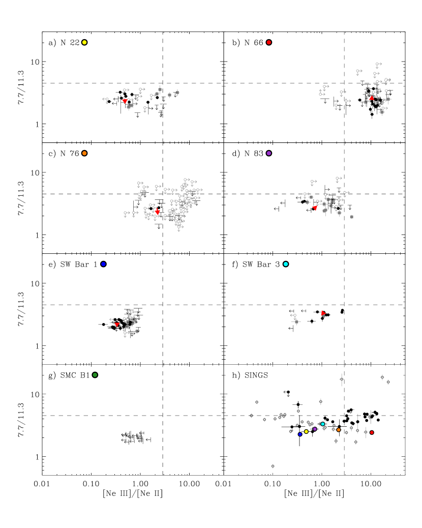
Figure 14.— The 7.7/11.3 ratio versus radiation field hardness as traced by the [Ne III]/[Ne II] ratio. The symbols and annotations in this plot are identical to those in Figure 6. Note that SMC B1 has no detections of either the [Ne III] or [Ne II] line so it does not appear in Panel h.

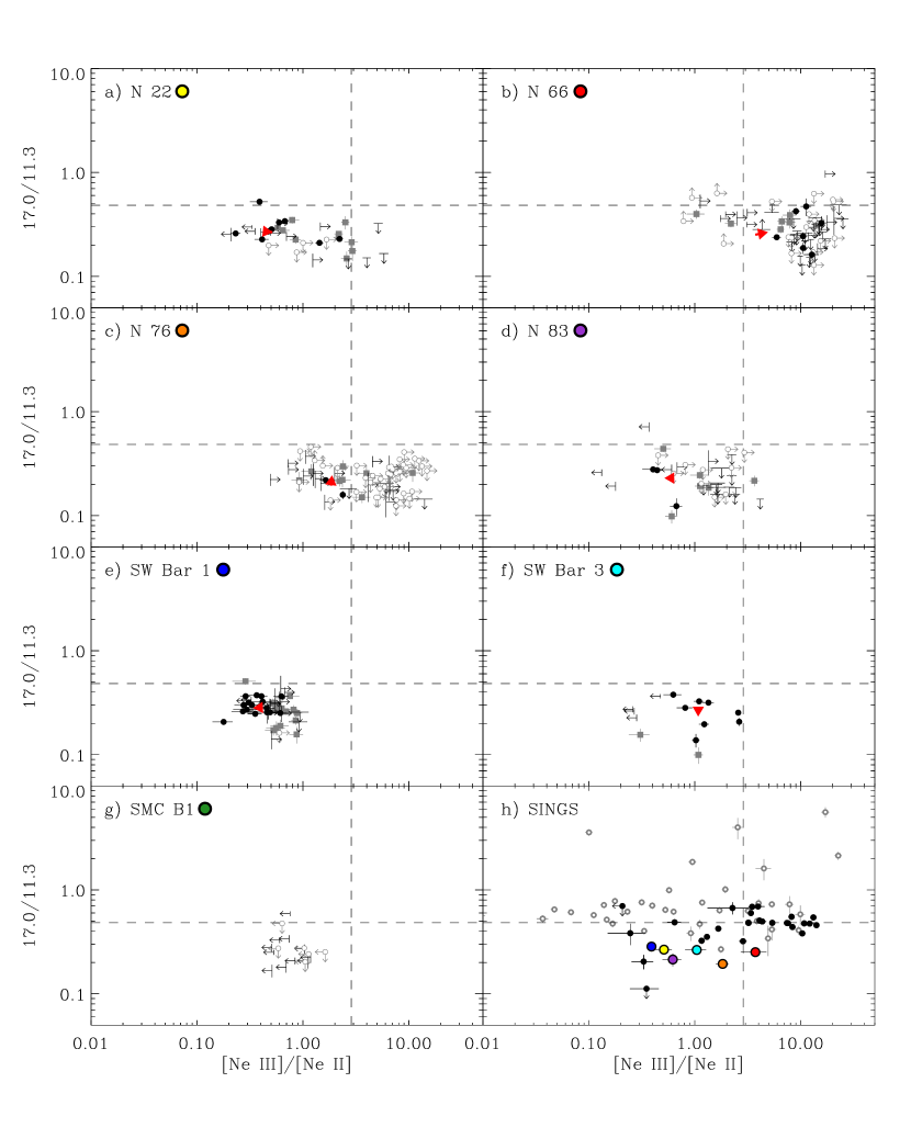
Figure 15.— The 17.0/11.3 ratio versus radiation field hardness as traced by the [Ne III]/[Ne II] ratio. The symbols and annotations in this plot are identical to those in Figure 6. Note that SMC B1 has no detections of either the [Ne III] or [Ne II] line so it does not apper in Panel h.

4. The Physical State of SMC PAHs: Interpreting the Band Ratios

In Section 3, we have enumerated the variations and average properties of the PAH band ratios we observe in the SMC relative to galaxies in the SINGS sample. In the following discussion, we use information gathered from laboratory and theoretical studies to translate the ratios into information about the physical state of the PAHs.

4.1. Interpreting the SMC Results

Our major conclusions about the band ratios in the SMC relative to SINGS are the following: 1) weak 7.7 µm feature relative to the 6.2 and 11.3 µm features, 2) weak 8.6 µm feature relative to all major bands and the total PAH emission and 3) weak 17.0 µm feature relative to the total PAH emission.

We first address conclusion 1), regarding the ratios of the 6.2, 7.7 and 11.3 µm bands. As discussed above, the 6$-$9 µm to 11.3 µm band ratios should simultaneously trace changes in the PAH ionization and size distribution. To aid in interpreting these ratios we use a diagram based on the model of Draine & Li (2001). This model utilizes cross sections for ionized and neutral PAHs as a function of size based on laboratory and theoretical results. The PAHs are exposed to a radiation field with a specified strength and spectral shape and their emission spectrum is calculated. Figure 16 shows the band ratios from Draine & Li (2001) for ionized and neutral PAHs at a range of sizes exposed to radiation fields at 1, 10² and 10⁶ times the Mathis et al. (1983) solar neighborhood radiation field. On this plot we show the band ratios for the SINGS sample with no AGN and the weighted means for the SMC regions. We note that the modeled band ratios shown on this plot are for individual PAHs of a given size, while PAHs in the ISM should have a wide distribution of sizes. Therefore, in comparing the SMC ratios to the models, we use the Draine & Li (2001) results as a guide but not as a way to judge specific PAH sizes.

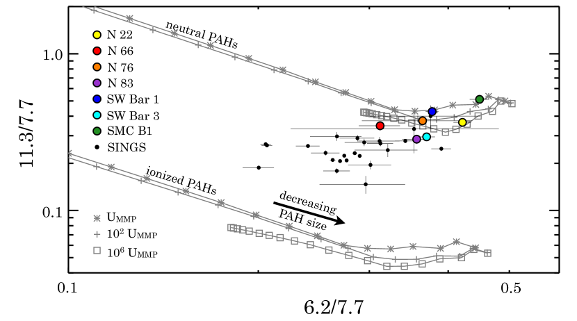
Figure 16.— Model PAH band ratios from Draine & Li (2001) with the SINGS galaxies without AGN overplotted in black and the weighted means of the SMC regions shown in color. The two sets of gray lines show the band ratios for neutral and ionized PAHs and each at three different radiation field strengths (parametrized in units of $\mathrm{U}_{\mathrm{MMP}}$, the solar neighborhood radiation field from Mathis et al. 1983). The SMC regions fall in the area of this diagram compared to the SINGS galaxies that suggests smaller and more neutral PAHs.

The relative locations of the SINGS galaxies and the SMC regions on this plot suggest that SMC PAHs may tend to be smaller and more neutral than those in higher metallicity galaxies. Within the SMC, N 66 falls closest to the SINGS mean, suggesting it has relatively larger and more ionized PAHs. SMC B1, on the other hand, has band ratios which put it at the extreme end of the diagram, suggesting it has the smallest and most neutral PAHs. The spread in the SMC points may be related to the progression of the star-formation happening in the region: SMC B1 is a quiescent molecular region (Rubio et al. 1993; Reach et al. 2000) with abundant molecular gas, but no detectable H II regions while N 66 has a giant H II region with multiple generations of star formation in the vicinity (though it also hosts molecular clouds; Rubio et al. 2000). The remaining regions are intermediate in the star-formation properties but generally seem to follow a trend where more evolved regions like SW Bar 3 and N 83 are consistent with slightly larger and more ionized PAHs while regions such as SW Bar 1 and N 22 tend towards smaller and more neutral PAHs.

It is worthwhile to note that the Draine & Li (2001) model attributes all variation of PAH band strengths to either size or ionization. It is very likely that hydrogenation (in excess of the full aromatic complement of peripheral hydrogens), structure and chemical composition also play a role in determining the band ratios. If there were changes in structure, we would expect to see variations in the relative strengths of the C-H modes. More irregular PAHs should show enhanced emission in the “duo”, “trio” and “quartet” modes as discussed in the Introduction. Under some conditions, PAHs can become super-hydrogenated—with two hydrogen atoms attached to a given carbon atom (Le Page et al. 2003). This edge structure with two hydrogens per carbon is similar to an aliphatic group ($-$CH₂) and is expected to produce similarly aliphatic emission features (Bernstein et al. 1996).

Our observations in the SMC do not show strong evidence for changes in PAH structure (towards more irregular edges) or excess hydrogenation. In Figure 13 we show the fraction of the 11$-$14 µm PAH emission carried by the 11.3, 12.0, 12.6 and 13.6 µm features. We note that in the low-resolution spectra, the 12.6 feature is blended with the [Ne II] line at 12.8 µm. For most regions the 11.3 and 12.0 µm bands carry a similar fraction of the C-H flux as seen in the SINGS sample, however the 13.6 µm feature is enhanced and the 12.6 µm feature is weaker. Changes in structure that produce more emission in “quartet” modes at 13.6 µm would be expected to also enhance “trio” modes at 12.6 µm, as both originate in irregular edges and extensions. Thus, we can not draw a clear conclusion from these band ratios. At the signal-to-noise of our spectra, we do not see clear evidence for any aliphatic features that might result from excess hydrogenation. Clear detection of these features if they exist and higher signal-to-noise measurements of the 13.6 and 14.2 µm bands in the future with JWST will enhance our ability to judge whether SMC PAHs show changes in structure or hydrogen content.

We now move on to conclusions 2) and 3) regarding the weakness of the 8.6 and 17.0 µm features in the SMC. As discussed in the Introduction both 8.6 and 17.0 µm features are expected to arise in large PAHs. Based on theoretical calculations of PAH spectra, the 8.6 µm feature is thought to trace mainly charged PAHs (Bauschlicher et al. 2008). There is no clear identification of the charge state of the 17.0 µm carrier. The weakness of these two features in our spectra provide independent evidence for our interpretation that PAHs in the SMC tend to be smaller and more neutral than their counterparts in more metal rich systems. The particular weakness of the 8.6 µm feature may be due to the combination of size and charge state both favoring less emission in that band.

4.2. Trends of PAH Physical State with Radiation Field Hardness

In Figures 14 and 15 we show the variation of the band ratios as a function of the [Ne III]/[Ne II] ratio. These lines arise in ionized gas and their ratio traces the hardness of the ionizing radiation field. We find no clear evidence for variation of the band ratios with radiation field hardness over nearly two orders of magnitude in the [Ne III]/[Ne II] ratio. PAHs are observed to be depleted in ionized gas (Povich et al. 2007; Lebouteiller et al. 2011) and theoretical studies suggest that the lifetimes of PAHs in ionized gas can be short compared to the H II region lifetimes (Micelotta et al. 2010a). Because of the destruction of PAHs in ionized gas, we may not expect the physical state of the PAHs to strongly depend on the neon line ratio since the PAH emission we observe arises from the PDR around the H II region and is thus physically separate from the gas traced by the neon lines.

4.3. Trends of PAH Physical State with Metallicity

In Figure 17 we show a series of plots illustrating the variation of the several PAH band ratios with metallicity. In general, the SMC occupies a similar region of the plot as other low-metallicity galaxies from the SINGS and starburst samples, though there is considerable scatter. There is a slight trend towards lower 7.7/11.3 ratios as a function of metallicity, though with many outliers. Smith et al. (2007b) found a slight trend for galaxies to show low 17.0/11.3 ratios at lower metallicity. We show their galaxies here, instead using the 17.0/$\Sigma_{PAH}$ as a tracer of the 17.0 µm feature strength that does not depend as heavily on the charge state of the PAHs. The SMC 17.0 µm fraction of the total PAH emission falls below the average for SINGS but above the lowest metallicity SINGS galaxy with detected PAH emission (NGC 2915).

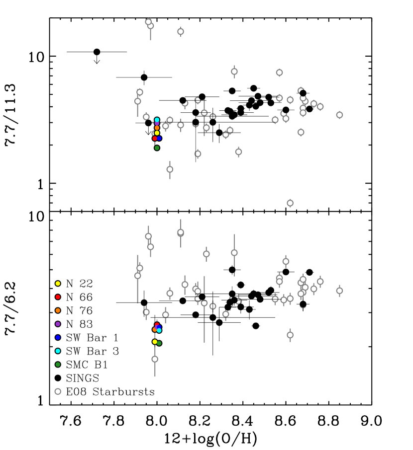
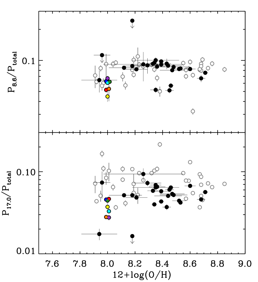
Figure 17.— The band ratios from the SINGS (Smith et al. 2007b), starburst (Engelbracht et al. 2008) and SMC samples versus metallicity. For the SINGS galaxies we use the metallicities for the central regions from Moustakas et al. (2010) using the calibration of Pilyugin & Thuan (2005). The starburst metallicities are T_e based and should be consistent with the Pilyugin & Thuan (2005) results. They are described further in Engelbracht et al. (2008) and do not have uncertainties. We use a metallicity of $12+$log(O/H)$\sim 8.0$ for the SMC (Kurt & Dufour 1998). Small shifts on the x-axis are introduced for the SMC points so they do not overlap.

5. Discussion

5.1. Insights Into the PAH Life-Cycle as a Function of Metallicity

By comparing our measured band ratios with laboratory and theoretical results, we infer that PAHs tend to be smaller on average in the SMC than in higher metallicity galaxies like those represented by the SINGS sample. Note that this is not to say that the SMC is devoid of large PAHs. We do see a clear 17.0 µm feature in our spectra, which requires large PAHs to be present in the ISM at some level. The band ratios suggest that the proportion of large PAHs is decreased relative to small PAHs. If the SMC represents a typical low-metallicity galaxy, we argue that the smaller average PAH sizes have two major implications for the PAH life-cycle at low-metallicity: 1) the change in the size distribution can not be the product of processing in the ISM but must instead reflect changes in PAH formation and 2) the deficit of PAHs in low-metallicity galaxies may be related to the fact that PAHs are formed with smaller average sizes and are therefore more easily destroyed under typical ISM conditions.

5.1.1 Smaller Average PAH Size Due to Formation not Processing

PAHs can be destroyed in many ways: photodissociation (Allain et al. 1996a, b), interactions with energetic particles in hot and/or shocked gas (Micelotta et al. 2010b, a) and interaction with cosmic rays (Micelotta et al. 2011). For all of these processes, our current knowledge of PAH destruction suggests that small PAHs are destroyed more readily than large PAHs. For instance, theoretical models of PAH photodissociation in the diffuse ISM suggest that PAHs with $\lesssim 50$ C atoms are quickly destroyed under typical interstellar conditions (Allain et al. 1996a, b; Le Page et al. 2003) while large PAHs persist longer under the same ISM conditions. Similar trends hold true for processing by shocks, cosmic rays and hot gas (Micelotta et al. 2010b, a, 2011). Therefore, since small PAHs are destroyed more easily than larger PAHs in the ISM, explaining a deficit of large PAHs cannot be the effect of ISM processing unless the destruction process turns large PAHs into small PAHs as a side-effect. Recent studies by Micelotta et al. (2010b) suggest that this is not the case. The dominant destruction mechanism for large PAHs is through interaction with supernova shocks and they find that “daughter” PAHs formed by the fragmentation of the larger grains are very quickly destroyed in the shocked gas. Thus, since small PAHs are destroyed more easily in all ISM processes and they are likely not replenished by the fragmentation of larger PAHs, explaining a deficit of large PAHs cannot be the effect of ISM processing.

We do, however, have ample evidence that processing in the ISM can affect the PAH size distribution in the sense of selectively removing small PAHs. In the vicinity of AGN, multiple studies have shown a decrease in the 6$-$9 µm features relative to the 11.3 µm and longer wavelength features (Smith et al. 2007b; O’Dowd et al. 2009; Diamond-Stanic & Rieke 2010; Wu et al. 2010). Smith et al. (2007b) also found that the 11.3/17.0 ratio decreases in the presence of an AGN, suggesting a stronger contribution from the 17.0 µm feature—a tracer of larger PAHs. These trends suggest that the ISM conditions in the vicinity of the AGN have selectively removed the more fragile, smaller PAHs.

An interesting counterpoint to our study of the SMC is that by Hunt et al. (2010), who presented a study of the PAH band ratios in a sample of blue compact dwarf galaxies (BCDs). These BCDs have particularly intense radiation fields as well as low metallicities and very low dust-to-gas ratios (hence decreased dust shielding). Hunt et al. (2010) found that the band ratios in these galaxies suggested a size distribution shifted towards larger PAHs relative to the galaxies in the SINGS sample (with no AGN), particularly in the strength of the 8.6 µm feature and the low ratios of short-to-long wavelength bands. Because of the low metallicity of these galaxies, we might expect them to show a size distribution shifted towards smaller PAHs, as we have seen in the SMC. It may be the case in these extreme objects that the radiation field is intense enough to remove small PAHs to such a degree that once again larger PAHs dominate the size distribution, regardless of the scarcity of large PAHs. If this were the case, we would expect the abundance of PAHs relative to dust (i.e. the PAH fraction) to be very low in the BCDs. Indeed, Hunt et al. (2010) found that the ratio of PAH emission to the total infrared emission ($\Sigma{\rm PAH}$/TIR), which should trace the PAH fraction, is depressed by more than an order of magnitude on average in these galaxies compared to the SINGS sample.

If processing in the ISM cannot produce the size distribution shifted towards smaller PAHs that we observe, the only other option is that PAHs are formed with smaller sizes in the SMC. Forming PAHs with smaller average sizes in low-metallicity galaxies could be the result of a change with metallicity in the dominant formation mechanisms (i.e. AGB stars, coagulation or chemistry in dense gas—among many other options that have been proposed) and/or a change in the effectiveness of forming large PAHs with the same mechanism. Both of these options are plausible, especially given the simple fact that the raw material that PAHs form out of is less abundant in low-metallicity galaxies, so constructing large PAHs may be inherently more difficult.

5.1.2 Low-Metallicity PAH Deficit as a Consequence of Smaller PAH Sizes

An important consequence of PAHs forming with a distribution shifted towards smaller sizes at low-metallicity is that a larger fraction of PAHs can be destroyed under typical ISM conditions. In general, models of PAH destruction in the ISM find that below a certain PAH size ($\sim 20-50$ C atoms, generally; Le Page et al. 2001, 2003) PAHs are very quickly destroyed. The timescale for destruction of small PAHs is shorter for essentially all destruction mechanisms, as discussed above. With a size distribution shifted to smaller sizes, the quickly destroyed PAHs will represent a larger fraction of the total amount of PAHs. Such a situation may naturally lead to a PAH deficit in low-metallicity galaxies without the need to rely on enhancements in radiation field hardness (Madden 2000; Gordon et al. 2008) or delays between PAH formation in AGB stars versus dust formation in supernovae (Galliano et al. 2008b). We note, however, various mechanisms can be operating simultaneously—i.e. PAHs could be both easier to destroy because of their smaller sizes while also being exposed to harder, more intense radiation fields in low-metallicity galaxies. The interaction of these two effects could contribute to the steepness of the observed drop-off in the PAH fraction below a metallicity of 12$+$log(O/H)$\sim 8.1$ (Engelbracht et al. 2005; Draine et al. 2007).

5.1.3 Relationship of PAH Emission and Radiation Field Hardness

It has been suggested that the deficiency of PAHs in low metallicity galaxies is a product of their destruction by harder and/or more intense radiation fields (see for instance, Madden 2000; Gordon et al. 2008). We have shown that in the SMC the band ratios do not depend strongly on the hardness of the ionizing radiation field, as one might expect if it were instrumental in destroying PAHs. In fact, a wide range of studies have shown no correlation between the radiation field hardness and the band ratios (Brandl et al. 2006; Smith et al. 2007b; Gordon et al. 2008; O’Dowd et al. 2009; Wu et al. 2010), in line with these two tracers probing distinct physical regions (H II region vs. PDR). Some studies do show, however, a correlation of PAH equivalent width with radiation field hardness (e.g. Madden 2000; Beirão et al. 2006; Gordon et al. 2008), such that PAHs have lower equivalent widths in harder radiation fields. This may be the product of the correlation between harder and more intense radiation fields. Young, massive stars capable of creating harder ionizing radiation will also have more intense radiation fields. The intensity of the radiation field may then affect the amount of emission arising in PDRs around the HII region. Meanwhile, the characteristics of the PAH spectrum are determined by conditions within the PDR itself and may be insensitive to the hardness of the ionizing radiation (for a similar argument see Brandl et al. 2006).

5.1.4 Why are SMC PAHs more Neutral?

In addition to being smaller on average than PAHs in the SINGS galaxies, the SMC PAHs also appear to be less ionized. One possible reason for lower levels of ionization may be that PAHs in the SMC are largely confined to dense regions (Sandstrom et al. 2010). The ratio of the ionization to recombination rates should determine the PAH charge and is proportional to $(G_{0}/n_{e})\times\sqrt{T_{gas}}$. If PAHs in the SMC exist in denser regions compared to PAHs at higher metallicity, a decreased ionization level may be a natural consequence. Another reason why PAHs in the SMC may be more neutral is related to their smaller average sizes. Small ionized PAHs may have a shorter lifetime than small neutral PAHs, since ionization in general causes PAHs to be less stable to photodissociation. It is possible that PAHs in the SMC tend to be more neutral because small, ionized PAHs are destroyed even more quickly in the ISM than their neutral counterparts. More detailed PDR modeling including the PAH ionization state may provide insight into why the PAH charge state is different in the SMC than in higher metallicity galaxies.

5.1.5 A Scenario for the PAH Life-Cycle in the SMC

Sandstrom et al. (2010) argued that in the SMC the low mass fraction of dust in PAHs in the diffuse regions compared to the higher fraction in dense regions suggested that PAHs must be forming in dense gas. Their reasoning was that AGB-produced PAHs would primarily be deposited in the diffuse ISM which would then condense to form dense gas, so enhancements of the PAH fraction in dense gas must occur in situ. We propose the following (speculative) scenario to jointly explain the abundance and physical state of SMC PAHs inferred from our study and that of Sandstrom et al. (2010): 1) PAHs are forming in regions of dense gas in the SMC; 2) these PAHs are formed with a smaller average size possibly due to the lower abundance of carbon available in the ISM; 3) as they emerge from dense regions into the diffuse ISM, the PAHs interact with UV photons, shocks and cosmic rays, and a fraction of the PAHs are preferentially destroyed on the small end of the PAH size distribution. In this scenario, a large fraction of the PAHs in the SMC are destroyed in the diffuse ISM, causing a PAH deficit, not necessarily because of harsher conditions, but because the average PAH starts off smaller and thus more “fragile” in the SMC than the average PAH in a higher metallicity galaxy.

6. Summary & Conclusions

We have presented a study of the PAH physical state diagnosed through the ratios of the 6$-$17 µm bands in several regions of the SMC. In comparing our measured band ratios to the SINGS sample, excluding galaxies with AGN, we find several distinct trends: SMC PAHs show a weak 7.7 µm feature relative to the other dominant PAH bands at 6.2 and 11.3 µm and the features at 8.6 and 17.0 µm are weaker contributors to the overall PAH emission. We find no trend of the band ratios as a function of radiation field hardness as traced by the mid-IR [Ne III]/[Ne II] ratio.

Interpreting the band ratios in light of laboratory and theoretical results on the PAH spectrum, we suggest that SMC PAHs are smaller and more neutral than their counterparts in higher metallicity galaxies. Several lines of evidence argue for this interpretation: the 7.7/11.3 and 7.7/6.2 ratio suggests that PAHs are smaller and more neutral based on comparison with the Draine & Li (2001) model and various theoretical and laboratory studies; the 8.6 µm band, which is thought to be dominantly emitted by large, charged PAHs is particularly weak in the SMC; and the 17.0 µm feature—which is thought to arise in skeletal vibrations of large PAHs—is also weak relative to the total PAH emission in the SMC.

We argue that a size distribution shifted towards smaller average sizes can not be the product of ISM processing by UV photons, shocks, cosmic rays or hot gas, since all of those processes more efficiently destroy small PAHs. A variety of literature results suggest that ISM processing creates a size distribution shifted towards larger PAH sizes, the opposite trend we see here. If ISM processing can not create the size distribution we observe, the likely explanation is a change in how PAHs form. This could be a change in the mechanism of PAH formation at low metallicity or a change in the efficiency of creating large PAHs.

Our observations imply that the PAH deficiency at low-metallicities may not be due to enhancements in the hardness or intensity of radiation fields, but rather that PAHs at low-metallicity start off inherently more “fragile” because of their small sizes so a larger proportion of them can be destroyed under typical ISM conditions.

Appendix A Artifacts in the IRS Spectral Mapping and their Mitigation

A.1. Description of the Artifact

In reducing the S⁴MC observations, we found that the spectra were affected by an artifact caused by a time- and positionally variable background level on the detector. This artifact occurred in both SL and LL observations. It appears to be similar to the “dark settle” artifact that can be important for high-resolution observations with IRS. The artifact causes mis-match in the regions where the orders overlap and was first identified because it causes the long wavelength end of SL2 and the short wavelength end of SL1 to be offset from each other, sometimes significantly. Since this wavelength region covers the 7.7 µm PAH feature, understanding the effects of this artifact was crucial for our study. In Figure 18 we show several spectra from the SW Bar 1 region illustrating the mismatches at SL and LL caused by the artifact. Similar effects are seen in all maps, except for the deep SMC B1 #1 SL map, which used 60 second ramps and does not appear to suffer from this artifact.

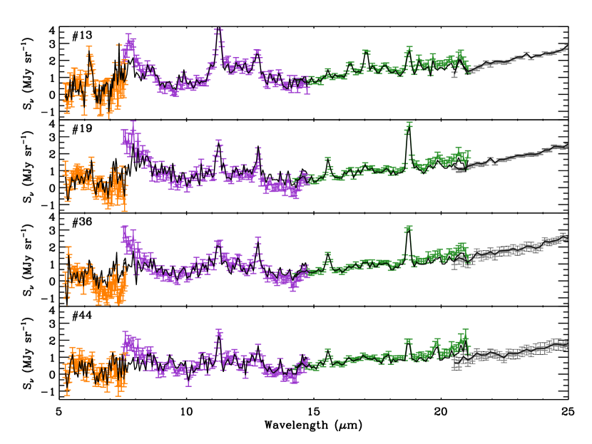
Figure 18.— Several spectra from the map of SW Bar 1 illustrating various degrees of mis-match at the SL2/SL1 and LL2/LL1 overlap regions. The uncorrected orders are shown in color—SL2 in orange, the SL1 in purple, the LL2 in green and the LL1 order in gray. The offsets in the overlap regions are due to a time- and positionally varying dark level on the detector. The black spectrum overlayed shows these same regions after the correction described in this Appendix. The correction derived from the inter-order regions greatly improves the mis-match at the SL2/SL1 overlap, but it may oversubtract real 7.7 µm PAH emission.

We found that the shape and magnitude of the offsets can generally be explained by residual background emission that is apparent in the inter-order region of the BCDs. The residuals persists after removal of the “off” observations and are much larger in magnitude than the difference in zodiacal light or MW foreground between the map position and the “off” position. The average properties of this dark level can be seen in the median background-subtracted BCD for each mapping AOR—created by subtracting the median background image (created in CUBISM) from each of the BCDs in a mapping AOR and then combining the stack of all of the BCDs to generate one median background-subtracted BCD. Figure 19 shows these for each of our SL mapping observations and Figure 20 shows these for each of our LL mapping observations. In these Figures we have masked out the orders and the peak-up arrays to show the residual background more clearly.

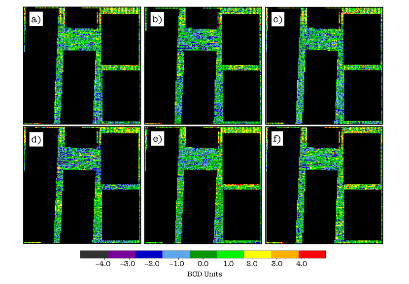
Figure 19.— The median of all background subtracted BCDs for the SL mapping AORs in a) N22 North, b) N66 North, c) N 76 #1, d) N 83, e) SW Bar 1 and f) SW Bar 3. The SL1, SL2 and SL3 orders and the peak-up arrays have been masked to more clearly show the background structure. These images highlight the non-time variable characteristics of the residual background, which are similar in each mapping AOR. These include a higher background level at the top of the detector ($\sim$8 µm in the SL1 order and SL3) and in the middle of the detector (at $\sim$ 5-6 µm in the SL2 and $\sim$ 12 µm in SL1).

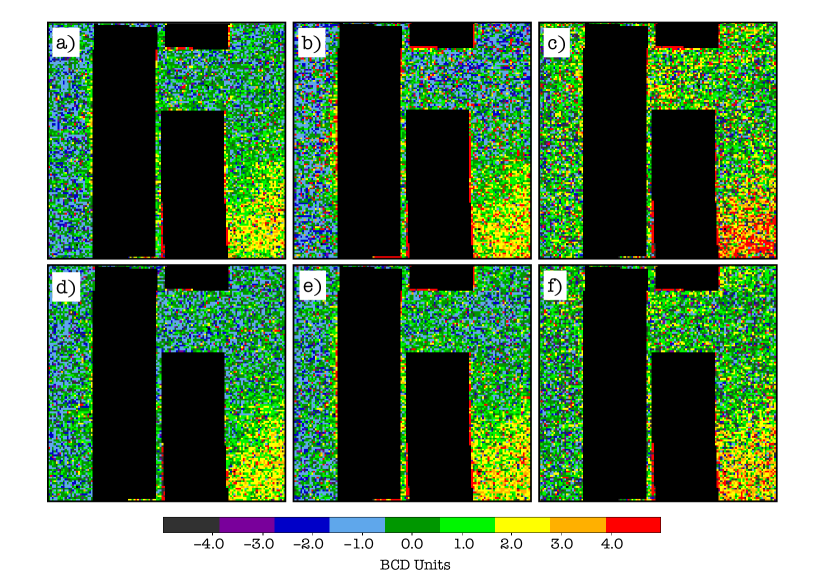
Figure 20.— The median of all background subtracted BCDs for the LL mapping AORs in a) N22, b) N66, c) N76, d) N83, e) SW Bar 1 and f) SW Bar 3. The LL1, LL2 and LL3 orders have been masked out to show the residual background more clearly. These images highlight the non-time variable characteristics of the residual background. For the LL maps, the residual background is concentrated in the bottom right of the detector. This causes an offset at the long wavelength end of LL2, which can be seen for SW Bar 1 in Figure 18 when the LL2 and LL1 orders do not agree in their overlap region.

In addition to the spatial structure of the background, there is also some degree of time-variability. In Figure 21 we illustrate the time variations of the residual background by displaying the median of a $\sim$5 pixel wide strip of the background subtracted BCDs versus BCD number (essentially a time sequence of the observations).

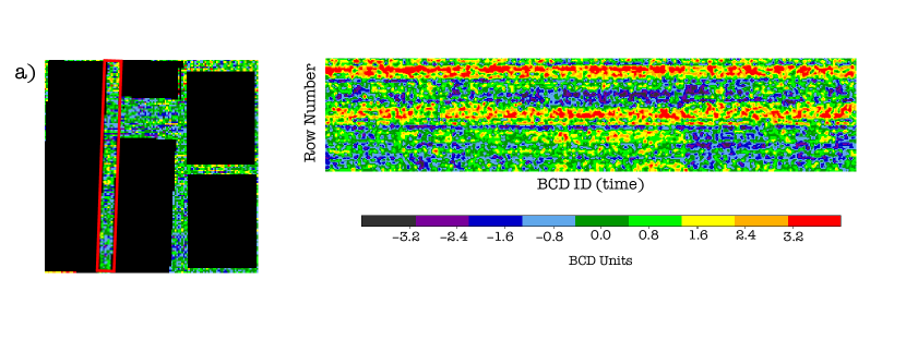
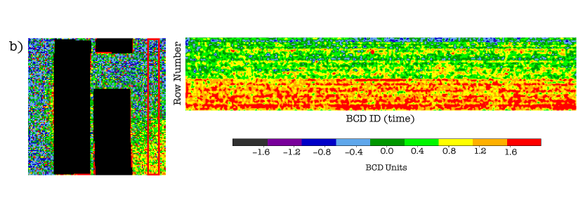
Figure 21.— The median value of the background subtracted BCD in a $\sim$5 pixel wide box (overlayed in red on the median BCD on the left) as a function of BCD number, which generally corresponds to time in the AOR. Panel a) shows the N66 South SL mapping AOR that includes 600 BCDs and panel b) shows the N 66 LL mapping AOR that includes 686 BCDs. The images have been smoothed with a 3$\times$3 pixel Gaussian to suppress noise. These images highlight the time-variable characteristics of the residual background level.

A.2. Correction of the Artifact Derived from Inter-order Background Level

To correct the effects of the artifact, we use the inter-order regions to determine the spatial shape and time-variability of the residual background. This approach is very similar to that done by Starkey et al. (2011, in prep). Because of pixel-based noise, we generally need to average BCDs together as a function of time to improve our determination of the background. At SL wavelengths the presence of the “peak up” arrays on the right-side of the BCD make the available inter-order regions very small, since scattered light from the peak up arrays affects the nearby inter-order regions. We are therefore limited to the small strip between the SL1 and SL2/SL3 orders to characterize the vertical spatial dependence of the residual background (this region is highlighted in Figure 21). For the SL orders we determine the median BCD value as a function of time and vertical row in a box $\sim$5 pixels wide by 11 pixels high by 3 BCDs long. We then create a correction image for each BCD where all columns contains this median. Finally, we apply the SL flatfield to get the appropriate value within the orders.

At LL wavelengths, the lack of peak up arrays make this process much simpler. In addition, there is far less time variability in the LL residual background so we use a simpler correction derived from the median BCDs shown in Figure 20. We mask the LL orders and fit a horizontal polynomial to each row of the BCD, filling in each row of the correction image with this fit. We then apply a vertical polynomial smoothing in a 10 pixel box and finally use the LL flatfield image to obtain the correction in the LL orders. For both the SL and LL we subtract these correction images from the original BCDs.

The effect of the correction on several spectra can be seen in Figure 18 in black. The agreement between orders in the overlap region is essentially always improved after the correction. Most of this correction comes from removing flux in the 7$-$8 µm region, coincident with the 7.7 PAH feature. Because of the limited information about the spatial structure of the residual background and the large effect it has on the PAH feature, we use both the corrected and uncorrected spectra to analyze the PAH band ratios in this paper. Future work my reveal the source of this residual background and improve our determination of the PAH feature strengths.

To conclude we make a few remarks about the sort of observations this artifact is likely to affect. Generally, the residual background level is not an issue in typical IRS observations when either (1) an in-slit background can be subtracted, as in the case of point source observations; (2) the background observation is very close in time to the mapping observation, for example when a “nod” position can be used for background subtraction; or (3) when the object being mapped is bright enough that these low-level variations are negligible. In the SMC we are observing faint emission using the full IRS slit and our “off” observation occurs after $\sim$600 pointings. Thus, the S⁴MC observations present a somewhat unique situation where the residual background artifacts are important to remove.

Facilities: Spitzer ()

References

- Allain et al. (1996a) Allain, T., Leach, S., & Sedlmayr, E. 1996a, A&A, 305, 602
- Allain et al. (1996b) —. 1996b, A&A, 305, 616
- Allamandola et al. (1985) Allamandola, L. J., Tielens, A. G. G. M., & Barker, J. R. 1985, ApJ, 290, L25
- Allamandola et al. (1989) —. 1989, ApJS, 71, 733
- Bakes & Tielens (1994) Bakes, E. L. O., & Tielens, A. G. G. M. 1994, ApJ, 427, 822
- Bakes & Tielens (1998) —. 1998, ApJ, 499, 258
- Bauschlicher et al. (2009) Bauschlicher, C. W., Peeters, E., & Allamandola, L. J. 2009, ApJ, 697, 311
- Bauschlicher et al. (2008) Bauschlicher, Jr., C. W., Peeters, E., & Allamandola, L. J. 2008, ApJ, 678, 316
- Beirão et al. (2006) Beirão, P., Brandl, B. R., Devost et al., 2006, ApJ, 643, L1
- Berné et al. (2007) Berné, O., Joblin, C., Deville, Y., et al., 2007, A&A, 469, 575
- Bernstein et al. (1996) Bernstein, M. P., Sandford, S. A., & Allamandola, L. J. 1996, ApJ, 472, L127
- Bolatto et al. (2007) Bolatto, A. D., Simon, J. D., Stanimirović, S., et al., 2007, ApJ, 655, 212
- Boulanger et al. (1996) Boulanger, F., Abergel, A., Bernard, J.-P., et al., 1996, A&A, 312, 256
- Brandl et al. (2006) Brandl, B. R., Bernard-Salas, J., Spoon, H. W. W., et al., 2006, ApJ, 653, 1129
- Contursi et al. (2000) Contursi, A., Lequeux, J., Cesarsky, D., et al., 2000, A&A, 362, 310
- Diamond-Stanic & Rieke (2010) Diamond-Stanic, A. M., & Rieke, G. H. 2010, ApJ, 724, 140
- Draine & Li (2001) Draine, B. T., & Li, A. 2001, ApJ, 551, 807
- Draine & Li (2007) —. 2007, ApJ, 657, 810
- Draine et al. (2007) Draine, B. T., Dale, D. A., Bendo, G. et al., 2007, ApJ, 663, 866
- Engelbracht et al. (2005) Engelbracht, C. W., Gordon, K. D., Rieke, G. H., et al., 2005, ApJ, 628, L29
- Engelbracht et al. (2008) Engelbracht, C. W., Rieke, G. H., Gordon, K. D., et al., 2008, ApJ, 678, 804
- Galliano et al. (2008a) Galliano, F., Dwek, E., & Chanial, P. 2008a, ApJ, 672, 214
- Galliano et al. (2008b) Galliano, F., Madden, S. C., Tielens, A. G. G. M., Peeters, E., & Jones, A. P. 2008b, ApJ, 679, 310
- Giveon et al. (2002) Giveon, U., Sternberg, A., Lutz, D., Feuchtgruber, H., & Pauldrach, A. W. A. 2002, ApJ, 566, 880
- Gordon et al. (2008) Gordon, K. D., Engelbracht, C. W., Rieke, G. H., et al., 2008, ApJ, 682, 336
- Helou et al. (2000) Helou, G., Lu, N. Y., Werner, M. W., Malhotra, S., & Silbermann, N. 2000, ApJ, 532, L21
- Helou et al. (2001) Helou, G., Malhotra, S., Hollenbach, D. J., Dale, D. A., & Contursi, A. 2001, ApJ, 548, L73
- Hilditch et al. (2005) Hilditch, R. W., Howarth, I. D., & Harries, T. J. 2005, MNRAS, 357, 304
- Hollenbach & Tielens (1999) Hollenbach, D. J., & Tielens, A. G. G. M. 1999, Reviews of Modern Physics, 71, 173
- Hony et al. (2001) Hony, S., Van Kerckhoven, C., Peeters, E., et al., 2001, A&A, 370, 1030
- Hudgins et al. (1994) Hudgins, D. M., Sandford, S. A., & Allamandola, L. J. 1994, J. Phys. Chem., 98, 4243
- Hunt et al. (2010) Hunt, L. K., Thuan, T. X., Izotov, Y. I., & Sauvage, M. 2010, ApJ, 712, 164
- Kelsall et al. (1998) Kelsall, T., Weiland, J. L., Franz, B. A., et al., 1998, ApJ, 508, 44
- Kurt & Dufour (1998) Kurt, C. M., & Dufour, R. J. 1998, in Revista Mexicana de Astronomia y Astrofisica Conference Series, Vol. 7, Revista Mexicana de Astronomia y Astrofisica Conference Series, ed. R. J. Dufour & S. Torres-Peimbert, 202–+
- Le Page et al. (2001) Le Page, V., Snow, T. P., & Bierbaum, V. M. 2001, ApJS, 132, 233
- Le Page et al. (2003) —. 2003, ApJ, 584, 316
- Lebouteiller et al. (2011) Lebouteiller, V., Bernard-Salas, J., Whelan, D. G., et al., 2011, ApJ, 728, 45
- Lee et al. (2009) Lee, M.-Y., Stanimirović, S., Ott, J., et al., 2009, AJ, 138, 1101
- Léger & Puget (1984) Léger, A., & Puget, J. L. 1984, A&A, 137, L5
- Leroy et al. (2009) Leroy, A. K., Bolatto, A., Bot, C., et al., 2009, ApJ, 702, 352
- Li & Draine (2002) Li, A., & Draine, B. T. 2002, ApJ, 576, 762
- Madden (2000) Madden, S. C. 2000, New Astronomy Review, 44, 249
- Madden et al. (2006) Madden, S. C., Galliano, F., Jones, A. P., & Sauvage, M. 2006, A&A, 446, 877
- Massey et al. (1989) Massey, P., Parker, J. W., & Garmany, C. D. 1989, AJ, 98, 1305
- Mathis et al. (1983) Mathis, J. S., Mezger, P. G., & Panagia, N. 1983, A&A, 128, 212
- Micelotta et al. (2010a) Micelotta, E. R., Jones, A. P., & Tielens, A. G. G. M. 2010a, A&A, 510, A37
- Micelotta et al. (2010b) —. 2010b, A&A, 510, A36
- Micelotta et al. (2011) —. 2011, A&A, 526, A52
- Moustakas et al. (2010) Moustakas, J., Kennicutt, Jr., R. C., Tremonti, et al., 2010, ApJS, 190, 233
- Moutou et al. (2000) Moutou, C., Verstraete, L., Léger, A., Sellgren, K., & Schmidt, W. 2000, A&A, 354, L17
- O’Dowd et al. (2009) O’Dowd, M. J., Schiminovich, D., Johnson, B. D., et al., 2009, ApJ, 705, 885
- O’Halloran et al. (2006) O’Halloran, B., Satyapal, S., & Dudik, R. P. 2006, ApJ, 641, 795
- Peeters et al. (2002) Peeters, E., Hony, S., Van Kerckhoven, et al., 2002, A&A, 390, 1089
- Peeters et al. (2004) Peeters, E., Mattioda, A. L., Hudgins, D. M., & Allamandola, L. J. 2004, ApJ, 617, L65
- Pilyugin & Thuan (2005) Pilyugin, L. S., & Thuan, T. X. 2005, ApJ, 631, 231
- Povich et al. (2007) Povich, M. S., Stone, J. M., Churchwell, E., et al., 2007, ApJ, 660, 346
- Rapacioli et al. (2005) Rapacioli, M., Joblin, C., & Boissel, P. 2005, A&A, 429, 193
- Reach et al. (2000) Reach, W. T., Boulanger, F., Contursi, A., & Lequeux, J. 2000, A&A, 361, 895
- Rubio et al. (2000) Rubio, M., Contursi, A., Lequeux, J., et al., 2000, A&A, 359, 1139
- Rubio et al. (1993) Rubio, M., Lequeux, J., Boulanger, F., et al., 1993, A&A, 271, 1
- Sandstrom et al. (2010) Sandstrom, K. M., Bolatto, A. D., Draine, B. T., Bot, C., & Stanimirović, S. 2010, ApJ, 715, 701
- Sandstrom et al. (2009) Sandstrom, K. M., Bolatto, A. D., Stanimirović, S., van Loon, J. T., & Smith, J. D. T. 2009, ApJ, 696, 2138
- Schutte et al. (1993) Schutte, W. A., Tielens, A. G. G. M., & Allamandola, L. J. 1993, ApJ, 415, 397
- Smith et al. (2007a) Smith, J. D. T., Armus, L., Dale, D. A., et al., 2007a, PASP, 119, 1133
- Smith et al. (2007b) Smith, J. D. T., Draine, B. T., Dale, D. A., et al., 2007b, ApJ, 656, 770
- Stanimirović et al. (2005) Stanimirović, S., Bolatto, A. D., Sandstrom, K., et al., 2005, ApJ, 632, L103
- Szczepanski & Vala (1993) Szczepanski, J., & Vala, M. 1993, Nature, 363, 699
- Tielens (2008) Tielens, A. G. G. M. 2008, ARA&A, 46, 289
- Wakelam & Herbst (2008) Wakelam, V., & Herbst, E. 2008, ApJ, 680, 371
- Wolfire et al. (1995) Wolfire, M. G., Hollenbach, D., McKee, C. F., Tielens, A. G. G. M., & Bakes, E. L. O. 1995, ApJ, 443, 152
- Wolfire et al. (2008) Wolfire, M. G., Tielens, A. G. G. M., Hollenbach, D., & Kaufman, M. J. 2008, ApJ, 680, 384
- Wu et al. (2006) Wu, Y., Charmandaris, V., Hao, L., et al., 2006, ApJ, 639, 157
- Wu et al. (2010) Wu, Y., et al. 2010, ApJ, 723, 895