X-Shooter GTO: Chemical analysis of a sample of EMP candidates

Abstract

Context. Extremely metal-poor stars (EMP) are very rare objects that hold in their atmospheres the fossil record of the chemical composition of the early phases of Galactic evolution. Finding these objects and determining their chemical composition provides important constraints on these early phases.

Aims. Using a carefully designed selection method, we chose a sample of candidate EMP stars from the low resolution spectra of the Sloan Digital Sky Survey and observed them with X-Shooter at the VLT to confirm their metallicities and determine abundances for as many elements as possible.

Methods. The X-Shooter spectra are analysed by means of one-dimensional, plane-parallel, hydrostatic model atmospheres. Corrections for the granulation effects are computed using CO5BOLD hydrodynamical simulations.

Results. All the candidates are confirmed to be EMP stars, proving the efficiency of our selection method within about 0.5 dex. The chemical composition of this sample is compatible with those of brighter samples, suggesting that the stars in the Galactic halo are well mixed.

Conclusions. These observations show that it is feasible to observe, in a limited amount of time, a large sample of about one hundred stars among EMP candidates selected from the SDSS. Such a size of sample will allow us, in particular, to confirm or refute the existence of a vertical drop in the Galactic Halo metallicity distribution function around [Fe/H]$\sim-3.5$.

1 Introduction

Stellar data show that the Galaxy, after the Big Bang, was very rapidly enriched in elements heavier than Li by the ejecta of the first stars. The stars observable nowadays are more or less metal-rich because they formed from material more or less enriched in heavy elements. Low mass stars (${\rm M}<0.8{\rm M}_{\odot}$), have mean-sequence lifetimes older than the age of the Universe and, if they formed at the beginning of the Universe, before significant metal enrichment took place, they would still shine today and could be observable. It is nevertheless difficult to find these rare extremely metal-poor stars, which are the relics of the earliest phases of the Galactic evolution. Dedicated surveys have been designed (the most relevant being Beers et al. 1985, 1992; Beers 1999 and Christlieb et al. 2008 but the earlier surveys of Bond 1970; Slettebak & Brundage 1971; Bidelman & MacConnell 1973, are also relevant), with some striking (Bessell & Norris 1984; Molaro & Castelli 1990; Molaro & Bonifacio 1990; Christlieb et al. 2002; Frebel et al. 2005; Norris et al. 2007), but limited successes, owing to the rarity of these stars. The number of extremely metal-poor stars is small, and their study has raised some questions, because in many of them the carbon abundance exceeds by more than two orders of magnitude the value expected if they had a solar-scaled composition (Christlieb et al. 2002; Frebel et al. 2005; Norris et al. 2007): as a consequence, the global metallicity of these objects is comparable to that of a typical metal-poor star of about [Fe/H]=-2.5.

One way to extend the sample is to use surveys of greater sky coverage, at the cost of handling large quantities of data. Another solution is to extend the surveys to fainter magnitudes, which means the exploration of a larger volume, finding more remote faint targets. With a strategy of combining adapted sophisticated criteria for target selection and high-efficiency spectrographs for the high-resolution follow-up (X-Shooter), a few more extremely metal-poor stars should be found. This is what we tried with the SDSS data for the target selection, and we present here the results. We took the opportunity of the French-Italian X-Shooter guaranteed time observations (GTOs) to observe a sample of good candidates of turn-off, extremely metal-poor (EMP) stars. The high efficiency of X-Shooter permits us to observe in about one hour a 16-17 mag star, during one night between four and eight stars can be observed.

2 Target selection

The Sloan Digital Sky Survey (SDSS, York et al. 2000) archive is a real treasure chest when searching for rare objects, which we have exploited in the past five years in our quest to identify extremely metal-poor candidates. The survey is optimised to observe galaxies, but many stars are in the sample of observed objects. SDSS provides photometry in five broad bands specifically tied to extragalactic surveys: $u$ centred at 355.1 nm, $g$ at 468.6 nm, $r$ at 615.5 nm, $i$ at 748.1 nm, and $z$ at 893.1 nm. We used the $(g-z)_{0}$ colour to derive the effective temperature of the stars (Ludwig et al. 2008). For a subsample of objects, a wide range spectrum (380-920 nm) is provided, at low resolution (R=1800-2000), and low signal-to-noise ratio (hereafter S/N) of about 20 at 400 nm for a $g=17$ object. We selected objects classified as stars in the SDSS archive, with both photometric and spectroscopic observations available and turn-off star colours. In this way, we were able to fix the gravity at 4.0 on a logarithmic scale (c.g.s. units). The sample of about 125 000 spectra obtained from this selection was analysed with an automatic procedure, to derive the metallicity of the stars. We inspected by eye all the spectra that were found to be more metal-poor than $\left[{\rm Fe/H}\right]=-2.5$, in order to select the most promising candidates. Eight of these candidates were observed during the French-Italian guaranteed time observation (GTO) of the X-Shooter spectrograph at VLT. Two of them were observed in April and May 2010 (Bonifacio et al. 2011a), and six in February 2011. One of the candidates observed in the last run appears particularly interesting, showing no iron line in the X-Shooter spectrum. A dedicated paper on this star is in preparation. For the selection of the candidates presented in this work, taking into account the target coordinates, only about 40 000 objects, out of the sample of 125 000, were observable, and 754 of them have a metallicity that is lower than $\left[{\rm Fe/H}\right]\leq-3.5$. These numbers tell us that extremely-metal-poor stars might not be so rare as generally assumed, and that a systematic programme to observe them could significantly extend the number of these primitive stars detected.

3 Observations and data reduction

The observations were performed on the night of 10 February 2011 with Kueyen (VLT UT2) and the high efficiency spectrograph X-Shooter (D’Odorico et al. 2006). In Table 1, we present the coordinates and some basic photometric informations about the programme stars. The log of the observation is presented in Table 2. The X-Shooter spectra range from 300 nm to 2400 nm and gathered by three detectors. The observations have been performed in staring mode with $1\times 2$ on-chip binning along the spectral direction and with the integral field unit (IFU), which re-images an input field of 4”x 1.8” into a pseudo slit of 12”x 0$\aas@@fstack{\prime\prime}$6 (Guinouard et al. 2006). As no spatial information was reachable for our targets, the aim of using the IFU was to use it as a slicer with three 0$\aas@@fstack{\prime\prime}$6 slices. This corresponds to a resolution of R=7900 in the UVB arm and R=12600 in the VIS arm. The spectra were reduced using the X-Shooter pipeline (Goldoni et al. 2006), which performs the bias and background subtraction, cosmic ray hit removal (Van Dokkum 2001), sky subtraction (Kelson 2003), flat-fielding, order extraction, and merging. However, the spectra were not reduced using the IFU pipeline recipes. Each of the three slices of the spectra were instead reduced separately in slit mode with a manual localisation of the source and the sky. This method allowed us to perform an optimal extraction of the spectra leading to an efficient cleaning of the remaining cosmic ray hits but also to a noticeable improvement in the S/N.

Table 1: Coordinates and photometric data.

SDSS ID	RA	Dec	$u$	$g$	$r$	$i$	$z$	J	H	K	AV
	J2000.0	J2000.0	[mag]	[mag]	[mag]	[mag]	[mag]	[mag]	[mag]	[mag]
J044638-065529	04  46  38.234	$-$06  55  29.07	$19.454$	$18.592$	$18.224$	$18.102$	$18.001$	$-$	$-$	$-$	$0.354$
J082511+163459	08  25  11.458	+16  34  59.97	$18.622$	$17.563$	$17.089$	$16.875$	$16.774$	$16.048$	$15.349$	$15.359$	$0.142$
J085211+033945	08  52  11.519	+03  39  45.15	$17.834$	$16.906$	$16.646$	$16.534$	$16.492$	$15.765$	$15.301$	$15.355$	$0.184$
J090733+024608	09  07  33.285	+02  46  08.17	$17.277$	$16.329$	$16.010$	$15.869$	$15.826$	$15.005$	$14.642$	$14.784$	$0.095$
J133718+074536	13  37  18.760	+07  45  36.31	$19.181$	$18.277$	$18.041$	$17.957$	$17.923$	$-$	$-$	$-$	$0.118$

Optical magnitudes are from SDSS, infrared magnitudes from 2MASS.

Table 2: Log of the observations.

Star	date	Exp Time (sec)	mode	S/N @ 650 nm	SDSS Obj. Typea
SDSS J044638-065528	2011-02-12	5400	IFU	110	Ser BLUE
SDSS J082511+163459	2011-02-12	5400	IFU	130	RED STD
SDSS J085211+033945	2011-02-12	3600	IFU	150	SP STD
SDSS J090733+024608	2011-02-12	1800	IFU	120	SP STD
SDSS J133718+074536	2011-02-12	3450	IFU	80	RED STD
a Object type, based on colours that motivated the selection of this object for SDSS spectroscopy:
SP STD = spectrophotometric standard; Ser BLUE = serendipity blue object; RED STD = reddening standard.

The use of the IFU can cause some problems with the sky subtraction because there is only $\pm 1$ arcsec on both sides of the object. In the case of a large gradient in the spectral flux (caused by emission lines), the modelling of the sky background signal can be of poor quality owing to the small number of points used in the modelling.

4 Model atmospheres

The analysis was done with 1D, plane-parallel, hydrostatic model atmospheres, computed in local thermodynamical equilibrium (hereafter LTE) with ATLAS 9 (Kurucz 1993, 2005) in its Linux version (Sbordone et al. 2004; Sbordone 2005), line opacity being treated using opacity distribution functions (ODFs). We used the ODFs computed by Castelli & Kurucz (2003), with a microturbulent velocity of 1$\mathrm{km\,s^{-1}}$. Convection was treated in the mixing length approximation with $\alpha_{\mathrm{MLT}}$=1.25 and the overshooting option in ATLAS was switched off. For each star, we computed an ATLAS 9 model, with the parameters derived from the photometry. For the abundance corrections related to thermal inhomogeneities and differences in stratification (3D corrections hereafter), we used the 3D-CO⁵BOLD model (Freytag, Steffen, & Dorch 2002; Freytag et al. 2011) with the closest parameters in the CIFIST grid (see Ludwig et al. 2009) and the associated $\mathrm{1D}_{\mathrm{LHD}}$ model (Caffau & Ludwig 2007) as reference.

5 Analysis

The effective temperature was derived from the photometry ($g-z$ colour), by using the calibration described in Ludwig et al. (2008). We also fitted the wings of the H$\alpha$ line with a grid of synthetic profiles computed using ATLAS models and a modified version of the BALMER code, which uses the theory of Barklem et al. (2000, 2000b) for the self-broadening and the profiles of Stehlé & Hutcheon (1999) for Stark broadening. For three stars of our sample (SDSS J044638-065528, SDSS J085211+033945, and SDSS J133718+074536), we find a good consistency of ${\rm T_{\rm eff}}$ from the H$\alpha$ and photometry, to within 100 K. SDSS J090733+024608 displays an H$\alpha$ fitting temperature cooler than the photometric one by about 300K, while SDSS J082511+163459 is 500 K cooler. In this latter star, the red wing of H$\alpha$ in the observed spectrum is affected by an absorption that could explain, at least in part, the disagreement between the effective temperature derived from the H$\alpha$ fitting profile and from photometry. We decided to keep a coherent effective temperature and our choice was the photometric one because we consider this to be more robust. X-Shooter is an echelle spectrograph, and the continuum placement in the H$\alpha$ region, which greatly affects the temperature determination, cannot be easily performed in an objective way. For the gravity, we assumed for all the stars that $\log g=4.0$, because the stars are selected from the colours to be at the turn-off. X-Shooter spectra do not provide us with many possibilities to derive the gravity. For three stars, some Fe ii lines are detectable, and the comparison of the iron abundance from the two ionization states can be used as a check of the gravity. For one of them (SDSS J082511+163459) the agreement is good, considering to the quality of the data (0.11 dex). For SDSS J085211+033945 and SDSS J090733+024608, the difference is non-negligible, 0.33 and 0.27 dex, respectively, but the two Fe ii lines visible in the X-Shooter spectra are very weak and give a difference in abundance of 0.15 and 0.14 dex, respectively.

Owing to the “low” resolution of the X-Shooter spectra we were unable to derive the abundance from weak lines, nor derive the micro-turbulence directly from the abundance versus (vs.) equivalent width (EW) relation, which we derived instead using the formula in Edvardsson et al. (1993). A change in the microturbulence of $\Delta\xi=0.5$$\mathrm{km\,s^{-1}}$ induces a change in the iron abundance of $\Delta\left[{\rm Fe/H}\right]\sim 0.15$ dex. For the same reason, we were unable to detect several elements. The solar abundances that we used was this from Caffau et al. (2011a) for Fe, and those from Lodders et al. (2009) for the other elements. The atomic parameters adopted for the spectral-synthesis fitting are from the “First Stars” survey (Bonifacio et al. 2009; Cayrel et al. 2004; François et al. 2007). In Fig. 1, the observed spectra of the five stars of the sample are shown in the range of the K and H-Ca ii lines.

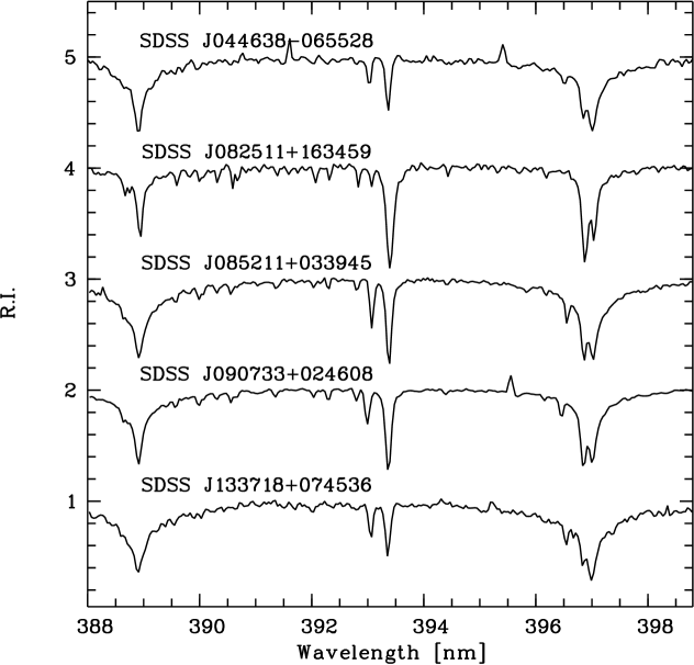
Figure 1: The X-Shooter observed spectra, in the range of the K and H-Ca ii lines for the five stars of the sample.

Owing to the low resolution, several lines are blended and some lines cover only a few pixels. We therefore derived the abundance by fitting the observed lines against a grid of synthetic profiles, rather than measuring the equivalent widths. We used a modified version of the code developed in Bonifacio & Caffau (2003). We used a grid of ATLAS+SYNTHE synthetic spectra in which only the abundance of the element measured was varied and minimised the $\chi^{2}$ of the difference between observed and synthetic spectrum, where the abundance of the element, continuum placement, and line shift were free parameters. We first derived the iron abundance, then considered this as a fixed value in the computation of the synthetic grid for the other elements.

A summary of the stellar parameters and the main results of the sample of stars is available in Table 3. Tables 4-8 contain the abundances of the elements that can be studied in the X-Shooter spectra of the five stars of our sample. The listed uncertainties are the line-to-line scatter, and are consistent with the S/N of the observed spectra. For only one star in the sample were we able to derive the Li abundance from the Li doublet at 670.7 nm. The upper limits and the A(Li) determination can be found in Table 3.

Table 3: The stellar parameters and main results.

Star	${\rm V_{\rm rad}}$	${\rm T_{\rm eff}}$	$\log g$	$\xi$	S/N	[Fe/H]SDSS	[Fe/H]	[$\alpha$/H]	A(Li)
	$\mathrm{km\,s^{-1}}$	$\mathrm{km\,s^{-1}}$	K	$\mathrm{km\,s^{-1}}$	@ 400 nm
SDSS J044638-065528	242	6194	4.0	2.0	45	$-3.38$	$-3.71\pm 0.27$	$-3.12\pm 0.11$	$<2.4$
SDSS J082511+163459	24	5463	4.0	1.5	90	$-3.58$	$-3.22\pm 0.24$	$-3.18\pm 0.16$	$<1.4$
SDSS J085211+033945	228	6343	4.0	2.0	90	$-3.15$	$-3.24\pm 0.24$	$-2.86\pm 0.22$	$<2.5$
SDSS J090733+024608	304	5934	4.0	1.8	100	$-3.37$	$-3.52\pm 0.14$	$-3.11\pm 0.13$	$2.2$
SDSS J133718+074536	212	6377	4.0	2.0	40	$-4.40$	$-3.49\pm 0.32$	$-3.27\pm 0.14$	$<2.8$

5.1 SDSS J044638-065528

Only the Fe, Mg, and Ca abundances can be derived from the X-Shooter spectrum. Five lines of Mg i are detectable in the spectrum. Two features (382.9, 383.2 nm) lie on the wings of H lines, but with the line profile fitting technique we can take this into account. The other three lines (the Mg-b triplet) are in a noisy region of the spectrum, and the bluest line, at 516.7 nm, is blended with an iron line. For this reason, only the line at 518.3 nm of the triplet is kept for the abundance determination. From these selected three Mg lines, magnesium is enhanced with respect to iron by about +0.6 dex. Four Ca lines are present in the spectrum. The only Ca i line at 422.6 nm is noise dominated, hence we cannot rely on it. The Ca ii-K line gives $\left[{\rm Ca/H}\right]=-3.44$. Fitting simultaneously the two reddest lines of the IR Ca ii triplet, we obtain $\left[{\rm Ca/H}\right]=-2.60$, while two separate fits provide $-2.72$ and $-2.30$, respectively. The sky subtraction was problematic which might explain the disagreement on the Ca abundances derived from the different Ca lines. Deviations from LTE could be another reason. The abundances derived for all elements are in Table 4. No feature is clearly detectable in the wavelength domain where the Li doublet at 670.7 nm would be observed, and the upper limit is given in Table 3.

Table 4: SDSS J044638-065528 abundances.

Element	[X/H]fit	N
	x=2.0$\mathrm{km\,s^{-1}}$
Fe i	$-3.71\pm 0.27$	20
Mg i	$-3.11\pm 0.11$	3
Ca i	$-3.95$	1
Ca ii	$-2.51\pm 0.30$	2

The 3D corrections play a non-negligible role in the abundance determination in metal-poor stars. For this star, the 3D correction (Caffau & Ludwig 2007; Caffau et al. 2011a) applied to iron would reduce [Fe/H] by $-0.18$ dex ($\left[{\rm Fe/H}\right]_{\rm 3D}=-3.89\pm 0.35$). For Mg, the 3D correction is smaller in absolute value and positive at +0.10 dex. For the line of Ca i, it is $-0.13$ dex, while for it is Ca ii $-0.23$ dex.

5.2 SDSS J082511+163459

Lines of several elements are detectable in the spectrum of this star (see Table 5), which is one of the two most metal-rich stars in this sample. Two lines of Fe ii are visible in the spectrum, and provide an abundance in very close agreement with the one derived from the lines of neutral iron. Several lines of $\alpha$-elements can be detected but their pattern is not clear, hence they do not all give the same $\alpha$-enhancement. From the lines available, Mg is not enhanced with respect to Fe but we excluded from the abundance determination the line at 516.7 nm, which is blended with an iron line. Silicon is slightly enhanced, but only one line is detectable in the observed spectrum. From four lines of Ti ii, an enhancement of about 0.5 dex is derived. Lines of neutral and singly ionised Ca are detectable in the spectrum, but provide discrepant results: two Ca i lines imply that there is a slight enhancement of Ca, similar to that seen for Si, while four lines of Ca ii indicate that Ca behaves in a similar way to Ti. This disagreement might imply that the gravity is not correct, but the two ionisation states of iron give very similar iron abundances, possibly because the Ca ii-K line is very strong (EW of about 157 pm) and difficult to model precisely; and we know that the IR-triplet is in a spectral range where sky subtraction is problematic. Finally, deviations from LTE could also be a source of the discrepancy. In any case, owing to the limited spectral resolution and S/N, the uncertainty in the abundances is about 0.2 dex. We averaged the abundance derived from three lines of Mg and the Ca lines, excluding the IR Ca ii triplet, to derive the enhancement of the $\alpha$-elements. From the Sr ii line at 407.7 nm, a low Sr abundance is derived, but this is not exceptional. In François et al. (2007), the Sr abundance as a function of iron abundance has a large scatter. Nickel is enhanced relatively to iron by 0.25 dex, but this is not unusual because other metal-poor stars display a similar behaviour (Bonifacio et al. 2011b). The individual abundances derived for all elements can be found in Table 5.

Table 5: SDSS J082511+163459 abundances.

Element	[X/H]fit	N
	x=1.5$\mathrm{km\,s^{-1}}$
Fe i	$-3.22\pm 0.24$	36
Fe ii	$-3.11\pm 0.01$	2
Mg i	$-3.27\pm 0.11$	3
Al i	$-4.27\pm 0.19$	2
Si i	$-3.04$	1
Ca i	$-3.08\pm 0.22$	2
Ca ii	$-2.75\pm 0.26$	4
Ti ii	$-2.68\pm 0.05$	4
Cr i	$-3.38$	1
Co i	$-2.28$	1
Ni i	$-2.95\pm 0.21$	5
Sr ii	$-3.71$	1

The Li feature is not clearly detectable. A feature at the approximate wavelength is compatible with a Li abundance of 1.4 (see Fig. 2), a value not anomalous for stars of this temperature.

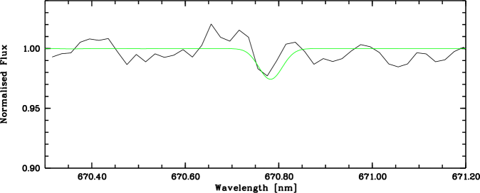
Figure 2: The range of the Li doublet for the star SDSS J082511+163459: the observed spectrum (solid black) is compared to a synthetic profile with A(Li)=1.4 (solid green/grey).

5.3 SDSS J085211+033945

This star, with SDSS J082511+163459, is the most metal-rich of the sample, but being about 900 K hotter than the previous one, its spectrum contains fewer detectable lines, and the abundances of fewer elements can be derived. At variance with SDSS J082511+163459, this star has a clear enhancement in $\alpha$-elements.

We did not use the Ca ii IR triplet, which suffers from the aforementioned sky subtraction problems, affecting in particular the two bluest lines. The $\alpha$ element abundance, [$\alpha$/H]$=-2.86\pm 0.22$ is based on Mg and Ca lines. One single line of Si i indicates that the Si abundance is in agreement with the other $\alpha$ elements. From seven lines of Ti ii, the Ti abundance is found to be about 0.2 dex higher than the stated [$\alpha$/H], with a comparable $\sigma$ of 0.24 dex. The detection of two Al i lines permits us to derive the Al abundance. The two lines of Sr ii are also visible. The abundances of the elements that can be derived from the observed spectra are in Table 6. There is an emission feature at the place of the Li 670.8 nm doublet.

Table 6: SDSS J085211+033945 abundances.

Element	[X/H]fit	N
	x=2.0$\mathrm{km\,s^{-1}}$
Fe i	$-3.24\pm 0.24$	32
Fe ii	$-2.91\pm 0.15$	2
Mg i	$-2.92\pm 0.21$	6
Al i	$-3.77\pm 0.06$	2
Si i	$-3.08$	1
Ca i	$-2.85\pm 0.20$	2
Ca ii	$-2.53$	1
Ti ii	$-2.63\pm 0.24$	7
Sr ii	$-3.04\pm 0.01$	2

5.4 SDSS J090733+024608

There are two Fe ii lines, which provide an iron abundance higher by 0.27 dex than the one derived from the 37 Fe i lines.

Among the six features of Mg detected in the observed spectrum, we retain only four. The bluest line of the Mg i-b triplet, blended with an iron line, very often implies higher abundances than the other two lines of the triplet. We also reject the line at 383.2 nm, which is located on the wing of an H line. For the calcium abundance, we rely on the Ca i lines at 422.6 nm and on the Ca ii-K line. The IR triplet is also detectable, and for this star the sky subtraction is not a problem, but the Ca abundance is much higher ([Ca/H]$=-2.40\pm 0.08$). In this case, we may also suspect deviations from LTE to be the source of the discrepancy. For the [$\alpha$/H]$=-3.11\pm 0.13$ determination, we selected the Mg lines and the Ca lines used for the abundance determination. The Ti abundance, based on five Ti ii lines, is about 0.3 dex higher than the [$\alpha$/H] value. The Cr, Sr, and Ni abundances are each based on one single weak line. Both Sr and Ba are measurable. While Sr is comparable to Fe such that [Sr/Fe]=+0.06, Ba is enhanced by 0.3 dex with respect to iron. The ratio $\left[{\rm Sr/Ba}\right]=-0.36$ corresponds to a pure r-process ratio (see e.g. Qian & Wasserburg 2008). A decrease in temperature does not change this ratio, while a change of $\Delta\xi=\pm 0.5$$\mathrm{km\,s^{-1}}$ results in a change $\Delta\left[{\rm Sr/Ba}\right]=^{-0.42}_{-0.26}$. In any case, the Ba abundance is higher than expected. The individual abundances are listed in Table 7. The Li feature at 670.7 nm is clearly visible, and has an EW of 4 pm meaning an abundance compatible with the Spite plateau, ${\rm A(Li)_{\rm 3D-NLTE}}=2.2$ (see Fig. 3).

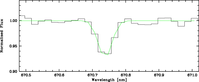
Figure 3: The range of the Li doublet for the star SDSS J090733+024608: the observed spectrum (solid black) is compared to a synthetic profile (solid green/grey). The Li abundance derived is ${\rm A(Li)_{\rm 3D-NLTE}}=2.2$.

Table 7: SDSS J090733+024608 abundances.

Element	[X/H]fit	N
	x=1.8$\mathrm{km\,s^{-1}}$
Fe i	$-3.52\pm 0.16$	37
Fe ii	$-3.25\pm 0.14$	2
Mg i	$-3.14\pm 0.14$	4
Al i	$-4.09\pm 0.06$	2
Ca i	$-3.12$	1
Ca ii	$-2.98$	1
Ti ii	$-2.81\pm 0.09$	5
Sc ii	$-3.14$	1
Cr i	$-3.79$	1
Ni i	$-3.31$	1
Sr ii	$-3.58\pm 0.04$	2
Ba ii	$-3.22$	1

5.5 SDSS J133718+074536

Very few lines are detectable in the spectrum of this “hot” EMP star for a combination of “high” temperature, low metallicity, and low S/N. For these same reasons, the analysis based on the SDSS spectrum relies basically on the K-Ca ii line at 393.3 nm. The continuum determination in this range of the SDSS spectrum is subjective and not trivial, and the calcium line itself has a strange shape, which, at the SDSS spectral resolution and S/N, is compatible with both an extremely low Ca abundance or a damaged line. These findings can explain the large disagreement (–0.91 dex) in the abundances derived from the analyses of the SDSS and X-Shooter spectra.

The X-Shooter observation has a relatively short exposure time because of a change in weather conditions, thus its S/N is lower than desired. Only nine Fe i lines, six Mg i lines, and five Ca lines were detected.

As for the other stars, we do not consider the bluest line of the Mg i-b triplet, because its abundance is too high with respect to the one from the other Mg i lines. In addition the line at 382.9 nm is not included in the abundance determination, leading to a far too high abundance. It was also impossible to reproduce satisfactorily the line profile by synthesis, owing to its placement between two H lines. The Ca i line at 422.6 nm gives an abundance ([Ca/H]=–3.40) in reasonable agreement with the one from the Ca ii-K line, [Ca/H]=–3.23. The abundance of Ca derived from the IR triplet is much higher, $-2.87\pm 0.29$, but the region is badly affected by the sky subtraction. For the $\alpha$ enhancement determination, we take into account the Mg lines included in the sample for the abundance determination, the 422.6 nm Ca i line, and the Ca ii-K line, giving [$\alpha$/H]=$-3.27\pm 0.14$. The individual abundances can be found in Table 8. No spectral line in the wavelength range of the Li doublet at 670.7 nm is clearly visible.

Table 8: SDSS J133718+074536 abundances.

Element	[X/H]fit	N
	x=2.0$\mathrm{km\,s^{-1}}$
Fe i	$-3.49\pm 0.32$	9
Mg i	$-3.24\pm 0.19$	4
Ca i	$-3.40$	1
Ca ii	$-2.96\pm 0.30$	4

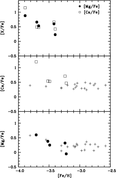
Figure 4: In the upper panel, the abundance of Mg (filled hexagons) and Ca (square) versus [Fe/H]. To derive [Ca/Fe], the lines of Ca ii have been taken into account. The 3D corrections are applied. In middle and lower panel, the 1D-LTE abundances ration [Ca/Fe] and [Mg/Fe], respectively, with the same symbols, are compared to the “First Stars” results (Bonifacio et al. 2009).

6 Kinematics and distance

All the stars have a measured radial velocity above $\simeq 200$km/s except for SDSS J082511+163459, which has a radial velocity of only 24 km/s. This indicates that at least the four high velocity stars could be members of the Galactic halo. We have verified the compatibility of the radial velocity measured with what is expected from the Besançon kinematic model of the Galaxy (Robin et al. 2003). For each star, we simulated a Besançon field of 20 sq deg in the SDSS bands centred on the Galactic coordinates of the given star and then extracted a sample of simulated stars with magnitudes and colors similar to those of the target star. In this way, we checked the radial velocity compatibility with the expected distribution. Owing to the emerging evidence of a Galactic halo populated with substructures (Belokurov et al. 2006), we also explored the possible connection of the stars with some of them, looking for correspondences in distance and in projection on the sky.

We also estimated the distance of each target star by fitting five or eight bands photometry (as given in table 1) with Chieffi et al. (2003) metal-poor isochrones, after correcting for interstellar absorption. The age of the isochrone was fixed at 12.5 Gyr for all the stars and the best-fit model was chosen using a $\chi^{2}$ technique. This is a first rough estimate, which will be refined when a more appropriate set of isochrones (at a compatible low metallicity) become available.

6.1 SDSS J044638-065528

This star has a radial velocity of 242 $\mathrm{km\,s^{-1}}$. With the Besançon model, we have been unable to recover any radial velocity that is so high. We extracted 40 stars within 0.05 mag in terms of color and 0.1 mag in g magnitude around the star. The calculated average ${\rm V_{\rm rad}}$ is 43.2$\mathrm{km\,s^{-1}}$ with a dispersion of $\simeq 50.1$$\mathrm{km\,s^{-1}}$. This object is indeed at about four times the velocity dispersion of the stars in this magnitude range but still at about 2.5 times the velocity dispersion of the Galactic halo. The estimated distance modulus is (m-M)₀=12.90, which corresponds to a distance of 3800 pc. The object does not fall within any known Galactic halo substructure. Moreover, the relatively short distance makes this object an unlikely member of any stream or overdensity.

6.2 SDSS J082511+163459

This object appears to be somewhat more evolved than the remainder of the sample owing to its redder colors. The distance estimate of this star gives a value of 10.9 kpc or a distance modulus of (m-M)₀=15.19. This value places the object above the edge of the Galactic disc in the Monoceros Ring region. A velocity of only 24$\mathrm{km\,s^{-1}}$ implies that this object is a possible member of this structure.

6.3 SDSS J085211+033945

We found that 2% of the objects close to this star in the Besançon simulation have a ${\rm V_{\rm rad}}$ of $\simeq 228\pm 20$$\mathrm{km\,s^{-1}}$. This star is again located on the border of the Monoceros Ring but at half the distance of the previous one, the estimated distance modulus being (m-M)₀=13.75 or 5.6 kpc.

6.4 SDSS J090733+024608

This object and the previous one, SDSS J085211+033945, are close on the sky, within less than six degrees of each other. Distances are also similar, SDSS J090733+024608 being at 4.7 kpc (distance modulus (m-M)₀=13.37). If they also shared the same ${\rm V_{\rm rad}}$, we could try to associate them with a similar feature in the Galactic halo. The measured ${\rm V_{\rm rad}}$ is equal to 304 $\mathrm{km\,s^{-1}}$, which, if the two objects were along a stream, would imply a strong kinematical gradient that has never been observed. If a more precise ${\rm V}_{\rm rad}$ were measured for both objects, we still might be able to associate the two stars.

6.5 SDSS J133718+074536

This star is located toward the the Sagittarius Tidal Arm, which encompass the entire north Galactic cap (Belokurov et al. 2006) at a distance of $\simeq 10.6$ kpc. This is far nearer than the tidal arm, which is located in this region at $\simeq 40$ kpc. A measured ${\rm V}_{\rm rad}$ of 212$\mathrm{km\,s^{-1}}$ implies that this star is most likely to be a member of the Galactic halo.

7 Discussion

7.1 Metallicity distribution function

The results of this observational campaign show that our method for selecting EMP stars from the SDSS spectra is robust. The method relies heavily on the Ca ii K line and has folded-in an assumed $\alpha$ element enhancement [Ca/Fe]$=+0.4$. For stars characterised by a low $\alpha$ to iron ratio, as found in Bonifacio et al. (2011a), the method underestimates the metallicity. The Ca ii K is such a strong line that it is, sometimes, the single detectable feature in a low resolution spectrum of an EMP star. For this reason, several surveys searching for EMP candidates are based on the stellar “metallicity” determination from this line, i.e. the HK survey (Beers et al. 1985, 1992) and the Hamburg-ESO survey (Reimers 1990; Christlieb et al. 2008). In Fig. 5, the measurements of [Fe/H], derived in this work and from UVES spectra in Bonifacio et al. (2011b), is compared to the “metallicity” derived from the SDSS spectra. From the plot, it is clear that down to [Fe/H]$>-3.5$ the agreement is very good, while, at lower metallicities, the metallic lines in the SDSS spectra are very weak, making the low resolution analysis more uncertain. The good agreement between the metallicities estimated from SDSS spectra and the high resolution analysis, shown in Fig. 5, suggests that the metallicities based on the SDSS spectra can be used to trace the low-metallicity tail of the Galactic halo metallicity distribution function. A matter of concern is that below [Fe/H]=–3.5 there is large scatter. In spite of this, we do not conclude that our analysis of the SDSS spectra systematically underestimates the metallicity. By looking at Fig. 5, we see that one star analysed in this paper (SDSS J133718+074536) and another analysed using UVES spectra (Bonifacio et al. 2011b) have a [Fe/H] that is higher by about 1 dex, than the estimate based on the SDSS spectrum. However, a third star (shown with a circle-cross symbol Caffau et al. 2011b), for which we have both X-Shooter and UVES spectra, has a [Fe/H] that is about 1 dex lower. We infer that for [Fe/H]$\lesssim-3.5$ the uncertainty in the metallicity derived from SDSS spectra is about 1 dex, but unbiased.

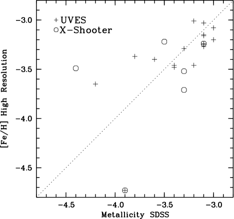
Figure 5: The comparison between the metallicity derived from the low resolution SDSS spectra and our high resolution observations. Crosses represent UVES data (Bonifacio et al. 2011b), and circles the X-Shooter results. The circle-cross symbol is SDSS J102915+172927, discussed in Caffau et al. (2011b), for which we have both X-Shooter and UVES data.

A more robust assessment of the systematics between metallicity estimates derived from SDSS spectra and those based on higher resolution spectra would require the observation of a larger set of stars. The efficiency of X-Shooter suggests that at a rate of 6 stars/night it should be possible to observe about 100 stars in 17 nights. Such an effort, coupled with some higher resolution observations (e.g. with UVES) for the most metal-poor stars, which have hardly any detectable iron lines in the X-Shooter spectra, would allow us to conclusively confirm the almost vertical drop in the metallicity distribution function at [Fe/H]$\sim$–3.5 found for the Hamburg-ESO survey (Reimers 1990; Christlieb et al. 2008) by Schörck et al. (2009). The metallicity distribution function “as observed” for our sample of $\sim$ 125 000 stars does not display this vertical drop (Bonifacio et al. 2010). If the underlying metallicity distribution function is similar to that of Schörck et al. (2009), we expect that the observations with X-Shooter of the 100 most metal-poor stars, according to the SDSS-based estimates, will show that in reality they are of metallicity above [Fe/H]$=-3.5$.

To reconstruct the “true” metallicity distribution function of the Galactic halo it is necessary to correct for the bias present in the SDSS sample. One could argue that there should be no bias, at least in the low metallicity tail, since the $ugriz$ colours become very insensitive to metallicity below [Fe/H]$=-2.0$. Bonifacio et al. (2010) pointed out, by using a photometric metallicity estimate, that the sample of SDSS stars with spectra appeared to have a larger fraction of very metal-poor stars than a random sample, taken from the SDSS database with the same colours. We can obtain an indication of what is boosting the number of metal-poor stars in the sample of stars with SDSS spectra by examining the Object Type keyword of the SDSS spectra of our sample of stars. This keyword contains information on the reason for which the star was selected for SDSS spectroscopy. From Table 2, we see that our targets were observed as either spectrophotometric standards (used for the flux calibration of the spectra), reddening standards, or “serendipity blue”. The sample observed with UVES by Bonifacio et al. (2011b) shows the same descriptors and, in addition a QSO (i.e. the star was expected to be a QSO from its colours). All these classes of objects contain a considerable fraction of very metal-poor stars, thus boosting the numbers in the SDSS spectroscopic database.

7.2 Carbon enhancement

We note that none of the stars observed shows any significant enhancement in carbon. The stars were selected as non-carbon-enhanced from the SDSS spectra. Behara et al. (2010) demonstrated that it is possible to select carbon-enhanced-metal-poor (CEMP) from the SDSS spectra. However, one might have expected that at the higher spectral resolution and S/N of the X-Shooter spectra, some stars classified as non-carbon enhanced based on the SDSS spectra, could display a moderate carbon enhancement. Such star has been found, in contrast to some other studies (Beers et al. 2006).

7.3 $\alpha$ vs. iron abundance

In Fig. 4, we show the ratio of either Mg and Ca to Fe, as a function of iron abundance. The same 3D corrections, derived for the SDSS J044638-065528 star from the 6270 K/4.0/-3.0 model, are applied to all stars. Three stars (SDSS J044638-065528, SDSS J085211+163459, and SDSS J133718+074536) have parameters compatible with the 3D computations. SDSS J090733+024608 is cooler, hence the 3D corrections should be smaller because of the temperature structure of the 3D model, but the microturbulence is 0.5$\mathrm{km\,s^{-1}}$ smaller increasing the 3D corrections. The two effects, at the precision of the present work, cancel out.

The general picture is compatible with what is observed for the sample of EMP stars of Bonifacio et al. (2009) (see middle and lower panels). Star SDSS J044638-065528 displays a rather high $\alpha$ to iron ratio, which appears to be driven by the high Ca abundance. In the lower panel of Fig. 4, we show that 3D corrections are not negligible and provide a closer consistency between the Ca and Mg abundances. The analysis was performed in LTE, although we know that there are indeed NLTE effects on both Mg (Andrievsky et al. 2010) and Ca (Mashonkina et al. 2007). We defer the NLTE analysis to a future paper, but expect this will achieve even closer consistency between Ca and Mg and probably a smaller scatter in the [X/Fe] ratios between different stars, without changing the general pattern.

7.4 Sr and Ba abundances

We find a low [Sr/Ba] ratio of –0.36 for SDSS J090733+024608, which is rather uncommon for metal-poor stars. In the sample of unevolved EMP stars of Bonifacio et al. (2009), none shows such a low Sr/Ba ratio. However, in the sample of giants of François et al. (2007), BD –18^∘ 5550 ([Fe/H]=–3.06) has [Sr/Ba]=–0.27 (see also Andrievsky et al. 2011).

8 Conclusions

We have confirmed the good performance of the X-Shooter IFU (Guinouard et al. 2006), which has been used as an image-slicer, to obtain medium-resolution spectra suitable for abundance analysis. This coupled with the high throughput of X-Shooter has allowed us to investigate several EMP candidate stars in a relatively short time.

The sample of faint distant stars that we have selected as candidate EMP from the SDSS survey has been confirmed to be of extremely low metallicity. Our selection method based on SDSS spectra has been proven to be highly reliable. The chemical composition of our sample appears to be compatible with that found for the much brighter sample of Bonifacio et al. (2009). This may suggest that the stars in the Galactic halo are well mixed throughout its extension. We did not find any $\alpha$-poor stars similar to those found by Bonifacio et al. (2011a). The observations suggest a variability of Li abundances, as already noted in Sbordone et al. (2010) and an absence of a general carbon enhancement among EMP stars.

The observation of a large sample of these candidates extracted from the SDSS is feasible in fewer than 20 nights of observations and would allow us to understand the shape of the metal-weak tail of the Galactic halo metallicity distribution function.