Rescaling multipartite entanglement measures for mixed states

Abstract

A relevant problem regarding entanglement measures is the following: Given an arbitrary mixed state, how does a measure for multipartite entanglement change if general local operations are applied to the state? This question is nontrivial as the normalization of the states has to be taken into account. Here we answer it for pure-state entanglement measures which are invariant under determinant-one local operations and homogeneous in the state coefficients, and their convex-roof extension which quantifies mixed-state entanglement. Our analysis allows us to enlarge the set of mixed states for which these important measures can be calculated exactly. In particular, our results hint at a distinguished role of entanglement measures which have homogeneous degree 2 in the state coefficients.

I Introduction

In recent years, there has been astounding experimental progress in preparing and operating multiqubit entanglement, e.g., with trapped ions Blatt14ions2011 ; FSK2005 , photons Pan2007 ; Weinfurter2009 , and superconducting circuits Martinis2010 ; Schoelkopf2010 . On the other hand, entanglement theory is lagging behind this advancement. To date, it is not possible to adequately characterize the entanglement of an experimentally prepared multipartite quantum state, that is, to quantify how much of a certain type of entanglement is contained in that state.

One difficulty here is that it is not enough to just decide “how much entanglement is present”. Entanglement is regarded as a resource for quantum information tasks, and different tasks require different resources, that is, inequivalent types of entanglement. The criterion whether or not two states can be considered equivalent with respect to their entanglement is whether they can be transformed into one another by means of stochastic local operations and classical communication (SLOCC) Bennett2000 ; DVC2000 . The consequence is that different equivalence classes of entanglement need to be distinguished DVC2000 ; Verstraete2002 ; Lamata2006 ; Bastin2009 .

Entanglement witnesses provide a tool to distinguish SLOCC classes of multipartite states and to experimentally detect them GuehneToth2009 . There are attempts to make witnesses more quantitative Reimpell2007 ; Eisert2007 which have not found widespread application in practice yet.

So far there are only few practically relevant tools for measuring the entanglement of general (mixed) quantum states. Negativity-related entanglement monotones Vidal2002 ; Plenio2005 represent one of them. They are applied only to bipartite systems and it is not clear if they can be used to distinguish different types of entanglement. Therefore we do not further investigate them here. The second well-established tool is Wootters’ approach to compute mixed state entanglement for two qubits Wootters1998 . It is based on the concurrence, a pure-state entanglement measure which is generalizable to pure states of systems larger than two qubits. The kind of pure-state entanglement measures the concurrence belongs to has several interesting properties (see below). In particular, entanglement measures of this kind can distinguish and quantify specific types of multipartite entanglement. Recently there has been progress regarding the question how to obtain SLOCC classifications using them Shelly2010 ; Viehmann2011 ; LiLi2011 . An application of these quantities to mixed states in analogy to Wootters’ method is therefore highly desirable.

The concurrence is an example of a polynomial invariant, i.e., a polynomial function of the coefficients (and not their complex conjugates) of a quantum state, where the function is invariant under determinant-one local operations, that is, under the transformations

$$A = A_{1}\otimes\ldots\otimes A_{N}$$ (1)

$$\equiv \dfrac{F_{1}}{(\det F_{1})^{{1}/{d_{1}}}}\otimes\cdots\otimes\dfrac{F_{N}}{(\det F_{N})^{{1}/{d_{N}}}}\ \ .$$

Here the operators $F_{k}\in\mathrm{GL}(d_{k},\mathbb{C})^{\otimes N}$ represent general (invertible) local operations on the $N$-qudit Hilbert space $\mathcal{H}=\bigotimes_{k=1}^{N}\mathbb{C}^{d_{k}}$. Obviously, $A_{k}$ have determinants equal to 1, i.e., $A_{k}\in\mathrm{SL}(d_{k},\mathbb{C})$.

The peculiarity of polynomial invariants is that a power of them which has homogeneous degree 2 in the state coefficients is automatically an entanglement monotone Verstraete2003 . The generalizations of the concurrence, that is, polynomial invariants for pure states of three and more qubits are well known CKW2000 ; Wong2001 ; LuqueThibon2003 ; OS2005 ; Dokovic2009 .

Hence, pure-state entanglement measures are known in principle at least for multiqubit systems. It is straightforward to generalize them to mixed states via the convex-roof extension Uhlmann1998 (for details, see below). The problem of quantitative entanglement theory is that it is not known how to compute the convex roof of an invariant in general (or even a nontrivial lower bound of it) for any multipartite system, except for the concurrence of two qubits and its straightforward generalization to an even number of qubits, the N-concurrence Uhlmann2000 ; Bullock2004 .

At least there exist a few exact solutions for three-qubit states of low rank and high symmetry Lohmayer2006 ; Eltschka2008 ; Jung2009 ; Fei2011 . To study how to extend these solutions to a larger family of states is part of the quest for a better understanding of the convex roof and multipartite entanglement in mixed states. An important question in this context is how an entanglement measure behaves under general local operations. While local unitary operations represent mere basis changes and do not change entanglement, general local operations require subsequent normalization of the state and thus a conversion of the amount of entanglement.

In this work we investigate how multipartite entanglement needs to be rescaled if it is quantified by functions which are homogeneous and invariant under determinant-one SLOCC operations. It will turn out that in the case of mixed states this is easily done only for the convex roof of pure-state measures with homogeneous degree 2. That is, from the point of view of mixed-state entanglement rescaling, one can conclude that there is a preferred homogeneity degree of pure-state entanglement measures.

The outline of this article is as follows. First we analyze the rescaling properties of the convex-roof extension. Then we illustrate their application (and also their failure for the “wrong” homogeneity degree) by reconsidering some of the known exact solutions. Finally, we mention also some ways to extend the number of exactly solvable three-qubit problems.

II The rescaling method

This section provides the theoretical concepts on which this article is based. They are formulated for general homogeneous invariants, but we interpret them with regard to the physically relevant polynomial $\mathrm{SL}(d_{k},\mathbb{C})^{\otimes N}$-invariants. To begin with, we introduce our notation and explain how a homogeneous invariant of pure states needs to be rescaled under a symmetry transformation if one exclusively focuses on normalized states. Then we explain the convex-roof extension. Finally, we state, derive, and discuss our main results. They describe the scaling of the convex-roof extension of a homogeneous invariant under a symmetry transformation for normalized mixed states.

II.1 Rescaling of homogeneous invariants for normalized pure states

We consider a real function $\tau$ on some finite-dimensional Hilbert space $\mathcal{H}$ that is invariant with respect to some invertible linear operator $L$ acting on $\mathcal{H}$. In formulas, $\tau(L\psi)=\tau(\psi)$ for all $\psi\in\mathcal{H}$. This implies $\tau(L^{-1}\psi)=\tau(\psi)$. We assume further that $\tau$ is homogeneous of degree $\eta$. That is, for positive $\alpha$, $\tau(\alpha\psi)=\alpha^{\eta}\tau(\psi)$. If we focus on normalized states $\phi$ and $\phi^{\prime}$ which are related by $L$ according to $\phi^{\prime}=L\phi/||L\phi||$, it follows that

$$\tau(\phi^{\prime})=\dfrac{\tau(\phi)}{||L\phi||^{\eta}}.$$ (2)

Note that $\tau$ could be one of the polynomial invariants discussed in the introduction (or a function thereof) if $\mathcal{H}=\bigotimes_{k=1}^{N}\mathbb{C}^{d_{k}}$ and $L\equiv A\in\mathrm{SL}(d_{k},\mathbb{C})^{\otimes N}$. Note further that Eq. (2) has the same form for all $\eta$, so that there is no preferred homogeneity degree for the polynomial invariant.

II.2 The convex roof extension

Let $\mathcal{H}$ be a finite-dimensional Hilbert space and $\Omega_{\mathcal{H}}$ the convex set of (normalized) density operators acting on $\mathcal{H}$. All $\rho\in\Omega_{\mathcal{H}}$ can be written as convex sums $\rho=\sum_{i}p_{i}\pi_{i}$. That is, $p_{i}\geq 0$, $\sum_{i}p_{i}=1$, and $\pi_{i}$ is an extreme point of $\Omega_{\mathcal{H}}$. An extreme point $\pi$ of $\Omega_{\mathcal{H}}$ is given by $\pi=\left|\psi\right>\!\left<\psi\right|/||\psi||^{2}$, where $\psi\in\mathcal{H}$ ($\neq 0$), and is usually referred to as a pure state. A mixed state $\rho$ has rank $>1$, and its decomposition $\{p_{i},\pi_{i}\}$ into pure states is not unique Schroedinger1936 .

A real continuous function $f$ on $\mathcal{H}$ can be extended to $\Omega_{\mathcal{H}}$ via convex-roof extension Uhlmann1998 :

$$f(\rho)=\mathrm{min}\sum_{i}p_{i}f(\pi_{i}).$$ (3)

The minimum runs over all possible decompositions of $\rho$ into pure states, and $f(\pi_{i})\equiv f(\psi_{i}/||\psi_{i}||)$. A decomposition $\{\tilde{p}_{i},\tilde{\pi}_{i}\}$ of $\rho$ for which $f(\rho)=\sum\tilde{p}_{i}f(\tilde{\pi}_{i})$ is called optimal. The minimal length of an optimal decomposition (the minimal number of pure states in the decomposition) is $\leq(\mathrm{rank}\rho)^{2}$ (this is a consequence of Carathéodory’s theorem, see Ref. Uhlmann1998 , Lemma 1). Since $f(\rho)$ is an entanglement monotone on $\Omega_{\mathcal{H}}$ if $f$ is an entanglement monotone on $\mathcal{H}$ Vedraletal1997 ; Vidal2000 , the convex-roof extension is the standard way of applying a pure-state entanglement measure to mixed states. For further properties of the convex-roof extension, see Uhlmann1998 ; Uhlmann2000 ; Vidal2000 . However, as mentioned, finding the minimum in Eq. (3) is difficult in general.

II.3 The convex-roof extension of homogeneous invariants

Let us now investigate how the convex-roof extension of $\tau$ transforms under the action of $A$, that is, how $\tau(\rho)$ and $\tau(\rho^{\prime})$ are related if $\rho^{\prime}=L\rho L^{\dagger}/\mathrm{tr}L\rho L^{\dagger}$ $(\rho,\rho^{\prime}\in\Omega_{\mathcal{H}})$. Interestingly, it turns out that the convex-roof extension does not lead to a simple generalization of Eq. (2) for all $\eta$. Rather, the convex-roof extension singles out invariants of homogeneous degree $\eta=2$. Only in that case the convex-roof extension of $\tau$ generally can be rescaled as for pure states,

$$\tau(\rho^{\prime})=\dfrac{\tau(\rho)}{\mathrm{tr}L\rho L^{\dagger}}\ \ .$$ (4)

This formula represents the case $\eta=2$ of a naive generalization of Eq. (2) to $\tau(\rho^{\prime})\stackrel{{\scriptstyle?}}{{=}}\tau(\rho)/(\mathrm{tr}L\rho L^{\dagger})^{\eta/2}$ which, however, is not correct in general. The main conclusions of this article are based on formula (4). We will see that it can be understood as a consequence of the fact that $L$ maps an optimal decomposition of $\rho$ onto an optimal decomposition of $\rho^{\prime}$ if $\eta=2$. For $\eta\neq 2$, the invariance of $\tau$ under $L$ still guarantees that $\tau(\rho)$ and $\tau(\rho^{\prime})$ are either both zero or both nonzero if $\tau(\psi)\geq 0$. These results give information about the convex roof of $\tau$ for $\rho^{\prime}$ if it is known for $\rho$. Applying them to the polynomial invariants allows us to extend (previous) results for the entanglement of a mixed state as measured by the polynomial invariants to all states that can be obtained from this state via general invertible local operations $F$ (ILOs): If $F=F_{1}\otimes\ldots\otimes F_{N}\in\mathrm{GL}(d_{k},\mathbb{C})^{\otimes N}$, then

$$\rho^{\prime} =\dfrac{F\rho F^{\dagger}}{\mathrm{tr}F\rho F^{\dagger}}=\dfrac{A\rho A^{\dagger}}{\mathrm{tr}A\rho A^{\dagger}},$$ (5)

where $A\in\mathrm{SL}(d_{k},\mathbb{C})^{\otimes N}$ is defined as in Eq. (1). An example that illustrates how Eq. (4) can be utilized to calculate the three-tangle of mixed states will be presented in the next section.

In order to see how Eq. (4) is obtained, suppose that $\{p_{i},\pi_{i}\}$ and $\{q_{j},\varpi_{j}\}$ are optimal decompositions of $\rho$ and $\rho^{\prime}$ of lengths $m$ and $n$, respectively. In other words, $\tau(\rho)=\sum_{i=1}^{m}p_{i}\tau(\pi_{i})$ and $\tau(\rho^{\prime})=\sum_{j=1}^{n}q_{j}\tau(\varpi_{j})$. We express $\rho^{\prime}$ in terms of the $\{p_{i},\pi_{i}\}$ and $\rho$ in terms of the $\{q_{j},\varpi_{j}\}$,

$$\rho =\sum_{i=1}^{m}{p_{i}\pi_{i}}=\sum_{j=1}^{n}{q_{j}^{\prime}\varpi_{j}^{\prime}},$$ (6)

$$\rho^{\prime} =\sum_{j=1}^{n}{q_{j}\varpi_{j}}=\sum_{i=1}^{m}{p_{i}^{\prime}\pi_{i}^{\prime}},$$ (7)

where

$$p_{i}^{\prime} =p_{i}T^{-1}\mathrm{tr}L\pi_{i}L^{\dagger},\; q_{j}^{\prime} =q_{j}T\mathrm{tr}[L^{-1}\varpi_{j}(L^{-1})^{\dagger}],$$ (8)

$$\pi_{i}^{\prime} =\dfrac{L\pi_{i}L^{\dagger}}{\mathrm{tr}L\pi_{i}L^{\dagger}},\; \varpi_{j}^{\prime} =\dfrac{L^{-1}\varpi_{j}(L^{-1})^{\dagger}}{\mathrm{tr}[L^{-1}\varpi_{j}(L^{-1})^{\dagger}]}.$$ (9)

We have used the abbreviation $T=\mathrm{tr}L\rho L^{\dagger}$. It is easy to see that $\sum_{i}p_{i}^{\prime}=\sum_{j}q_{j}^{\prime}=1$ and that $\pi_{i}^{\prime}$ and $\varpi_{j}^{\prime}$ are pure states. Since $L\pi_{i}L^{\dagger}(=L\pi_{i}\pi_{i}^{\dagger}L^{\dagger})$ is a positive operator and $L$ is invertible, $\mathrm{tr}L\pi_{i}L^{\dagger}>0$. Consequently, $T>0$. A similar argument ensures that $\mathrm{tr}[L^{-1}\varpi_{j}(L^{-1})^{\dagger}]>0$. Starting from Eqs. (6) and (7), one can estimate

$$\tau(\rho) \leq T\sum_{j=1}^{n}q_{j}[\mathrm{tr}L^{-1}\varpi_{j}(L^{-1})^{\dagger}]^{\frac{2-\eta}{2}}\tau(\varpi_{j}),$$ (10)

$$\tau(\rho^{\prime}) \leq T^{-1}\sum_{i=1}^{m}p_{i}[\mathrm{tr}L\pi_{i}L^{\dagger}]^{\frac{2-\eta}{2}}\tau(\pi_{i}).$$ (11)

If $\eta=2$, Eq. (4) follows. Moreover, one sees that $\{p_{i}^{\prime},\pi_{i}^{\prime}\}$ is an optimal decomposition of $\rho^{\prime}$ because $\sum_{i}p_{i}^{\prime}\tau(\pi_{i}^{\prime})=\sum_{i}p_{i}\tau(\pi_{i})/T=\tau(\rho)/T$. Further, $\{q_{j}^{\prime},\varpi_{j}^{\prime}\}$ is an optimal decomposition of $\rho$. Hence, an optimal decomposition $\{p_{i},\pi_{i}\}$ ($\{q_{j},\varpi_{j}\}$) of $\rho$ ($\rho^{\prime}$) is mapped by $L$ ($L^{-1}$) onto an optimal decomposition of $\rho^{\prime}$ ($\rho$) which is given by $\{p_{i}^{\prime},\pi_{i}^{\prime}\}$ ($\{q_{j}^{\prime},\varpi_{j}^{\prime}\}$) in Eqs. (8) and (9).

If $\eta\neq 2$, but $\tau\geq 0$, one can still conclude from Eqs. (10) and (11) that either both $\tau(\rho)$ and $\tau(\rho^{\prime})$ are zero or both are nonzero. The assumption $\tau(\rho)=0$ implies $\tau(\pi_{i})=0$ for all $\pi_{i}$ and, due to Eq. (11), $\tau(\rho^{\prime})=0$. On the other hand, the assumption $\tau(\rho)>0$ implies that $\tau(\varpi_{j})>0$ for at least one $\varpi_{j}$ because of Eq. (10). The converse follows analogously.

Let us briefly discuss these results with regard to the polynomial invariants and their application as entanglement measures. As already indicated, our results, in particular Eq. (4), provide a useful tool for learning about the convex-roof extension of a polynomial invariant for a mixed state $\rho^{\prime}$ if it is already known for a state $\rho$ that can be transformed into $\rho^{\prime}$ via SLOCC. However, we have also gained another important insight about the convex-roof extension of polynomial invariants: It has peculiar properties for polynomial entanglement measures of homogeneity degree 2 (or, of linear degree if the pure-state measures are regarded as functions of rank-one density operators) and therefore indicates a special significance of the latter. Only for entanglement measures of this type, the invariance property for normalized pure-states generalizes to normalized mixed states and the entanglement both of pure and mixed SLOCC-equivalent states is related by a simple analytical formula, Eq. (4).

III Examples

Now we consider several examples to illustrate how the rescaling method from Section II can be applied to generalize existing results for mixed-state entanglement. We will also demonstrate what happens if one tries to apply it to monotones of degree $\neq 2$.

The examples we consider are mixed states of three qubits. For three-qubit systems, there is only one polynomial $\mathrm{SL}(2,\mathbb{C})^{\otimes 3}$ invariant, the three-tangle CKW2000 . For $\left|\psi\right>=\sum_{i,j,k=0}^{1}\psi_{ijk}\left|ijk\right>$ it is given by

$$\tau_{3}(\psi) = 4\left|d_{1}-2d_{2}+4d_{3}\right|,$$

$$d_{1} = \psi_{000}^{2}\psi_{111}^{2}+\psi_{001}^{2}\psi_{110}^{2}+\psi_{010}^{2}\psi_{101}^{2}+\psi_{011}^{2}\psi_{100}^{2}$$

$$d_{2} = \psi_{000}\psi_{001}\psi_{110}\psi_{111}+\psi_{000}\psi_{010}\psi_{101}\psi_{111}+$$

$$+\psi_{000}\psi_{011}\psi_{100}\psi_{111}+\psi_{001}\psi_{010}\psi_{101}\psi_{110}+$$

$$+\psi_{001}\psi_{011}\psi_{100}\psi_{110}+\psi_{010}\psi_{011}\psi_{100}\psi_{101}$$

$$d_{3} = \psi_{000}\psi_{110}\psi_{101}\psi_{011}+\psi_{100}\psi_{010}\psi_{001}\psi_{111}$$ (12)

and distinguishes Greenberger-Horne-Zeilinger (GHZ) entanglement from $W$-type entanglement. For mixed states, it is defined by convex-roof extension.

The three-tangle has homogeneous degree $4$. However to apply the rescaling method Eq. (4) as described above, degree $2$ is required. Therefore on pure states we have to use the square root of the three-tangle, $\tau(\psi)=\sqrt{\tau_{3}(\psi)}$ which is an entanglement monotone as well Duer2000 . For mixed states, we again define $\tau(\rho)$ through the convex-roof extension. Note that this is not the same as taking the square root of $\tau_{3}(\rho)$. However $\tau(\rho)=0$ iff $\tau_{3}(\rho)=0$; therefore both are equally suitable to distinguish GHZ-type and $W$-type entanglement.

III.1 Mixtures of generalized GHZ and $W$ states

We consider $\tau(\rho)$ for rank-2 mixtures

$$\rho(p)=p\left|\mathrm{gGHZ}\right>\!\left<\mathrm{gGHZ}\right|+(1-p)\left|\mathrm{g}W\right>\!\left<\mathrm{g}W\right|$$ (13)

of a generalized GHZ and generalized $W$ state (both normalized)

$$\left|\mathrm{gGHZ}\right>\ = \ a\left|000\right>+b\left|111\right>$$

$$,\left|\mathrm{g}W\right>\ = \ c\left|100\right>+d\left|010\right>+e\left|001\right>\ \ .$$ (14)

The three-tangle of those states has been calculated in Eltschka2008 . We will be able to reuse pure-state results from that paper.

We begin by solving the problem using the characteristic curve method OSU2008 and then demonstrate how those solutions can be mapped to each other by means of the rescaling method.

The characteristic curve is defined as the minimum tangle of the states at the same “height” in the Bloch sphere as the corresponding mixed state,

$$\tilde{\tau}(p)=\min_{\phi}(\tau(\sqrt{p}\left|\mathrm{gGHZ}\right>+\sqrt{1-p}\mathrm{e}^{\mathrm{i}\phi}\left|\mathrm{g}W\right>)).$$ (15)

Since we are dealing with pure states at this point, and the square root is monotonic, we can reuse the results of Ref. Eltschka2008 and get

$$\tilde{\tau}(p)=2\left|ab\right|\sqrt{\left|p^{2}-|s|\sqrt{p(1-p)^{3}}\right|}$$ (16)

where we have used the definition

$$s=\frac{4cdf}{a^{2}b}\ \ .$$ (17)

The convex characteristic curve $\tau_{s}^{*}(p)$ is the function convex hull of $\tilde{\tau}(p)$, i. e., the largest convex function which is nowhere larger than $\tilde{\tau}(p)$. As shown in Ref. OSU2008 , the convex characteristic curve is always a lower limit to $\tau(p)$. Using the results in Eltschka2008 , we find that $\tilde{\tau}(p)$ has zeros at $p=0$ and at $p=p_{0}$ with

$$p_{0}=\frac{|s|^{\frac{2}{3}}}{1+|s|^{\frac{2}{3}}}\ \ .$$ (18)

It is easy to check that for $p>p_{0}$, $\tilde{\tau}(p)$ is concave (note that this is different from the three-tangle itself where $\tilde{\tau}_{3}(p)$ is convex right above $p_{0}$ for $s<2\sqrt{2}$). Therefore, in this region, the convex characteristic curve is a straight line. We thus get

$$\tau^{*}(p)=\begin{cases}0&\mbox{for }0\leq p\leq p_{0},\\ 2\left|ab\right|\left(p-(1-p)|s|^{\frac{2}{3}}\right)&\mbox{for }p_{0}\leq p\leq 1.\end{cases}$$ (19)

In the current case, the convex characteristic curve actually gives the correct value of $\tau(p)$. This can be seen from the symmetry of the problem: Applying the local unitary transformation

$$U_{3}=\exp\left[\frac{\mathrm{i}\pi}{3}\sigma_{z}^{(1)}\right]\exp\left[\frac{\mathrm{i}\pi}{3}\sigma_{z}^{(2)}\right]\exp\left[\frac{\mathrm{i}\pi}{3}\sigma_{z}^{(3)}\right]$$ (20)

changes neither the GHZ nor the $W$ state (and thus also not their mixtures) and, of course, nor the three-tangle. But it changes the relative phase between the GHZ and the $W$ state in the superpositions of Eq. (15), thus rotating the Bloch sphere spanned by these superpositions by $2\pi/3$. Thus each state gives rise under this symmetry $U_{3}$ to three locally SU equivalent states whose equal mixture gives exactly $\rho(p)$ (Eq. (13)). This is especially true for the minimum $\tau$ state defining the characteristic curve. Thus, due to the symmetry the characteristic curve gives an upper limit to $\tau$.

Since the convex characteristic curve always provides a lower limit, wherever both agree, the unconvexified curve gives the correct tangle, and therefore in those points the above decomposition is an optimal one.

While the above argument applies only to the points $p=0$, $p=p_{0}$, and $p=1$, it is obvious that for the linear sections of the convex characteristic curves, the value $\tau^{*}(p)$ can be achieved by appropriately combining the optimal decompositions of the corresponding end points which proves that indeed $\tau(\rho(p))=\tau^{*}(p)$.

After deriving the solution of the problem, we now show that different states (13) are SLOCC equivalent and, hence, that the solutions $\tau$ for different values of $a,\ldots,f$ can be obtained from each other via the rescaling method. To this end, we apply a diagonal invertible local operation of determinant one,

$$A=\left(\begin{matrix}\alpha&0\\ 0&1/\alpha\end{matrix}\right)\otimes\left(\begin{matrix}\beta&0\\ 0&1/\beta\end{matrix}\right)\otimes\left(\begin{matrix}\gamma&0\\ 0&1/\gamma\end{matrix}\right),$$ (21)

which transforms $\left|\mathrm{gGHZ}\right>$ to $\mathcal{N}_{1}\left|\mathrm{GHZ}\right>$ and $\left|\mathrm{g}W\right>$ to $\mathcal{N}_{2}\left|W\right>$. An easy calculation shows that this is achieved for

$$\alpha=\left(\frac{bc^{2}}{adf}\right)^{\frac{1}{6}},\quad\beta=\left(\frac{bd^{2}}{acf}\right)^{\frac{1}{6}},\quad\gamma=\left(\frac{bf^{2}}{acd}\right)^{\frac{1}{6}}.$$ (22)

This transforms $\left|\mathrm{gGHZ}\right>$ into $\sqrt{2ab}\left|\mathrm{GHZ}\right>$ and $\left|\mathrm{g}W\right>$ into $\sqrt{3}\left(\sqrt{\frac{b}{a}}cdf\right)^{\frac{1}{3}}\left|W\right>=\sqrt{\frac{3}{8}}\cdot\sqrt{2ab}\cdot(2s)^{\frac{1}{3}}\left|W\right>$ and therefore $\rho$ into

$$A\rho A^{\dagger}=2\left|ab\right|\left(p\left|\mathrm{GHZ}\right>\!\left<\mathrm{GHZ}\right|+\frac{3(1-p)}{8}\left|2s\right|^{\frac{2}{3}}\left|W\right>\!\left<W\right|\right).$$ (23)

Since the trace of this operator is

$$T\ \equiv\ \operatorname{tr}(A\rho A^{\dagger})=2\left|ab\right|\left(p+\frac{3(1-p)}{8}\left|2s\right|^{2/3}\right),$$ (24)

we have to divide $\rho^{\prime}$ by this expression and find

$$\rho^{\prime}=\frac{A\rho A^{\dagger}}{T}=p^{\prime}\left|\mathrm{GHZ}\right>\!\left<\mathrm{GHZ}\right|+(1-p^{\prime})\left|W\right>\!\left<W\right|$$ (25)

with

$$p^{\prime}\ =\ \frac{p}{p+\frac{3(1-p)}{8}|2s|^{2/3}}$$ (26)

or, solving for $p$,

$$p\ =\ \frac{3p^{\prime}|2s|^{2/3}}{3p^{\prime}|2s|^{2/3}+8(1-p^{\prime})}$$ (27)

Note that this is an increasing function of $p^{\prime}$.

Now we can apply the rescaling method described in the previous section to this problem. By using Eq. (4) we obtain

$$\tau(\rho(p))=T\ \tau(\rho^{\prime}(p^{\prime})),$$ (28)

where $T$ is taken from Eq. (24), and $p^{\prime}$ from (26).

For the standard GHZ/$W$ problem, that is, $a=b$ and $c=d=f$, we have $s=2^{7/2}/3^{3/2}$ and $2|ab|=1$, and therefore,

$$\tau(\rho^{\prime}(p^{\prime}))=\begin{cases}0&\mbox{for }0\leq p^{\prime}\leq p^{\prime}_{0}=\frac{2^{7/3}}{3+2^{7/3}},\\ p^{\prime}-(1-p^{\prime})\frac{2^{7/3}}{3}&\mbox{for }p^{\prime}_{0}\leq p^{\prime}\leq 1.\end{cases}$$ (29)

By inserting all values one indeed recovers Eq. (19) with the correct value of $p_{0}$, Eq. (18), see Fig. 1. This means in turn that, by virtue of the rescaling method, the knowledge of the solution of the standard problem with symmetric GHZ and $W$ states in Eq. (29) is sufficient to obtain the solution of the more general states in Eq. (13). This is achieved simply by applying ILOs according to Eq. (21) and appropriate rescaling following Eq. (4).

Figure 1: Illustration of the rescaling method for the square root of the three-tangle $\tau$ of mixtures of standard (left) and generalized (right) GHZ and $W$ states. The two orthogonal eigenstates (g)GHZ and (g)$W$ are located at the north and south poles of the Bloch spheres, respectively, and the mixing parameters $p^{\prime}$, $p$ vary along the lines connecting the two poles. The symmetric GHZ/$W$ problem (left) can be transformed into the generalized GHZ/$W$ problem (right) and vice versa by an invertible local operation. The corners of the tetrahedra show the pure states of the optimal decomposition of the states inside those tetrahedra. In the lower (blue) tetrahedron, $\tau=0$, while in the upper (green) tetrahedron, it grows linearly with $p^{\prime}$ ($p$). If the convex-roof extension is known for one of the problems, it can be calculated for the other by virtue of the rescaling method.

Note that while we have considered only diagonal transformations, the method is of course valid for general invertible local operations. Those break the symmetry noted above and therefore lead to cases which cannot be solved using the convex characteristic curve method. For those problems, no general method is yet known.

III.2 Using the rescaling method for degrees other than $2$

As mentioned before, the rescaling method is not fully applicable to entanglement measures with homogeneous degree $\eta\neq 2$. However, by considering the three-tangle ($\eta=4$) of GHZ/$W$ mixtures we will see that if the problem has certain symmetries, the rescaling method can still be useful for calculating entanglement measures with $\eta\neq 2$.

The three-tangle of the mixtures in Eq. (13) has already been calculated in Eltschka2008 and, for the special case of mixing standard GHZ and standard $W$, in Lohmayer2006 (see also Fig. 2).

Figure 2: Illustration of the three-tangle $\tau_{3}$ of mixtures of standard GHZ and $W$ states and generalized GHZ and $W$ states. As in Fig. 1, the (g)GHZ and (g)$W$ states are at the north and south poles of the Bloch spheres, respectively, and the corners of the tetrahedra and triangles give the elements of the optimal decompositions. In each red triangle, $\tau_{3}=\mathrm{const}$. In the blue tetrahedra, $\tau_{3}=0$, and in the green tetrahedra $\tau_{3}$ depends linearly on the mixing parameter. Here, the sphere in the center represents the standard GHZ/$W$ case. The transformation to the generalized problem leads to two different cases: For $s<2\sqrt{2}$ (left sphere), the structure of the symmetric case is preserved. However, for $s>2\sqrt{2}$, the two tetrahedra sit directly on top of each other. As states equivalent under ILOs can have optimal decompositions for $\tau_{3}$ with different lengths, the figure indicates that the rescaling method cannot be applied to calculate $\tau_{3}$.

For the mixtures of standard GHZ and standard $W$, the three-tangle has the form

$$\tau_{3}(p^{\prime})=\begin{cases}0,&0\leq p^{\prime}\leq p^{\prime}_{0},\\ p^{\prime 2}-\frac{2^{7/2}}{3^{3/2}}\sqrt{p^{\prime}(1-p^{\prime})^{3}},&p^{\prime}_{0}\leq p^{\prime}\leq p^{\prime}_{1},\\ 1-(1-p^{\prime})\left(\frac{3}{2}+\frac{1}{18}\sqrt{465}\right),&p^{\prime}_{1}\leq p^{\prime}\leq 1,\end{cases}$$ (30)

where $p^{\prime}_{0}=\frac{2^{7/3}}{3+2^{7/3}}$ and $p^{\prime}_{1}=\frac{1}{2}+\frac{1}{18}\sqrt{465}$. We now derive the results of a simple-minded application of the rescaling method to the three-tangle which is based on the naive generalization of Eq. (2) (below Eq. (4)) with $\eta=4$. That is, we calculate $p^{\prime}$ from $p$ using Eq. (26), apply the function above, and then multiply with $T^{2}$ from Eq. (24). It will turn out that this procedure indeed leads to incorrect results in general.This is also suggested by Fig. 2: Optimal decompositions of states which can be transformed into one another by means of operations Eq. (21) can have different lengths. Hence, the ILOs in general do not map optimal decompositions onto optimal decompositions, and one would therefore not expect that the three-tangle of a mixed state can be traced back to the (known) three-tangle of an SLOCC-equivalent state via the rescaling method. However, we will also see that in some cases the correct three-tangle of mixtures of generalized GHZ and $W$ states can be obtained from Eqs. (30) by means of this method due to the particular symmetries of this problem.

To identify the range of $p$ where the three-tangle vanishes, we insert $p^{\prime}_{0}$ into Eq. (27) and get Eq. (18) in agreement with Ref. Eltschka2008 . Indeed this was to be expected, because the method allows us to reliably distinguish between zero and nonzero values of the polynomial even for homogeneity degrees other than 2.

Next, we calculate the tangle for $p_{0}\leq p\leq p_{1}$ using the method above, where $p_{1}$ is the $p$ value beyond that $\tau_{3}(\rho(p))$ increases linearly Eltschka2008 . From

$$\tau_{3}(\rho(p))=T^{2}\tau_{3}(\rho^{\prime}(p^{\prime}))$$ (31)

we get

$$\tau_{3}(p)=4\left|ab\right|^{2}\left(p^{2}-|s|\sqrt{p(1-p)^{3}}\right)$$ (32)

which again agrees exactly with the result in Ref. Eltschka2008 . This comes somewhat as a surprise, because the method should not be applicable here. However, it is easily explained by considering the symmetry of the problem.

Let us consider the special case that both $\{p_{i},\pi_{i}\}$ and $\{p_{i},A\pi_{i}A^{\dagger}/T\}$ are optimal decompositions of $\rho$ and $\rho^{\prime}$ in normalized pure states. This implies $\mathrm{tr}(A\pi_{i}A^{\dagger})=T$ for all $i$. One easily sees from Eqs. (10) and (11) that, under these conditions, $\tau(\rho)=T^{\eta/2}\tau(\rho^{\prime})$ if $\tau$ is an arbitrary homogeneous invariant, or, in the case of the three-tangle, $\tau_{3}(\rho)=T^{2}\tau_{3}(\rho^{\prime})$. The specific mixed states and ILOs of our example satisfy these conditions for $p_{0}\leq p\leq p_{1}$, as we now explain.

In this region characteristic curve and convex characteristic curve agree with each other. As described above, this is because there is an optimal decomposition which consists purely of states related by the local symmetry (20) which rotates the Bloch sphere by $2\pi/3$.

Arbitrary rotations of the Bloch sphere about the GHZ/$W$ axis cannot be achieved by local operations; however, they can be realized by nonlocal diagonal unitary transformations, e.g., $U(\varphi)=\operatorname{diag}(1,\mathrm{e}^{\mathrm{i}\varphi},\mathrm{e}^{\mathrm{i}\varphi},\mathrm{e}^{-\mathrm{i}\varphi},$ $\mathrm{e}^{\mathrm{i}\varphi},\mathrm{e}^{-\mathrm{i}\varphi},\mathrm{e}^{-\mathrm{i}\varphi},1)$. Note that the local operations (20) are a subset of these. Now the ILOs (21) are also diagonal and therefore commute with those transformations. This means especially that if two vectors are equivalent under this symmetry $U(\varphi)$, the transformed vectors are also equivalent under this symmetry, which means that horizontal planes in the Bloch sphere are just moved vertically by the transformation. Moreover, it is easy to verify that if two pure states can be transformed into each other by $U(\varphi)$, i.e., share the same latitude, their norms are also multiplied by the same factor. This implies that for those states, the transformed state has minimal three-tangle iff the original state had minimal three-tangle. Of course, all convex combinations of those states are also multiplied with the same factor. Especially, the characteristic curve of the original problem is mapped onto the characteristic curve of the transformed problem.

However, to get the correct three-tangle, one needs the convex characteristic curve, which does not agree with the characteristic curve above $p_{1}$. Now we cannot expect that the transform of the latter gives the same result as the convexification of the transformed curve and that optimal decompositions are mapped to optimal decompositions in general. Indeed, trying a straightforward calculation of $p_{1}$ using Eq. (27), we obtain

$$p_{1}^{\text{Eq. (\ref{eq:pfromptilde})}}=\frac{24\ |2s|^{\frac{2}{3}}}{91-3\sqrt{465}+24\ |2s|^{\frac{2}{3}}}$$ (33)

which not only does not agree with the correct $p_{1}$ from Eltschka2008 , but even has a wrong behavior. While the correct $p_{1}$ decreases from $1$ to $1/2$ on increasing $s$ (actually, only until it hits $p_{0}$), $p_{1}^{\text{Eq. (\ref{eq:pfromptilde})}}$ instead increases from $0$ to $1$.

As the unconvexified characteristic curve is mapped onto the unconvexified characteristic curve of the transformed problem, the correct three-tangle can be obtained by using the former to calculate the convex characteristic curve directly. However, we emphasize again that this is only due to the high symmetry of the problem and the fact that the symmetry operations commute with the diagonal ILOs.

As in the case of degree 2 (Section III.1), one might consider to further extend the range of solutions derived from the standard GHZ/$W$ case by applying arbitrary (i.e., not only diagonal ones) local SL transformations. However, general transformations modify the unitary symmetry of the problem into one which is nonunitary, $AU(\varphi)A^{-1}$. Such a transformation in general does not map the characteristic curve (and the optimal decompositions) of the standard GHZ/$W$ mixtures onto the characteristic curve (and the optimal decompositions) of the transformed mixed states. Therefore, in general the rescaling method is not useful for finding new solutions for the convex roofs of entanglement measures with homogeneity degree $\eta\neq 2$. However, note that the zero polytope of the original problem will be mapped exactly onto the zero polytope of the transformed problem, irrespective of $\eta$ (see Section II).

III.3 Using the rescaling method for mixed states of rank greater than $2$

If the degree of homogeneity of the polynomial invariant is 2, the rescaling method is fully applicable. We show now by discussing further examples that it can be also successfully employed for calculating the entanglement of mixed states with rank $>2$. Consider, for instance, rank-3 mixtures of $\left|\mathrm{GHZ}\right>$, $\left|W\right>$ and $\left|\bar{W}\right>=(\left|011\right>+\left|101\right>+\left|110\right>)/\sqrt{3}$. The three-tangle for such mixtures has been found by Jung et al. Jung2009 . We illustrate the application of the rescaling method for states of rank $>2$ by briefly sketching how the square root of the three-tangle can be obtained for those states and all SLOCC equivalent states. Adopting the parameterization from Ref. Jung2009 , we have

$$\rho(p,q)=p\left|\mathrm{GHZ}\right>\!\left<\mathrm{GHZ}\right|+q\left|W\right>\!\left<W\right|+(1-p-q)\left|\bar{W}\right>\!\left<\bar{W}\right|.$$ (34)

The analog of the characteristic curve is now the two-dimensional “characteristic surface”

$$\tilde{\tau}(p,q)\ = \ \min_{\phi_{1},\phi_{2}}\tau\left[\sqrt{p}\left|\mathrm{GHZ}\right>-\right.$$ (35)

$$\left.-\sqrt{q}\mathrm{e}^{\mathrm{i}\phi_{1}}\left|W\right>-\sqrt{1-p-q}\mathrm{e}^{\mathrm{i}\phi_{2}}\left|\bar{W}\right>\right],$$

where $\tau=\sqrt{\tau_{3}}$. We have again adopted the parameterization of the states used in Jung2009 . As before, the problem has the symmetry (20), and an equal mixture of a set of states equivalent to a given state under this symmetry states gives $\rho(p,q)$. It is easy to see that $\tau$ takes its minimal value for $\phi_{1}=\phi_{2}=0$, which results in

$$\tilde{\tau}(p,q)=\sqrt{\left|p^{2}-4p\sqrt{qr}-\frac{4}{3}qr-\frac{8\sqrt{6}}{9}\left(\sqrt{pq^{3}}+\sqrt{pr^{3}}\right)\right|},$$ (36)

where we have defined $r=1-p-q$. The decompositions of $\rho(p,q)$ leading to those values (note that in general they do not represent the optimal decompositions because the surface is not convex) are the ones given in Eq. (11) of Jung2009 .

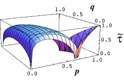
Figure 3: Characteristic surface $\tilde{\tau}(p,q)$ (Eq. (36)) for mixtures of standard GHZ, standard $W$ and flipped $W$ state. As described in the text, due to the symmetry of the problem, the convex hull of this function gives the correct value of $\tau(\rho)$. The zeros of $\tau$ are found for the $W$ state ($p=0$, $q=1$), the flipped $W$ state ($p=0$, $q=0$), and for a continuous curve starting at $p=q=p^{\prime}_{0}$ (see Eq. (27)) and ending at $p=p^{\prime}_{0}$, $q=0$, where the characteristic surface has a kink. The convex hull of this function is zero between the line connecting $W$/flipped $W$ and the curved line of zeros described before. From the graph it is also easy to see that between that curve and the GHZ state, the convex hull consists of the straight line segments which connect the individual points of the curve with the point corresponding to the GHZ state.

When plotting this function (see Fig. 3), one easily sees that there is a curved line of zeros. All states between that line and the connecting line between $\left|W\right>$ and $\left|\bar{W}\right>$ are $W$-type states with $\tau=\tau_{3}=0$. One also sees in the graph in Fig. 3 that beyond this line of zeros, one can convexify the surface by just connecting the points of the zero line with the GHZ state using straight lines. Calculating the exact values lies beyond the scope of the present paper as our aim merely is to illustrate the potential of the application of the rescaling method. We note, however, that several points on the line of zeros are given in Table I of Ref. Jung2009 . Once the solution for the convex roof of $\tau=\sqrt{\tau_{3}}$ is obtained, it is straightforward to apply the criterion (4). This allows us to calculate the square root of the three-tangle for a larger set of states.

We conclude this section by noting that also in the case of these rank-3 mixtures even the three-tangle $\tau_{3}$ (degree 4) could be extended by a modified application of rescaling. This is (in complete analogy with the previous section) because the states in (35) whose $\tau_{3}$ is minimized for the characteristic surface are equivalent under a diagonal (nonlocal) unitary symmetry. Therefore, by considering only diagonal ILOs, the characteristic surface of the three-tangle (without square root) is again mapped to the characteristic surface of the transformed problem. Thus, in analogy to the preceding section, we can calculate the three-tangle “after ILOs” also for this case from the three-tangle of the original problem, by convexifying the transformed surface.

Finally, we remark that there are cases of even higher rank where the entanglement of classes of SLOCC-equivalent states can be obtained via the rescaling method. The three-tangle of certain mixtures of three-qubit GHZ states of high rank has been calculated by Shu-Juan et al. Fei2011 . It should be straightforward to carry out also those calculations for the square root of the three-tangle. Then the rescaling method can be used to extend the scope of those results. Since Shu-Juan et al. used the convex characteristic curve method, it should also be possible to calculate, for a suitable restriction of the local transformations, the characteristic surface of the transformed problem for the three-tangle. Its convexification should yield the three-tangle of the transformed problem.

IV Conclusion

We have developed a rescaling method to calculate polynomial-based entanglement monotones of homogeneous degree 2 (in the coefficients of a pure quantum state) in mixed states. The method is based on transforming the mixed state under consideration into one of an already solved problem by using invertible local operations. We have further demonstrated that rescaling is not generally applicable to functions of homogeneous degrees other than 2. Therefore, from the point of view of the convex-roof construction, there is a clear preference for entanglement monotones of homogeneous degree 2 (and correspondingly, of homogeneous degree 1 in the coefficients of the density matrix). This is very much in line with some conclusions by Verstraete et al. Verstraete2003 .

The application of the rescaling method has been illustrated by means of several examples. We have found that the presence of a certain symmetry in some cases even allows us to calculate the convex roof of entanglement measures with homogeneous degrees other than two. Moreover, the question whether the monotone is zero or nonzero, which is important for SLOCC classification, can be reliably answered with this method independent of the homogeneous degree.

Note added: After completion of this work we became aware of Ref. Gour2010 that also contains a proof of Eq. (4) and applications thereof.

Acknowledgments. — This work was supported by the German Research Foundation within SFB 631 and SPP 1386 (CE) and Basque Government grant IT-472 (JS). The authors thank A. Uhlmann for helpful comments and J. von Delft, J. Fabian, F. Marquardt, and K. Richter for their support of this research.

References

- (1) T. Monz, P. Schindler, J.T. Barreiro, M. Chwalla, D. Nigg, W.A. Coish, M. Harlander, W. Hänsel, M. Hennrich, and R. Blatt, Phys. Rev. Lett. 106, 130506 (2011).
- (2) H. Häffner, F. Schmidt-Kaler, W. Hänsel, C.F. Roos, T. Körber, M. Chwalla, M. Riebe, J. Benhelm, U.D. Rapol, C. Becher, and R. Blatt, Appl. Phys. B 81, 151 (2005).
- (3) C.-Y. Lu, X.-Q. Zhou, O. Gühne, W.-B. Gao, J. Zhang, Z.-S. Yuan, A. Goebel, T. Yang, and J.-W. Pan, Nat. Phys. 3, 91 (2007).
- (4) W. Wieczorek, R. Krischek, N. Kiesel, P. Michelberger, G. Tóth, and H. Weinfurter, Phys. Rev. Lett. 103, 020504 (2009).
- (5) M. Neeley, R.C. Bialczak, M. Lenander, E. Lucero, M. Mariantoni, A.D. O’Connell, D. Sank, H. Wang, M. Weides, J. Wenner, Y. Yin, T. Yamamoto, A.N. Cleland, and J.M. Martinis, Nature 467, 570 (2010).
- (6) L. DiCarlo, M.D. Reed, L. Sun, B.R. Johnson, J.M. Chow, J.M. Gambetta, L. Frunzio, S.M. Girvin, M.H. Devoret, and R.J. Schoelkopf, Nature 467, 574 (2010).
- (7) C.H. Bennett, S. Popescu, D. Rohrlich, J.A. Smolin, and A.V. Thapliyal, Phys. Rev. A 63, 012307 (2000).
- (8) W. Dür, G. Vidal, and J.I. Cirac, Phys. Rev. A 62, 062314 (2000).
- (9) F. Verstraete, J. Dehaene, B. De Moor, and H. Verschelde, Phys. Rev. A 65, 052112 (2002).
- (10) L. Lamata, J. León, D. Salgado, and E. Solano, Phys. Rev. A 73, 052322 (2006).
- (11) T. Bastin, S. Krins, P. Mathonet, M. Godefroid, L. Lamata, E. Solano, Phys. Rev. Lett. 103, 070503 (2009).
- (12) O. Gühne, and G. Tóth, Phys. Rep. 474, 1 (2009).
- (13) O. Gühne, M. Reimpell, and R.F. Werner, Phys. Rev. Lett. 98, 110502 (2007).
- (14) J. Eisert, F.G.S.L. Brandao, and K.M.R. Audenaert, New J. Phys. 9, 46 (2007).
- (15) G. Vidal and R.F. Werner, Phys. Rev. A 65, 032314 (2002).
- (16) M.B. Plenio, Phys. Rev. Lett. 95, 090503 (2005).
- (17) W.K. Wootters, Phys. Rev. Lett. 80, 2245 (1998).
- (18) F. Verstraete, J. Dehaene, and B. De Moor, Phys. Rev. A 68, 012103 (2003).
- (19) V. Coffman, J. Kundu, and W.K. Wootters, Phys. Rev. A 61, 052306 (2000).
- (20) A. Wong and N. Christensen, Phys. Rev. A 63, 044301 (2001).
- (21) J.-G. Luque and J.-Y. Thibon, Phys. Rev. A 67, 042303 (2003).
- (22) A. Osterloh and J. Siewert, Phys. Rev. A 72, 012337 (2005).
- (23) D. Ž. D–oković and A. Osterloh, J. Math. Phys. 50, 033509 (2009).
- (24) S. Shelly Sharma and N.K. Sharma, Phys. Rev. A 82, 052340 (2010).
- (25) O. Viehmann, C. Eltschka, and J. Siewert, Phys. Rev. A 83, 052330 (2011).
- (26) X. Li and D. Li, J. Phys. A: Math. Gen. 44, 155304 (2011).
- (27) A. Uhlmann, Open Syst. Inf. Dyn. 5, 209 (1998).
- (28) A. Uhlmann, Phys. Rev. A 62, 032307 (2000).
- (29) S.S. Bullock and G.K. Brennen, J. Math. Phys. 45, 2447 (2004).
- (30) R. Lohmayer, A. Osterloh, J. Siewert, and A. Uhlmann, Phys. Rev. Lett. 97, 260502 (2006).
- (31) C. Eltschka, A. Osterloh, J. Siewert, and A. Uhlmann, New J. Phys. 10, 043014 (2008).
- (32) E. Jung, M.R. Hwang, D. Park and J.W. Son, Phys. Rev. A 79, 024306 (2009).
- (33) S.J. He, X.H. Wang, S.M. Fei, H.X. Sun and Q.Y. Wen, Comm. Theoret. Phys. bf 55, 251 (2011).
- (34) E. Schrödinger, Proc. Camb. Phil. Soc. 32, 446 (1936).
- (35) V. Vedral, M.B. Plenio, M.A. Rippin and P.L. Knight, Phys. Rev. Lett. 78, 2275 (1997).
- (36) G. Vidal, J. Mod. Opt. 47, 355 (2000).
- (37) W. Dür, G. Vidal, and J.I. Cirac, Phys. Rev. A 62, 062314 (2000).
- (38) A. Osterloh, J. Siewert, and A. Uhlmann, Phys Rev A 77, 032310 (2008).
- (39) G. Gour, Phys. Rev. Lett. 105, 190504 (2010).