Bimodality of light and s-elements in M4 (NGC 6121) .

Abstract

Context. All Globular Clusters (GCs) studied in detail so far host two or more populations of stars (the multiple population phenomenon). Theoretical models suggest that the second population is formed from gas polluted by processed material produced by massive stars of the first generation. However the nature of the polluter is a matter of strong debate. Several candidates have been proposed: massive main-sequence stars (fast rotating or binaries), intermediate-mass AGB stars, or SNeII.

Aims. We studied red giant branch (RGB) stars in the GC M4 (NGC 6121) to measure their chemical signature. Our goal is to measure abundances for many key elements (from Li to Eu) in order to give constraints about the polluters responsible for the multiple populations.

Methods. We observed 23 RGB stars below the RGB-bump using the GIRAFFE@VLT2 spectroscopic facility. Spectra cover a wide range and allowed us to measure light (Li,C,¹²C/¹³C,N,O,Na,Mg,Al), $\alpha$ (Si,Ca,Ti,) , iron-peak (Cr,Fe,Ni), light-s (Y), heavy-s (Ba), and r (Eu) elements. We completed this study by analyzing a subsample of the UVES spectra presented in Marino et al. (2008) in order to have further clues about light s-elements of different atomic number (Y and Zr).

Results. We confirm the presence of a bimodal population, first discovered by Marino et al. (2008). Stars can be easily separated according to their N content. The two groups have different C,¹²C/¹³C,N,O,Na content, but share the same Li,C+N+O,Mg,Al,Si,Ca,Ti,Cr,Fe,Ni,Zr,Ba and Eu abundance. Quite surprisingly the two groups differ also in their Y abundance. This result is strongly supported also by the analysis of the UVES spectra.

Conclusions. The absence of a spread in $\alpha$-elements, Eu and Ba makes SNeII and AGB stars unlikely as polluters. On the other hand, massive main-sequence stars can explain the bimodality of Y through the weak s-process. This stement is confirmed independently also by literature data on Rb and Pb. The lack of a Mg/Al spread and the extension of the [O/Na] distribution suggest that the mass of the polluters is between 20 and 30 M_⊙. This implies a formation time scale for the cluster of 10$\div$30 Myrs. This result is valid for M4. Other clusters like NGC 1851, M22, or $\omega$ Cen have different chemical signatures and may require other kinds of polluter.

1 Introduction

In the last few years, following the discovery of multiple populations in the color-magnitude diagrams (CMD) of some globular clusters (GCs) and in spectroscopic samples of many of them, the debate on their formation has been renewed. In this respect, the most interesting and peculiar clusters are $\omega$ Centauri and NGC 2808, where at least 3 main sequences (MS) are present (Bedin et al. 2004; Villanova et al. 2007; Piotto et al. 2007).

If those two objects represent the most extreme cases, it is now recognized that all GCs studied in detail so far (Carretta et al. 2009) show at least some kind of spread in their light element content at the level of the RGB, the most evident being the spread in Na and O, elements that are anti-correlated (Carretta et al. 2010). Na and O abundances are also (anti)correlated with other light elements, such as C,N,Mg, and Al (Gratton et al. 2004).

Figure 1: The CMD of M4 with the observed RGB stars indicated as filled circles.

The most natural explanation for this phenomenon is the self-pollution scenario, where a cluster experiences an extended period of star formation, with the younger population born from an interstellar medium polluted by ejecta coming from stars of the older generation which have experienced hot H-burning via p-capture. In this picture the older generation is the most He-N-Na-Al poor and C-O-Mg rich, while the younger generation is affected by an enhancement of its He content, together with N, Na, and Al, while C, O, and Mg turn out to be depleted. This hypothesis can also explain correlations or anti-correlations of light elements present at the level of unevolved stars (Gratton et al. 2001).

Pollution must come from more massive stars. The main classes of candidate polluters are: intermediate-mass AGB stars (Ventura et al. 2002, 4$<$M$<$7 M_⊙), fast-rotating massive main-sequence (MS) stars (Decressin et al. 2007, M$>$15 M_⊙), and also massive MS binary stars (de Mink et al. 2009, M$\sim$20 M_⊙). All these channels can potentially pollute the existing interstellar material with products of complete CNO cycle where N is produced at the expense of C and O, the NeNa cycle, where Na is produced at the expense of Ne, and also the MgAl cycle, where Al is produced at the expense of Mg (see Renzini 2008 for an extensive review).

AGBs eject part of their outer envelope during the thermal pulses after they undergo hot-bottom burning, while massive stars eject material through stellar winds contaminated by processed material brought to the surface because of the fast rotation or binary interaction. In both cases the primordial material (and the older generation) has the same composition as Galactic Halo field stars (i.e. He-N-Na-Al poor and C-O-Mg rich), while the contaminated material (and the younger generation) is He-N-Na-Al rich and C-O-Mg poor. The material required to form the second generation is kept in the cluster due to the strong gravitational field (D’Ercole et al. 2008).

Another scenario was proposed by Marcolini et al. (2009). According to this paper in a primordial metal-poor medium pre-polluted by SNe II explosion, AGB stars start to eject their envelopes and a simultaneous SN Ia explosion further contaminates (mainly with iron-peak elements) and collects the ejecta in a central region. Here a first (older) generation is formed that, at odds with the models described before, is He-N-Na-Al rich and C-O-Mg poor. After that the most massive stars of this first generation evolve and explode as SNeII, that pollute the remaining gas (mainly with $\alpha$-elements) and mix it with the primordial medium. From this new material a second (younger, He-N-Na-Al poor and C-O-Mg rich) generation is formed. SNeII produce also some amount of iron-peak elements but, due to this mix with the primordial metal-poor medium, stars of the second generation have the same iron content as the first generation. For our purposes the main point of Marcolini et al. (2009) is that SNeII are responsible for the chemical inhomogeneities observed nowadays.

Also the abundance of other elements (including s- and r-process elements) may differ in stars of the first or second generation according to the nature of the polluters.

While the pollution scenario is widely accepted nowadays, a key piece of information is still missing. We need to verify which kind(s) of polluter is responsible for the contamination. This will help constrain the conditions and timescale of the pollution process.

All processes described above produce (anti)correlations in light elements (from C up to Al), but they behave differently as far as other elements are concerned. AGB stars are known to produce both light (i.e. Rb, Sr, Y, Zr) and heavy (i.e. Ba, La, Ce, Nd) s-elements (Busso et al. 2001; Travaglio et al. 2004) through the main-s process, while massive MS stars (M$>$15M_⊙) produce only light s-element (up to A$\sim$90, i.e. up to Y or Zr) through the weak-s process (Raiteri et al. 1993). Finally SNeII produce mainly $\alpha$-elements (e.g. Si and Ca) as well as r elements (e.g. Eu), while SNeIa produce mainly iron-peak elements (e.g. Fe and Ni) beside r elements (Wallerstein et al. 1997)). We can see that the study of $\alpha$, Fe-peak, light and heavy s, and r elements is crucial to disentangle the proposed scenarios.

The aim of this paper is to measure abundances for a large sample of elements in RGB stars of M4 (NGC 6121) in order to help constrain the nature of the polluters. This cluster has been studied in detail (Ivans et al. 1999; Marino et al. 2008; Yong et al. 2008). It has a bimodal Na-O distribution. For this reason and because of its proximity, it is the ideal target for our purposes. We would like to verify which one of the proposed polluters, if any, can better explain the observed abundance patterns. We will focus on a variety of s-elements, but we will include in our analysis also many other elements (from Li up to Eu) in order to chemically characterize the two sub-populations.

In Section 2 we describe the observations. In Sec. 3 and 4 we discuss the determination of the abundances and present the results. In Sec. 5 we discuss the results, while Sec. 6 gives the conclusions.

Figure 2: Example of spectral synthesis for Y and Ba lines applied to GIRAFFE data (left panels, star #907), and to UVES data (right panel, star #19925). Abundances used in the spectral synthesis are indicated.

2 Observations and data reduction

Our dataset consists of high resolution spectra collected in June-August 2010. The spectra come from 10$\times$45m exposures, obtained with the FLAMES-GIRAFFE spectrograph, mounted at the VLT telescope. Weather conditions were good with a typical seeing of $\sim$1.0 arcsec. We selected 23 isolated stars at V$\sim$ 14.5, located below the RGB-bump of the cluster, from B,V photometry (Momany et al. 2003, see Fig. 1). All the stars lie within $\pm$0.3 mag, so can be assumed to be in the same evolutionary phase. All stars were observed with 4 different set-ups, HR04 (4 exposures, range= 4188-4392 Å,R=20000), HR11 (2 exposures, range= 5597-5840 Å, R=24000), HR13 (2 exposures, range=6120-6405 Å, R=22000), and HR15N (2 exposures, range= 6470-6790 Å, R=17000).

Data were reduced using the dedicated pipeline BLDRS v0.5.3, written at the Geneva Observatory (see http://girbldrs.sourceforge.net). Data reduction includes bias subtraction, flat-field correction, wavelength calibration, sky subtraction, and spectral rectification. Spectra have a typical S/N of $\sim$150 at 6300 Å.

Radial velocities were measured by the fxcor package in IRAF, using a synthetic spectrum as a template. The mean heliocentric value for our targets is 71.9$\pm$0.9 km/s, while the dispersion is 4.2$\pm$0.6 km/s. Sommariva et al. (2009) gives 70.3$\pm$0.2 km/s as heliocentric radial velocity for M4, and the typical dispersion for a cluster of its mass is $\sim$4-5 km/s (Pryor & Meylan 1993), in very good agreement with our results. On the basis of this result, we conclude that all our targets are cluster members.

Table 1 lists the basic parameters of the selected stars: the ID, the J2000.0 coordinates (RA & DEC), U,B,V magnitudes (Momany, private communication), heliocentric radial velocity (RV_H), T_eff, log(g), micro-turbulence velocity (v_t). For determination of atmospheric parameters see the next section.

Table 1: Basic parameters of the observed stars.

ID	RA(degrees)	DEC(degrees)	U(mag)	B(mag)	V(mag)	RVH(km/s)	Teff(K)	log(g)(dex)	vt(km/s)
28590	245.81437500	-26.64647222	16.13	15.60	14.52	73.8	4920	2.65	1.07
33584	245.79137500	-26.47600000	16.14	15.60	14.50	77.0	4940	2.67	1.07
36820	245.98212500	-26.65019444	16.33	15.81	14.69	71.0	4940	2.73	1.12
37614	245.93579167	-26.63430556	16.13	15.68	14.55	73.9	4940	2.55	1.10
39100	245.95291667	-26.60716667	16.04	15.54	14.40	70.7	4890	2.68	1.00
40197	245.93508333	-26.59366667	16.33	15.78	14.65	79.6	4940	2.75	1.16
41863	245.86783333	-26.57441667	16.40	15.83	14.71	67.4	4940	2.65	1.24
42561	245.95445833	-26.56680556	16.22	15.70	14.59	66.4	4950	2.77	0.94
43020	245.87895833	-26.56230556	16.48	15.99	14.87	76.1	5030	3.05	1.08
43085	245.86550000	-26.56161111	16.33	15.74	14.59	76.4	5000	2.95	1.13
43494	245.87850000	-26.55780556	16.28	15.79	14.66	65.8	4970	2.67	1.20
43663	245.84891667	-26.55608333	16.23	15.68	14.58	78.0	4960	2.90	1.00
45171	245.86562500	-26.54222222	16.26	15.71	14.58	77.6	4930	2.90	0.88
45200	245.92258333	-26.54197222	16.36	15.78	14.65	67.4	5010	2.70	1.17
46201	245.93333333	-26.53383333	15.98	15.47	14.38	70.6	4930	2.45	1.08
47596	245.86287500	-26.52325000	16.07	15.58	14.46	68.4	4960	2.70	1.23
48499	245.95400000	-26.51641667	15.92	15.43	14.31	76.0	4960	2.85	1.10
49381	245.88962500	-26.50972222	16.26	15.78	14.69	69.8	4940	2.55	1.22
50032	245.93904167	-26.50455556	16.13	15.59	14.50	74.0	5050	3.03	0.99
53602	245.83920833	-26.47597222	16.17	15.54	14.42	68.0	5000	3.05	1.00
67553	246.00250000	-26.47241667	15.77	15.26	14.17	66.6	4900	2.60	1.02
8460	245.94720833	-26.37500000	16.14	15.47	14.37	70.4	4930	2.50	1.18
907	246.03741667	-26.37791667	15.81	15.31	14.21	70.1	4920	2.65	1.13

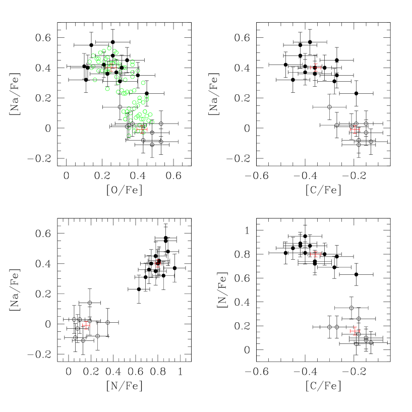
Figure 3: Correlation between light-elements (C,N,O,Na) as obtained from our GIRAFFE stars. Green points in the upper left panel are the results by Marino et al. (2008). N-poor stars are indicated as open circles, while N-rich as filled circles. Red crosses represent the mean value for each sub-population.

3 Abundance analysis

The chemical abundances for Na, Mg, Al, Si, Ca, Ti, Cr, Fe, and Ni were obtained from the equivalent widths (EWs) of the spectral lines. See Marino et al. (2008) for a more detailed explanation of the method we used to measure the EWs. For the other elements (Li, C, N, O, ¹²C/¹³C, Y, Ba, Eu), whose lines are affected by blending, we used the spectrum-synthesis method. For this purpose we calculated 5 synthetic spectra having different abundances for the element, and estimated the best-fitting value as the one that minimize the r.m.s. Na and Al present few features in the spectrum, so in this case abundances derived from the EWs were cross-checked with the spectral synthesis method in order to obtain more accurate measurements. Only lines not contaminated by telluric lines were used.

Atmospheric parameters were obtained in the following way. First of all T_eff was derived from the B-V color using the relation by Alonso et al. (1999) and the reddening (E(B-V)=0.36) from Harris (1996). Surface gravities (${\log(g)}$) were obtained from the canonical equation:

$$\log(\frac{g}{g_{\odot}})=\log(\frac{M}{M_{\odot}})+4\cdot\log(\frac{T_{\rm eff}}{T_{\odot}})-\log(\frac{L}{L_{\odot}})$$

where the mass ${M/M_{\odot}}$ was assumed to be 0.8 M_⊙, and the luminosity ${L/L_{\odot}}$ was obtained from the absolute magnitude ${M_{\rm V}}$ assuming an apparent distance modulus of ${(m-M)_{\rm V}}$=12.82 (Harris 1996). The bolometric correction (BC) was derived by adopting the relation BC-T_eff from Alonso et al. (1999). Finally, micro-turbulence velocity (${v_{\rm t}}$) was obtained from the relation of Marino et al. (2008).
These atmospheric parameters were considered as initial estimates and were refined during the abundance analysis. As a first step atmospheric models were calculated using ATLAS9 (Kurucz 1970) and assuming the initial estimate of T_eff, ${\log(g)}$, and ${v_{\rm t}}$, and the [Fe/H] value from Harris (1996).
Then T_eff, ${v_{\rm t}}$, and ${\log(g)}$ were adjusted and new atmospheric models calculated in an interactive way in order to remove trends in Excitation Potential (E.P.) and equivalent widths vs. abundance for ${T_{\rm eff}}$ and ${v_{\rm t}}$ respectively, and to satisfy the ionization equilibrium for ${\log(g)}$. FeI and FeII were used for this purpose. The [Fe/H] value of the model was changed at each iteration according to the output of the abundance analysis. The Local Thermodynamic Equilibrium (LTE) program MOOG (Sneden 1973) was used for the abundance analysis.

We checked the reliability of our atmospheric parameters by comparing photometric and spectroscopic T_eff, finding a mean difference in temperature lower than 50 K.
A further check was performed on our log(g) scale. We inverted the previous equation in order to obtain the mass and calculated the mean mass of our targets. We got $\overline{M}$$=0.83\pm 0.06\ M_{\odot}$, in good agreement with the value obtained from isochrone fitting ($\sim$0.8 M_⊙). Our conclusion is that our T_eff and log(g) values can be safely used to obtain abundances.

The linelists for the chemical analysis were obtained from many sources (Gratton et al. (2003), VALD & NIST, McWilliam & Rich (1994), McWilliam (1998), SPECTRUM, and SCAN), and calibrated using the Solar-inverse technique by the spectral synthesis method (see Villanova et al. 2009 for more details). For this purpose we used the high resolution, high S/N NOAO Solar spectrum (Kurucz et al. 1984). Adopted solar abundances we obtained with our linelist are reported in Tab. 3 and 4 together with those ones by Grevesse & Sauval (1998) for comparison. We emphasize the fact that all the linelists were calibrated on the Sun, including those used for the spectral synthesis.

Lines treated with the EQW method are reported in Tab. 6 (electronic edition) together with the adopted parameters and equivalent widths star-by-star. Parameters for lines treated with the spectral synthesis method are not reported because the line list would be too long (thousands of lines in some cases). For these lines references are given above.

Li was measured from the line at 6707 Å, while our determinations of C,N,O abundances are based on the G-band at 4310 Å, the CN band at 4215 Å, and the forbidden O line at 6300 Å respectively. CN lines at 4230 Å were used also to estimate the ¹²C/¹³C ratio.

These features were also checked on the high resolution, high S/N spectrum of Arcturus. See Villanova et al. (2010) for more details. Abundances for C, N, and O were determined all together in an interactive way in order to take into account any possible molecular coupling of these three elements.

Our targets are objects evolved off the main sequence, so some evolutionary mixing is expected. This can affect the primordial C,N,O abundances separately, but not the total C+N+O content because these elements are transformed one into the other during the CNO cycle. Is does not affect the relative C,N,O of our stars either, since the stars are all in the same evolutionary phase.

Na was obtained from lines at 6154 and 6160 Å (EQW) and 5682 and 5688 Å, and corrected for NLTE effects following the prescription by Gratton et al. (1999). Mg was obtained from the line at 5711 Å while Al from the lines at 6696 and 6699 Å. Y abundance was measured using the line at 4375 Å while for Ba we used the line at 6494 Å(see Fig. 2, left panels). For Ba we took the hyperfine splitting into account using McWilliam & Rich (1994) and McWilliam (1998) data. Finally Eu was obtained from the line at 6645 Å.

In order to extend and confirm our results, we analyzed also a subsample of 24 stars of Marino et al. (2008) observed with UVES, the high-resolution spectrograph mounted at VLT telescope. As parameters we used those published there, but we extended the chemical analysis to Y and Zr (see Fig. 2, right panels), two elements not considered in that paper. Y was obtained from the line at 4900 Å, while Zr from the line at 6127 Å. Also in this case abundances were obtained by spectrum-synthesis. In UVES spectra two other Y lines were available, at 4883 and 5087 Å, but the one at 4900 Å turned out to be stronger and less affected by noise. It is partially blended with another line as is visible in Fig. 2, but this can be easily managed by the spectrum-synthesis method we applied.

An internal error analysis was performed by varing T_eff, log(g), [Fe/H], and v_t and redetermining abundances of star #33584, assumed to represent the entire sample. Parameters were varied by $\Delta$T_eff=+50 K, $\Delta$log(g)=+0.10, $\Delta$[Fe/H]=+0.05 dex, and $\Delta$v_t=+0.1 km/s. This estimation of the internal errors for atmospheric parameters was performed as in Marino et al. (2008). Results are shown in Tab. 5, including the error due to the noise of the spectra. This error was obtained, for elements whose abundance was obtained by EQWs, as the average value of the errors on the mean as given by MOOG, and for elements whose abundance was obtained by spectrum-synthesis, as the error given by the fitting procedure. $\sigma_{\rm tot}$ is the squared sum of the single errors, while $\sigma_{\rm obs}$ is the mean observed dispersion of the two sub-populations of the clusters (as identified by their N content, see next section). The agreement between the two values is reasonable for all elements.

4 Results

First of all, in Fig. 3 we plot the abundance of C,N,O,Na. In all the panels we clearly see that the distribution is bimodal for all the four elements considered. Na-O anti-correlation is compared with Marino et al. (2008) (green points). We confirm that stars in the cluster are divided in two well separated groups having different light-element content. In the following analysis we take as reference the lower left panel of Fig. 3 because N appears to be the best element to separate the two groups. From now on in all the figures and in the discussion of the results, we divide our stars into N-poor (open circles in all the figures), and N-rich (filled circles in all the figures).

We note that in our sample 9 stars belong to the N-poor group (the so called first generation), while 14 to the N-rich group (the so called second generation). This means that about 40% of our stars belong to the first generation. This agree within the errors ($\sigma\sim\pm$6%) with Carretta et al. (2009) and Marino et al. (2008), where the authors find that the cluster is composed of $\sim$30% and $\sim$50%, respectively, first generation stars.

Errors on the single measurements (the black errorbars in the figures) for a given element are the $\sigma_{\rm obs}$ of Tab. 5. The red crosses in the figures represent the mean abundance and the error of the mean for each group. We see that N-poor stars are also C-rich, O-rich, and Na-poor, while N-rich stars are also C-poor, O-poor, and Na-rich, in accord with the theoretical expectations outlined previously.

Mean abundances we obtained for the two groups and for the cluster are summarized in Tab. 2, while abundances for each star are summarized in Tab. 3, and 4.

With respect to the mean abundances of the two groups, for each element in the 4^th colum of Tab. 2 we report the abundance difference (i.e. the significance) in units of $\sigma_{el}$ that is defined as:

$$\sigma_{el}=\sqrt{\sigma_{el,N-poor}^{2}+\sigma_{el,N-rich}^{2}}$$

where $\sigma_{el,N-poor}$ and $\sigma_{el,N-rich}$ are the errors on the mean abundance of the two groups as given by the 2^nd and 3^rd columns of Tab. 2. This value tell us if this difference is significant with a value of $\sigma_{el}>$3 implying strong significance. The second part of Tab. 4 reports the results obtained from the analysis of the UVES spectra of Marino et al. (2008). Na abundances are obtained from that paper. For these stars we do not have the N content. However it is clear from Fig. 3 that N-poor and N-rich stars can be easily identified also by their Na content. So UVES stars were classified according to their [Na/Fe] value. All stars with [Na/Fe]$<$0.23 were considered N-poor, all stars with [Na/Fe]$\geq$0.23 were considered N-rich.

Table 2: Mean abundances of the two groups of stars (2^nd and 3^rd column). The 4^th column is the the significance of the abundance difference of the two groups, in units if $\sigma_{el}$. 5^th column gives the mean abundance of the cluster as the average of the two groups. 6^th, 7^th, and 8^th columns are the abundances by Marino et al. (2008, Ma08), Ivans et al. (1999, Iv99), and Yong et al. (2008)+Yong et al. (2008b)=Yo08, respectively. The results of the last two papers are reported together because they are complementary.

El.	N-poor	N-rich	Sig. (units of $\sigma_{el}$)	M4(this work)	Ma08	Iv99	Yo08
GIRAFFE data
log$\epsilon$(Li)	+0.97$\pm$0.04	+0.97$\pm$0.03	0.0	+0.97	-	-	-
${\rm[C/Fe]}$	-0.20$\pm$0.02	-0.36$\pm$0.02	5.7	-0.28	-	-0.50	-
${\rm[N/Fe]}$	+0.16$\pm$0.03	+0.80$\pm$0.02	17.8	+0.48	-	+0.85	-
${\rm[O/Fe]}$	+0.42$\pm$0.03	+0.25$\pm$0.03	4.0	+0.34	+0.39	+0.25	+0.56
log$\epsilon$(C+N+O)	8.18$\pm$0.03	8.14$\pm$0.02	1.1	8.16	-	8.24	-
12C/13C	21.7$\pm$0.8	17.4$\pm$1.0	3.4	19.6	-	4.5	-
${\rm[Na/Fe]}$	-0.01$\pm$0.03	+0.40$\pm$0.02	11.4	+0.20	+0.27	+0.22	+0.43
${\rm[Mg/Fe]}$	+0.46$\pm$0.03	+0.48$\pm$0.02	0.5	+0.47	+0.50	+0.44	+0.57
${\rm[Al/Fe]}$	+0.51$\pm$0.04	+0.53$\pm$0.02	0.4	+0.52	+0.54	+0.64	+0.74
${\rm[Si/Fe]}$	+0.43$\pm$0.02	+0.42$\pm$0.02	0.4	+0.43	+0.48	+0.65	+0.58
${\rm[Ca/Fe]}$	+0.42$\pm$0.01	+0.40$\pm$0.02	0.9	+0.41	+0.28	+0.26	+0.42
${\rm[Ti/Fe]}$	+0.35$\pm$0.02	+0.31$\pm$0.01	1.8	+0.33	+0.32	+0.30	+0.41
${\rm[Cr/Fe]}$	+0.00$\pm$0.02	+0.01$\pm$0.03	0.3	+0.01	-0.04	-	+0.08
${\rm[Fe/H]}$	-1.14$\pm$0.01	-1.14$\pm$0.02	0.0	-1.14	-1.07	-1.18	-1.23
${\rm[Ni/Fe]}$	+0.00$\pm$0.01	-0.02$\pm$0.01	1.4	-0.01	+0.02	+0.05	+0.12
${\rm[Y/Fe]}$	+0.10$\pm$0.06	+0.31$\pm$0.03	3.1	+0.21	-	-	+0.69
${\rm[Ba/Fe]}$	+0.29$\pm$0.02	+0.32$\pm$0.01	1.3	+0.31	+0.41	+0.60	-
${\rm[Eu/Fe]}$	+0.20$\pm$0.03	+0.20$\pm$0.03	0.0	+0.20	-	+0.35	+0.40
UVES data
${\rm[Na/Fe]}$	+0.07$\pm$0.03	+0.42$\pm$0.02	9.7	+0.25	+0.27	+0.22	+0.43
${\rm[Y/Fe]}$	+0.19$\pm$0.03	+0.33$\pm$0.02	3.9	+0.26	-	-	+0.69
${\rm[Zr/Fe]}$	+0.44$\pm$0.02	+0.47$\pm$0.03	0.8	+0.46	-	-	+0.23

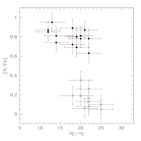
Figure 4: [N/Fe]-¹²C/¹³C anti-correlation for our GIRAFFE stars. Red crosses represent the mean value for each sub-population.

Comparing values in Tab. 2 we see immediately that the two sub-populations have the same content (difference of 1.8$\sigma$ in the worst case) of $\alpha$ (Mg,Si,Ca,Ti) and iron-peak (Cr,Fe,Ni) elements. Also the Li and Al abundances and the total C+N+O content are the same within the errors.

On the other hand the light elements C,N,O,Na are different between the two groups, with a significance of more than 4 $\sigma$. Also the carbon isotopic ratio is different. This is shown in Fig. 4, were we plot [N/Fe] vs. ¹²C/¹³C. In this figure an anti-correlation appears, and the difference in ¹²C/¹³C between the two groups is more than 3 $\sigma$, although there is a substantial overlap of the two distributions due in part to the measurement error. This result is not unexpected because the N-rich population is supposed to be born from material more chemically evolved with respect to the N-poor one. So it should have a lower carbon isotopic ratio, as we find.

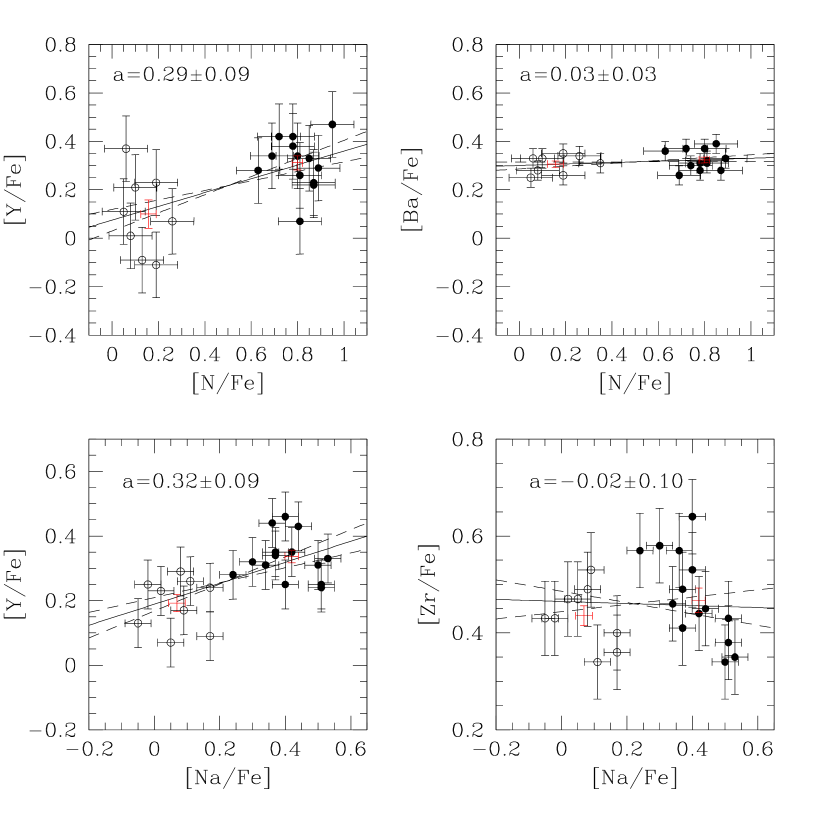
Figure 5: Upper panels: [Y/Fe] and [Ba/Fe] as a function of [N/Fe] for our GIRAFFE stars. Lower panels: [Y/Fe] and Zr/Fe as a function of [Na/Fe] for out UVES stars. A straight line was fit to the data of each panel and the slope with its error is reported. Red crosses represent the mean value for each sub-population.

Fig. 5 (upper panels) displays the abundances of the s-elements Y and Ba for our GIRAFFE data. As in the case of the $\alpha$ and iron-peak elements, the two sub-populations have the same Ba content. However the mean Y abundance is significantly different, at a level of more than 3 $\sigma$ (see Tab. 2). We fitted to the points a straight line and calculated the slope and its error. Values are reported inside each panel. The Ba slope is compatible with 0 (i.e. the same mean [Ba/Fe] value for the two groups), while the Y slope is incompatible with 0 with a confidence of more than 3 $\sigma$ (i.e. two different mean [Y/Fe] values for the two groups, although there is substantial overlap between the two distributions due in part to the measurement error). We cannot rule out a trend, but we favor a bimodality.

Lower panels display the abundances of the s-elements Y and Zr for the UVES data vs. [Na/Fe]. Again the mean Y content of Na-poor (N-poor) and Na-rich (N-rich) stars is very different, at a level of more than 3 $\sigma$, while they share the same Zr abundance.

The Y abundance from GIRAFFE and UVES observations deserves a further comment. For N-rich stars the two databases give very good agreement (+0.31 vs +0.33 dex), well within 1$\sigma$. Values for N-poor stars instead appear different ([Y/Fe]=+0.10$\pm$0.06 dex for GIRAFFE and [Y/Fe]=+0.19$\pm$0.03 dex for UVES). However if we consider the errors, the difference of 0.09 dex is significant at the level of 1.3 $\sigma$, too low to imply a real difference, so we can safely attribute it to measurement errors.

The total error on Y (0.12 dex, see Tab. 5) due to atmospheric parameters and S/N is high. It is dominated by errors in gravity and microturbulence, but also S/N gives a not-negligible contribution. However this is a random internal error, and for this reason it is fully included in the error of the mean Y abundance of the two groups of stars that we use to calculate the significance in Tab. 2.

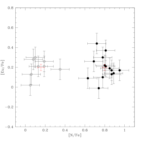
Figure 6: [Eu/Fe] vs. [N/Fe] for our GIRAFFE stars. Red crosses represent the mean value for each sub-population.

Finally in Fig. 6 we report [Eu/Fe] as a function of [N/Fe]. At odds with the Y-abundance discussed before, Eu does not show any trend, confirming the result reported in Tab. 2.

Thus, we find no significant difference between the two groups defined by their N (or Na) abundance, in Li,C+N+O,Mg,Al,Si,Ca,Ti,Cr,Fe,Ni,Zr,Ba or Eu, but find very significant differences in C,N,O,¹²C/¹³C,Na, and Y.

4.1 Comparison with literature

Firstly we compare our result with Marino et al. (2008) (see Fig. 3). Also in that case the authors find a bimodal Na-O anti-correlation. They define a Na-poor (green points with [Na/Fe]$\leq$0.25) and a Na-rich (green points with [Na/Fe]$>$0.25) population, which correspond to our N-poor and N-rich respectively. Their Na-rich population have the same mean Na content as our N-rich stars, while their Na-poor stars have a mean Na content that is slightly higher than that of our N-poor population. This could be a residual of the NLTE correction. Here we show that the bimodality is extended also to C, N,¹²C/¹³C, and Y. As Marino et al. (2008), we do not find bimodality in $\alpha$ (Mg,Si,Ca,Ti) or iron-peak elements(Cr,Fe,Ni), nor Ba. In particular Marino et al. (2008) Na-poor and Na-rich populations have the same [Ba/Fe] within 1 $\sigma$, confirming our finding. Thus the two populations have the same abundance as far as these elements are concerned.

Another important paper is Ivans et al. (1999). These authors include also N and indirectly C in their results. They find the same Na-O anticorrelation as we do (see their Fig. 14, upper panel). They find also a relatively well-defined C-O correlation and N-O anticorrelation as is implied also by our Fig. 3. Their C+N+O content is constant within the errors for all the stars, but a bit higher that our result (8.24 vs. 8.16 respectively) in absolute value. As in our case a bimodality is suggested by their measurement of the strength of the CN band at 7874 Å (see their Fig. 11), and partially visible in the N-O anticorrelation where a discontinuity at log$\epsilon$(N)$\sim$7.70-7.80 is visible.

As suggested by the referee, we comment in more detail on the Al content. Marino et al. (2008) found a possible spread in Al, confirmed by Ivans et al. (1999), where Al is correlated with Na with a significance of more than 3$\sigma$. We instead find that the Al content is the same for the two groups of stars, which implies no Al-Na correlation. A possible explanation could be the presence of some unrecognized molecular line (CN?) that is blended with Al lines. This line could preferentially affect colder stars, and both the Marino et al. (2008) and Ivans et al. (1999) stars are colder than ours. Because C and N have different abundances for the two groups, we expect that this hypothetical line has a different strength (assuming the same T_eff) if a star belongs to one group or the other. This would cause a spurious correlation between Al and N or Na also if the Al content is the same for the two groups. This hypothesis is not totally unreasonable because the spectral ATLAS of Arcturus shows that the Al lines are possibly blended with some CN line (i.e. the CN line at $\lambda$= 6698.746 Å), but the apparent lack of an increasing trend in Al abundance with evolutionary phase in previous works could argue against it.

Another explanation could be the evolutionary state of Marino et al. (2008) and Ivans et al. (1999) targets. Their stars are all above the RGB-bump and so affected by more evolutionary mixing. This is also proved by the ¹²C/¹³C value obtained by Ivans et al. (1999) that is of the order of 4-5. Our stars instead have ¹²C/¹³C$\sim$20, implying a less dramatic mixing. A deeper mixing after the RGB-bump could alter significatively (and differentially, with the N-rich group being the most affected) the primordial Al content through products of the MgAl-cycle. Howver if nucleosynthesis products of the MgAl-cycle are indeed mixed up at this evolutionary phase, this would have consequences also for the Na abundances, as the NeNa-cycle operates at lower temperatures (Charbonnel 2005), and there are studies that argue against such changes (Gratton et al. 2000). A further discussion of this point is beyond the scope of this paper. In any case, in the present paper we find that N-poor and N-rich stars have the same Al content.

Our main results are independent of the absolute abundances, but we want to add further comments on this point. Comparison with absolute abundances published by Marino et al. (2008), Ivans et al. (1999), Yong et al. (2008), and Yong et al. (2008b) (the four most recent papers) are reported in Tab. 2. The last two papers are reported as one (Yo08) in the table and in the following discussion because they are complementary. For some elements the mean abundance of the cluster agrees well (difference of 0.1 dex or less) with these four papers. This is true for C+N+O, Mg, Ti, Cr, and Fe. ¹²C/¹³C is higher in our case, as expected by the evolutionary stage of our stars. Our Al, Si, and Ba content agrees well also with Marino et al. (2008), but in this case the scatter is larger (between 0.1 to 0.3 dex) with respect to Ivans et al. (1999) and Yo08. Our [O/Fe], [Na/Fe], and [Ni/Fe] match Marino et al. (2008) and Ivans et al. (1999) within 0.1 dex, while the disagreement is worse (0.22, $\sim$0.2, and 0.13 dex respectivelly) with respect to Yo08. On the other hand our [Ca/Fe] matches Yo08, but it is 0.13 and 0.15 dex higher then Marino et al. (2008) and Ivans et al. (1999). The difference in C and Eu is a bit high (0.22 and 0.15 dex respectively) with respect to Ivans et al. (1999), but it is large (0.37 dex) only in the case of N. Finally Yo08 obtained a Zr value 0.23 dex lower than our, a Eu value 0.20 dex higher, while the disagreement is large as far as [Y/Fe] is concerned ($\sim$0.4$\div$0.5 dex).

We further comment about Ba and Eu. We find [Ba/Fe]$\sim$+0.3, in agreement with Marino et al. (2008) who give [Ba/Fe]$\sim$+0.4. Ivans et al. (1999) gives a much higher value ([Ba/Fe]$\sim$+0.6) while Gratton et al. (1986) gives [Ba/Fe]$\sim$+0.0. Our value is in the middle of the literature values. We find [Ba/Eu]=+0.10, lower than Ivans et al. (1999) but still higher than the solar system value and much higher then field halo and globular cluster giants, where [Ba/Eu] is typically negative with a range from -0.2 to -0.6 (Ivans et al. 1999). This result confirms that M4 has a larger s- to r-process contribution than in the Sun, and also supports the Ivans et al. (1999) suggestion that the period of star formation and mass loss that preceded the formation of the observed stars in M4 was long enough for AGB stars to contribute their ejecta into the primordial ISM of the cluster.

5 Discussion

As discussed in the introduction, all GCs studied in detail to date show some kind of spread in their light-element (from C to Al) abundance. The amount of the spread varies a lot from cluster to cluster. Some GCs, such as M22 (Marino et al. 2009), show also a spread in $\alpha$ and iron-peak elements, but this is an uncommon feature. So in this discussion we consider only M4-like objects, i.e. those clusters having only a spread in light elements (and possibly in s-elements). However M4 appears to be rather unique in that the ’spread’ is actually a bimodality.

The most natural explanation for this phenomenon is the self-pollution scenario, where a first generation of stars is formed from primordial material. In the most accepted model, this material is O-rich and Na-poor with respect to the second generation that will form later. Then some class of stars (massive MS stars, either fast rotating or binaries, or intermediate-mass AGB stars) of this first generation pollute the interstellar material. This material (O-poor and Na-rich) is kept in the cluster due to the strong gravitational field of the massive cluster, and it gives rise to a new generation of stars. In this model the O-rich/Na-poor stars are the oldest. Also the abundance of other elements (including He or other light and s-process elements) may differ in stars of the first and second generation.

Another scenario postulates instead that the primordial material the first generation will form from is O-poor and Na-rich because of initial pollution by SNeIa and AGB stars. Then SNeII of the first generation explode polluting the residual material, and a second generation is formed, being O-rich and Na-poor. The final result is the same, but in this case the O-poor/Na-rich stars are the oldest.

Each one of these polluters has its own chemical signature as discussed in the introduction. SNeII ejects material that is strongly $\alpha$-enhanced but only slightly enhanced in iron-peak elements. The Marcolini et al. (2009) scenario manages to produce a second generation that has the same iron-peak element content as the first generation because of the mix with primordial Fe-poor material. Nothing is said in that paper about $\alpha$-elements with the exception of O and Mg. However the first generation is poor in $\alpha$-elements (Si,Ca,Ti) because it is formed from material polluted by SNeIa and AGBs (that do not produce these elements or only in a negligible amount), while the second generation must be rich in $\alpha$-elements (Si,Ca,Ti) both because of the contamination by the SNeII of the first generation, but also because of the mix with primordial material that was pre-contaminated by previous SNeII.

The exact estimation of the difference in Si,Ca,Ti content is beyond the purpose of this paper, but we can give a rough number. In Marcolini et al. (2009, Tab. 1) we can see that the progenitor material of the first generation is enhanced by $\sim$1 dex in its Fe content with respect to the primordial one, due to the SNIa explosion. So the material the first generation will form from is dominated by the products of the SNIa ejecta (plus the AGB ejecta, that however do not affect Si,Ca,Ti content). The second generation instead is formed from material whose abundance ratio is dominated by SNeII ejecta. So we can estimate the difference in Si,Ca,Ti between the two generations comparing the Si,Ca,Ti content of Galactic stars with [Fe/H]$\leq$-1.0 dex, whose abundance ratio is dominated by SNeII ejecta, and stars with [Fe/H]$\sim$0.0, whose abundance ratio is dominated by SNeIa ejecta. According to Pompeia et al. (2008, Fig. 8), the difference of the order of $\Delta$[Si,Ca,Ti/Fe]$\sim$0.3. This is our reference value. Because SNeII produce also r-element (i.e. Eu), the second generation should be also Eu-enhanced.

AGB stars are the main producers of s-elements, including both light-s such as Y, Zr, and heavy-s like Ba, through the main component of the s-process.

Massive MS stars (M$>$15M_⊙, both as fast rotators or in binary systems) produce only light s-elements (e.g. Y) through the weak-s process but not heavy s-elements.

We now compare these predictions with our observational results. N-poor and N-rich stars have the same Si,Ca,Ti content within a few hundredths of a dex. They also share the same Eu abundance. According to these results and comparing them with the Si,Ca,Ti content expected from Marcolini et al. (2009) scenario, SNeII are not viable candidates for the polluters responsible.

The two groups also have the same Ba content, suggesting that AGB stars cannot be responsible for the pollution. This statement is reinforced if we compare our results with theoretical predictions. Considering both GIRAFFE and UVES databases, we have a difference in [Y/Fe] for the two groups of stars of 0.18 dex. According to Busso et al. (2001) or the more recent paper by Karakas et al. (2010), we would have expected to see an equal (if not larger) difference in [Ba/Fe], assuming AGB stars as polluters. And we have the observational counterpart of that. NGC1851 (Villanova et al. 2010) hosts two distinct populations that differ in [Y/Fe] at the level of 0.11 dex. They have a difference in [Ba/Fe] that is much larger, 0.41 dex. So for NGC1851 we can postulate AGBs as the most probable polluters, while for M4 it is very unlikely.

We are left with massive MS stars. These objects should pollute the interstellar material with light s-elements (besides C,N,O,Na,Al) produced through the weak s-process. We found that the two populations differ in their Y content at a level of more than 3 $\sigma$, but they have the same Zr content. This results fits with the theoretical scenario (Raiteri et al. 1993; Travaglio et al. 2004) that says that the weak s-component is responsible for a major contribution to the s-process nuclides up to A$\sim$90 with a peak for A=80 (⁸⁰Kr). The last nuclide of the chain is uncertain due to the many theoretical uncertainties, but it is not unreasonable (and it is compatible with the models) to postulate that, according to our results, the last nuclide produced in a significant amount is ⁸⁹Y, leaving the next nuclide, ⁹⁰Zr, and heavier s-elements, relatively scarce. Unfortunately we cannot measure s-elements lighter then Y (i.e. Rb or Sr) in order to further investigate our statement. However we can obtain an important confirmation from Yong et al. (2008b). These authors estimated Na, Rb, Y, and Pb for a sample of targets, and their results are reported in Fig. 7 for those stars with all three elements measured. First of all also in this case Na appears to be bimodal, with a gap between 0.2$<$[Na/Fe]$<$0.4. But, most important, both Y and Rb appear to have a positive trend with Na (or N), exactly as we have found (but only for Y). This would confirm that light s-elements like Y or lighter have a different mean abundance in the two populations of M4. The trends, taken separately, have a significance of only 1.2$\div$1.3 $\sigma$, as shown in Fig. 7, but if we compare the mean Rb content of the two groups (red crosses in Fig. 7, lower panel) that are of +0.37$\pm$0.02 and +0.42$\pm$0.02 respectively, we have a significance of 1.8 $\sigma$. We obtain an even stronger confirmation if we consider the two trends together and apply the following ab absurdum argument. Let’s assume that our previous result is wrong and that the two populations have the same Rb and Y content. With this hypothesis and using the Kolmogorov-Smirnov test, the probability of having a Y vs. Na data distribution like that one in Fig. 7 is 17%. For the Rb vs. Na data distribution we have a probability of 9%. These two values match with the significance at 1.2$\div$1.3 $\sigma$ found above. Under the previous hypothesis the relations visible in Fig. 7 would be due only to measurement errors, so they would be independent and we can calculate the probability of having both relations we see in Fig. 7 by multiplying the two individual values. The final result is only 1.5%. So the probability of the initial hypothesis to be true is only 1.5%. This means that Yong et al. (2008b) confirms our result of a bimodality in light s-elements with a confidence level of 98.5%. Another hint comes from Pb. This is a pure s-element, produced only in AGB stars (Travaglio et al. 2004). The mean [Pb/Fe] abundances of the two Na groups in Yong et al. (2008b) are +0.26$\pm$0.05 and +0.31$\pm$0.02 respectivelly. In this case the significance is 0.8 $\sigma$. This further rules out AGB stars as candidate polluters, in agreement with our statement based on Ba. Because of this and because we have double-checked with two different spectrographs and two different lines the Y-bimodality, we are led to the conclusion that the best candidates for the Y-enrichment for the second generation in M4 is the weak s-process, which implies that massive (M$>$15 M_⊙) MS stars are the best candidates for the self-pollution scenario.

A further conclusion can be obtained from Mg and Al. These elements are processed in the Mg-Al cycle where Al is produced at the expense of Mg. The fact that we find the same Mg and Al abundance for N-poor and N-rich stars implies that the Mg-Al cycle did not activate, at least in the ejected material responsible for the pollution. This implies an upper limit for the temperature: the material burns at a temperature lower than 50$\times$10⁶ K (Decressin et al. 2007). This implies also that the massive stars responsible for the pollution must have been less massive than 60 M_⊙. Another hint comes from the difference in the mean [O/Na] value of the two groups. In our database it is of the order of 0.7 dex, while Marino et al. (2008) give 0.5 dex, so we assume a mean value of 0.6 dex. Decressin et al. (2007) (see their Fig. 10) give the extension of the [O/Na] distribution as a function of the mass of the polluter. 0.6 dex implies a mass higher then 20 M_⊙ but significantly lower than 30 M_⊙. A value between 20 and 30 M_⊙ seems reasonable.

Our conclusion is that the best candidate in order to explain the abundance spread in M4 are massive MS stars (fast rotators or binaries) with masses of the order of 20$\div$30 M_⊙. Interestingly enough, there is another cluster with the same chemical signature as M4, that is NGC 6397, recently investigated by Lind et al. (2011). In that paper the authors find a bimodality in Na for the cluster as in M4, but also a difference in [Y/Fe] between the two sub-populations at a level of almost 3$\sigma$. As in our case the content of the other neutron-captured elements (Zr,Ba,Ce,Nd,Eu), all heavier than Y, is the same within $\sim$1$\sigma$. They say that the [Y/Fe] differecence is ’too small to be convincing’ (citation), but in the view of our result it could be real. Based on the abundance pattern, they support the MS massive star scenario too. These findings suggest also the hypothesis that a bimodality in light-elements (C,N,O,Na) could be a normal feature of the MS massive star based self-pollution scenario.

We underline the fact that our conclusion is valid for M4 (and possibly NGC 6397). Other clusters show a Mg-Al anticorrelation or light and heavy s-element spread (i.e. NGC 1851, Villanova et al. 2010), so AGB stars can be involved.

Finally some clusters like $\omega$ Centauri or M22 have a spread in Ca and Fe, so SNeII must also be at work. The picture is that each cluster may have its own peculiar process of formation within the pollution scenario, and that the polluters can be different.

A peculiarity of M4 is its bimodal distribution, at odds with many other clusters where the Na-O anticorrelation is continuous (Carretta et al. 2009). This implies that the clusters had a first star forming burst followed by a quiescent period, where processed material started to flow and mix with the primordial gas. During this period no star was formed and the gas had time to homogenize, otherwise we would have observed a continuous anticorrelation as in the other clusters. After that, a second burst happened with the formation of the second generation. The exact time scale of this process is unknown. However it must have been longer than the evolutionary time of very massive stars (some Myrs), but shorter than the evolutionary time of AGB stars ($\geq$40 Myrs, Ventura & D’Antona 2009). For the 20$\div$30 M_⊙ star polluters postulated above, the evolutionary timescale is of the order of $\sim$10$\div$30 Myrs.

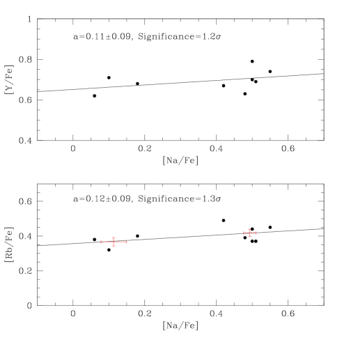
Figure 7: [Y/Fe] vs. [Na/Fe] and [Rb/Fe] vs. [Na/Fe] for stars from Yong et al. (2008b). Linear fits and the slopes with their significance (in units of $\sigma$) are reported. For [Rb/Fe] vs. [Na/Fe] we plotted the mean abundances (red crosses) of the two groups of Na-poor ([Na/Fe]$<$0.30 dex) and Na-rich ([Na/Fe]$>$0.30 dex) stars.

6 Conclusions

In this paper we analyzed a sample of 23 stars belonging to the RGB of M4 (NGC 6121) and observed with the GIRAFFE@FLAMES spectrograph. Our targets are located below the RGB bump. We complemented our study by analyzing a subsample of UVES@FLAMES spectra of Marino et al. (2008). We estimated abundances for many key elements: Li,C,N,O,¹²C/¹³C,Na,Mg,Al,Si,Ca,Ti,Cr,Fe,Ni,Zr,Y,Ba,Eu. Our aim was to look for some hint in order to help solve the problem related to the self-pollution scenario in GCs. According to this scenario, a cluster experiences an extended period of star formation, where the younger populations were born from an interstellar medium polluted by products of the CNO, NeNa, and MgAl cycles coming from massive stars of the former generation. Postulated polluters include: massive MS stars (M$>$15 M_⊙, fast rotating or binaries), intermediate mass AGB stars (4$<$M$<$7 M_⊙), or SNeII. Each of these candidates has its own unique chemical signature. We confirm the presence of a bimodal population, where the two groups of stars can easily be separated by their N content. One group (presumably the oldest generation) is N-poor, while the other (the younger generation) is N-rich. N-poor and N-rich stars have significantly different C,N,O,¹²C/¹³C,Na, and Y content, but share the same Li,C+N+O,Mg,Al,Si,Ca,Ti,Cr,Fe,Ni,Zr,Ba, and Eu abundances. This rules out SNeII because they would produce a second generation $\alpha$-enhanced with respect to the first one (and Eu enhanced). AGB stars are also excluded because they should produce a Zr and Ba-enhanced (in addition to Y-enhanced) second generation through the main s-process. We are left with massive MS stars. These objects are able to produce the difference in light elements we observe but, most important, they can produce also light s-elements like Y through the weak s-process. The Y-enhancement of the second generation is the most interesting result we found. This scenario is supported also by Yong et al. (2008b). Based in this paper we found that the two M4 groups have different Rb content (that confirms massive MS stars as polluters) but the same Pb content (that further excludes AGB stars as polluters). The lack of Mg/Al enhancement and the extension of [O/Na] ratio points toward massive stars with 20$<$M$<$30 M_⊙ as the most likely polluters.

Our conclusion is that massive stars in the range 20$<$M$<$30 M_⊙ are responsible for the bimodal population in M4. The time scale for the formation of the clusters is $\sim$10$\div$30 Myrs, with two well separated bursts that generated a bimodal population. Other cluster have different chemical characteristics, so other kinds of polluters and star formations histories are required.

Table 3: Individual abundances (light, $\alpha$, iron-peak elements) of the observed GIRAFFE stars.

ID	log$\epsilon$(Li)	[C/Fe]	[N/Fe]	[O/Fe]	[Na/Fe]	[Mg/Fe]	[Al/Fe]	[Si/Fe]	[Ca/Fe]	[Ti/Fe]	[Cr/Fe]	[Fe/H]	[Ni/Fe]	12C/13C
28590	1.02	-0.42	0.89	0.26	0.48	0.48	0.66	0.38	-	0.26	-	-1.21	-0.05	18
33584	0.94	-0.21	0.35	0.34	0.01	0.54	0.64	0.45	0.41	0.31	-	-1.14	-0.04	20
36820	0.77	-0.27	0.78	0.34	0.45	0.49	0.64	0.49	0.42	0.32	0.10	-1.25	-0.02	20
37614	1.08	-0.18	0.26	0.43	-0.08	-	0.62	0.50	0.36	0.34	0.02	-1.16	0.04	22
39100	0.97	-0.19	0.05	0.37	0.03	0.42	0.44	0.47	0.40	0.36	-0.03	-1.08	0.00	25
40197	0.97	-0.27	0.78	0.40	0.35	0.51	0.51	0.51	0.42	0.28	-0.06	-1.14	-0.03	22
41863	0.91	-0.38	0.87	0.26	0.57	0.51	0.61	0.48	-	0.23	0.18	-1.19	-0.03	21
42561	0.96	-0.40	0.95	0.28	0.37	-	0.62	0.39	0.41	0.31	-0.06	-1.20	0.04	13
43020	1.05	-0.19	0.63	0.45	0.23	0.47	0.49	0.51	0.50	0.28	0.01	-1.12	-0.04	22
43085	1.01	-0.32	0.80	0.31	0.40	0.47	0.50	0.42	0.33	0.27	-0.05	-1.08	0.02	19
43494	0.93	-0.18	0.13	0.48	-0.11	0.49	0.31	0.43	0.44	0.31	0.00	-1.14	-0.05	22
43663	1.00	-0.28	0.69	0.30	0.31	0.36	0.43	0.45	0.33	0.30	0.06	-1.11	-0.07	19
45171	0.80	-0.13	0.06	0.53	-0.09	0.32	0.44	0.40	0.44	0.38	-0.09	-1.11	0.00	21
45200	0.94	-0.42	0.87	0.14	0.55	0.51	0.57	0.46	0.39	0.36	0.07	-1.12	0.00	12
46201	0.94	-0.40	0.81	0.10	0.41	0.54	0.55	0.31	0.44	0.34	-0.04	-1.17	-0.04	20
47596	1.00	-0.15	0.08	0.48	-0.03	0.44	0.54	0.35	0.42	0.31	0.04	-1.16	-0.02	22
48499	1.17	-0.15	0.10	0.53	0.03	0.47	0.60	0.54	0.47	0.39	-0.03	-1.15	0.04	25
49381	0.95	-0.27	0.19	0.35	0.02	0.59	0.47	0.38	0.45	0.42	0.13	-1.19	0.01	18
50032	1.02	-0.45	0.85	0.11	0.32	0.43	0.50	0.43	0.33	0.33	-	-1.04	0.01	12
53602	1.14	-0.36	0.72	0.23	0.36	0.36	0.39	0.37	0.45	0.33	-0.11	-1.03	-0.01	18
67553	0.90	-0.30	0.19	0.30	0.14	0.39	0.49	0.35	0.39	0.29	-0.05	-1.16	0.04	20
8460	0.99	-0.36	0.74	0.12	0.40	0.50	0.50	0.37	0.41	0.40	-	-1.16	-0.04	14
907	0.81	-0.48	0.81	0.21	0.42	0.56	0.46	0.37	0.42	0.31	0.03	-1.20	-0.03	14
Sun:our linelist
	-	8.49	7.95	8.83	6.32	7.56	6.43	7.61	6.39	4.94	5.63	7.50	6.26	-
Sun:Grevesse & Sauval (1998)
	-	8.52	7.92	8.83	6.33	7.58	6.47	7.55	6.36	5.02	5.67	7.50	6.25	-

Table 4: Individual abundances (s and r elements) of the observed GIRAFFE and UVES stars. For UVES also Na abundances from Marino et al. (2008) are reported.

GIRAFFE
ID	[Y/Fe]	[Ba/Fe]	[Eu/Fe]
28590	0.29	0.33	0.14
33584	-	0.31	0.18
36820	0.38	0.31	0.30
37614	0.07	0.34	-
39100	0.11	0.25	0.02
40197	0.42	0.28	0.10
41863	0.23	0.28	0.17
42561	0.47	-	0.17
43020	0.28	0.36	0.09
43085	0.34	0.37	0.22
43494	-0.09	-	0.21
43663	0.34	0.26	0.26
45171	0.37	0.33	0.13
45200	0.22	-	0.13
46201	0.07	0.32	0.21
47596	0.01	0.28	0.28
48499	0.21	0.33	0.30
49381	-0.11	0.26	0.21
50032	0.33	0.39	0.19
53602	0.42	0.37	0.44
67553	0.23	0.35	0.26
8460	-	0.30	-0.01
907	0.26	0.31	0.37
Sun:our linelist
	2.25	2.34	0.52
Sun:Grevesse & Sauval (1998)
	2.24	2.13	0.51
UVES
ID	[Na/Fe]	[Y/Fe]	[Zr/Fe]
19925	0.51	0.43	0.24
20766	0.53	0.35	0.33
21191	0.51	0.38	0.25
21728	0.37	0.41	0.35
22089	0.50	0.34	0.31
24590	0.30	0.58	0.32
25709	0.34	0.46	0.31
26794	0.36	0.57	0.44
27448	0.11	0.34	0.26
28103	0.17	0.40	0.09
28356	0.37	0.49	0.34
28797	0.44	0.45	0.43
28847	0.08	0.49	0.29
28977	0.40	0.64	0.46
29027	0.02	0.47	0.23
29065	0.17	0.36	0.24
29222	0.24	0.57	0.28
29272	0.05	0.47	0.07
29282	0.42	0.44	0.35
29545	-0.02	0.43	0.25
29598	0.40	0.53	0.25
29848	0.09	0.53	0.17
30209	-0.05	0.43	0.13
Sun:our linelist
	6.32	2.25	2.56
Sun:Grevesse & Sauval (1998)
	6.33	2.24	2.60

Table 5: Estimated errors on abundances due to errors on atmospheric parameters and to spectral noise compared with the observed errors

ID	$\Delta$Teff=+50 K	$\Delta$log(g)=+0.10	$\Delta$[Fe/H]=+0.05	$\Delta$vt=+0.10 km/s	S/N	$\sigma_{\rm tot}$	$\sigma_{\rm obs}$
$\Delta$(log$\epsilon$(Li))	+0.05	0.00	0.00	0.00	0.07	0.09	0.10
$\Delta$([C/Fe])	-0.02	0.01	0.03	0.03	0.05	0.07	0.07
$\Delta$([N/Fe])	0.05	0.01	0.02	0.03	0.05	0.08	0.09
$\Delta$([O/Fe])	-0.04	0.08	0.01	0.03	0.06	0.11	0.10
$\Delta$([Na/Fe])	-0.02	0.00	0.00	0.02	0.08	0.08	0.08
$\Delta$([Mg/Fe])	-0.02	-0.02	0.01	0.00	0.08	0.09	0.07
$\Delta$([Al/Fe])	-0.02	0.01	0.00	0.03	0.07	0.08	0.09
$\Delta$([Si/Fe])	-0.04	0.02	0.01	0.02	0.06	0.08	0.06
$\Delta$([Ca/Fe])	0.00	0.00	0.00	0.01	0.04	0.04	0.04
$\Delta$([Ti/Fe])	0.02	0.00	0.00	0.01	0.03	0.04	0.04
$\Delta$([Cr/Fe])	0.00	0.00	0.00	0.02	0.07	0.07	0.08
$\Delta$([Fe/H])	+0.05	-0.01	-0.01	-0.03	0.01	0.06	0.05
$\Delta$([Ni/Fe])	-0.01	0.01	0.00	0.01	0.03	0.03	0.03
$\Delta$([Y/Fe])	-0.03	0.06	0.01	-0.08	0.06	0.12	0.14
$\Delta$([Ba/Fe])	-0.02	0.03	0.03	-0.02	0.04	0.06	0.04
$\Delta$([Eu/Fe])	-0.05	0.04	0.01	0.03	0.07	0.10	0.10
$\Delta$(12C/13C)	0	0	0	0	3	3	4

Table 6: Equivalent Widths. Table 6 is published in its entirety in the electronic edition of the Journal.

Wavelength(Å)	Element	E.P.(eV)	log(gf)	#28590
5711.083	12.0	4.34	-1.67	86.4
6696.014	13.0	3.14	-1.56	34.7
6698.663	13.0	3.14	-1.83	14.3
5645.603	14.0	4.93	-2.12	23.6
5690.419	14.0	4.93	-1.84	35.0
5793.066	14.0	4.93	-2.02	28.4
6125.014	14.0	5.61	-1.58	14.3
6145.010	14.0	5.61	-1.45	20.7
6244.465	14.0	5.62	-1.34	23.9
6161.287	20.0	2.52	-1.29	54.3
6162.170	20.0	1.90	0.46	170.9
6166.429	20.0	2.52	-1.14	53.2
6126.214	22.0	1.07	-1.36	26.8
6258.098	22.0	1.44	-0.34	49.7
6261.094	22.0	1.43	-0.44	42.4