Abstract

Fermion mixing is generally believed to be a low-energy manifestation of an underlying theory whose energy scale is much larger than the electroweak scale. In this paper we investigate the possibility that the parameters describing lepton mixing actually arise from the low-energy behavior of the neutrino interacting fields. In particular, we conjecture that the measured value of the mixing angles for a given process depends on the number of unobservable flavor states at the energy of the process. We provide a covariant implementation of such conjecture, draw its consequences in a two neutrino family approximation and compare these findings with current experimental data. Finally we show that this infrared origin of mixing will be manifest at the Ice Cube DeepCore array, which measures atmospheric oscillations at energies much larger than the tau lepton mass; it will hence be experimentally tested in a short time scale.

1 Introduction

Mixing of elementary fermions is very well established from the experimental point of view [1] although the origin of the parameters that describe the quark [2] and lepton [3] mixing matrix remains a deep mystery in modern particle physics. Since the Standard Model (SM) is probably an effective theory up to some energy scale, above which new physics has to be accounted for, it is likely that flavor mixing has an ultraviolet origin, too. In fact, it is commonly believed that flavor mixing is a manifestation of an underlying theory whose energy scale resides well above the electroweak scale $v=(G_{F}\sqrt{2})^{-1/2}$. In this framework, the peculiar structure of the mixing matrices and, in particular, the striking difference between quark and lepton mixing can shed light on the symmetries of the underling theory [4], even if its energy scale is unattainable by high-energy accelerators [5, 6].

Though the ultraviolet origin remains the most plausible explanation of fermion mixing, in this paper we follow a different path and we consider that mixing might arise as a consequence of the low energy behavior of the interacting fermion fields. More precisely, we decouple the problem of the origin of the mass from the problem of flavor mixing assuming that the former is due to an ultraviolet mechanism (as the Higgs mechanism with diagonal Yukawa couplings) while the latter arises at energies $\ll v$ (“infrared origin”).

We are driven in such consideration by a few reasons. Firstly, an infrared origin can naturally produce opposite mixing structures between quark and leptons, since the low-energy behavior of the corresponding interacting fields is very different. It can also explain the persistent difficulties in linking the concept of “flavor neutrino states” to the standard properties of Fock states in quantum field theory (QFT) [7]. Even more, experimental neutrino data show intriguing features when interpreted not only as a function of the energy and source-to-detector baseline but also of the number of kinematic thresholds ($N$) for lepton production that the neutrino is able to cross.

The core of this paper is a conjecture that links the number of unobservable flavor states for a given process (3-$N$ if we assume the standard 3-family scenario) to the measured value of the mixing angle for such process. This conjecture is discussed and stated in the standard QFT framework in Sec. 2. A consistent implementation of the conjecture, which allows extracting specific predictions on neutrino mixing, is developed in Sec. 3. Phenomenological implications, especially for the Ice Cube DeepCore array [8], and comparison with existing data are presented in Sec. 4 and summarized in the Conclusions (Sec. 5).

2 Flavor projectors

The Standard Model and the Minimally Extended SM do not make predictions on the values of the elementary fermion masses and their mixing parameters (angles and CP violating phases). However, they entangle the problem of fermion mass generation with mixing through the Higgs mechanism. Indeed, the Higgs-fermion Yukawa Lagrangian of the Minimally Extended SM reads, in unitary gauge:

$$\mathcal{L}_{H,F} = -\frac{v+H}{\sqrt{2}}\left[\sum_{\alpha,\beta=d,s,b}Y^{\prime D}_{\alpha\beta}\overline{q^{\prime D}_{\alpha L}}q^{\prime D}_{\beta R}+\sum_{\alpha,\beta=u,c,t}Y^{\prime U}_{\alpha\beta}\overline{q^{\prime U}_{\alpha L}}q^{\prime U}_{\beta R}+\right.$$ (1)

$$\left.\sum_{\alpha,\beta=e,\mu,\tau}Y^{\prime D}_{\alpha\beta}\overline{q^{\prime D}_{\alpha L}}q^{\prime D}_{\beta R}+\sum_{\alpha,\beta=\nu_{e},\nu_{\mu},\nu_{\tau}}Y^{\prime D}_{\alpha\beta}\overline{q^{\prime U}_{\alpha L}}q^{\prime U}_{\beta R}\right]+H.c.$$

where $U$ and $D$ labels the up-type and down-type fermions $q^{\prime}$; L, R their chirality and $H$ the Higgs field; the Yukawa matrices $Y^{\prime}_{\alpha\beta}$ are generic $3\times 3$ matrices that can be diagonalized by biunitary transformations. No experiment has direct access to the Higgs-fermion couplings and, actually, the Higgs sector has not been established, yet; hence the only source of observables to discriminate weak flavor eigenstates from mass eigenstates remains charged-current (CC) interactions. In the SM (for quarks) and in the Minimally Extended SM (for quarks and leptons), the fact that CC interactions are the only source of flavor projectors is both due to flavor independence of e.m. + strong interactions and to the effectiveness of the GIM mechanism. In CC, the matrices that diagonalize the left-handed and right-handed, up-type and down-type fermions ($V_{L}^{U\dagger}$, $V_{R}^{U\dagger}$, $V_{L}^{D\dagger}$ and $V_{L}^{D\dagger}$) appear only in the combination $U=V_{L}^{U\dagger}V_{L}^{D}$, where $U$ indicates the CKM matrix for quark and the Pontecorvo-Maki-Nakagawa-Sakata (PMNS) matrix for leptons. For the neutral current (NC) part of the Lagrangian, the corresponding combinations are $V_{L}^{U\dagger}V_{L}^{U}=V_{D}^{U\dagger}V_{D}^{U}=V_{R}^{U\dagger}V_{R}^{U}=V_{R}^{U\dagger}V_{R}^{U}=1{\rm I}$. As a consequence, in the NC sector, the CKM and PMNS matrices are unphysical and the theory is symmetric under flavor exchange. It means, for instance, that a NC scattering amplitude is the same for any transformation $\alpha\rightarrow\beta$ that changes the flavor label of the neutrino ($\alpha=e,\mu,\tau$). This is equivalent to the usual statement that NC processes are flavor-independent.

Alternatively, we can re-state the previous result saying that, in the Minimally Extended SM, the removal of all flavor projectors (CC interactions) restores flavor symmetry since the corresponding quantum number becomes unphysical. This is the statement we want to broaden beyond the limit of applicability of the Minimally Extended SM.

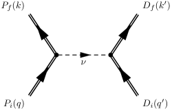
Figure 1: Feynman diagram that describes production, propagation and detection of a neutrino as a single process.

In order to do so, we assume without loss of generality [10, 11] that the process under consideration involves one initial state and one final state particle besides the neutrino and we employ the standard QFT formalism: hence, production, propagation and detection are considered simultaneously through the diagram of Fig.1. Following [10], we therefore define the states describing the particles accompanying neutrino production and detection as:

$$|P_{i}\rangle=\int\![dq]\,f_{Pi}(\vec{q},\vec{Q})\,|P_{i},\vec{q}\rangle\,,\qquad|P_{f}\rangle=\int\![dk]\,f_{Pf}(\vec{k},\vec{K})\,|P_{f},\vec{k}\rangle\,,$$ (2)

and

$$|D_{i}\rangle=\int\![dq^{\prime}]\,f_{Di}(\vec{q}^{\prime},\vec{Q}^{\prime})\,|D_{i},\vec{q}^{\prime}\rangle\,,\qquad|D_{f}\rangle=\int\![dk^{\prime}]\,f_{Df}(\vec{k}^{\prime},\vec{K}^{\prime})\,|D_{f},\vec{k}^{\prime}\rangle\,.$$ (3)

For any momentum label of Fig. 1, we shortened the notation defining

$$[dp]\equiv\frac{d^{3}p}{(2\pi)^{3}\sqrt{2E_{A}(\vec{p})}}\,.$$ (4)

In the formulas above, $|A,\vec{p}\rangle$ is the one-particle momentum eigenstate corresponding to momentum $\vec{p}$ and energy $E_{A}(\vec{p})$, and $f_{A}(\vec{p},\vec{P})$ is the momentum distribution function with $\vec{P}$ as mean momentum. Through the use of $f_{A}(\vec{p},\vec{P})$ we are aiming at computing the amplitude of Fig. 1 employing an external wave packet approach [11, 12, 13]. The main advantage of this approach is that it allows for a perturbative evaluation of the transition amplitude without resorting to the definition of “flavor states”. To see this, we first note that the amplitude of the Feynman diagram of Fig. 1 is given by:

$$i{\cal A}_{\alpha\beta}=\langle P_{f}\,D_{f}|\hat{T}\exp\Big{[}-i\int\!d^{4}x\,{\cal H}_{I}(x)\Big{]}-1{\rm I}|P_{i}\,D_{i}\rangle\,,$$ (5)

where $\hat{T}$ is the time ordering operator and ${\cal H}_{I}(x)$ is the CC weak interaction Hamiltonian, i.e. the part of the Hamiltonian that generates the flavor projectors for the process under consideration.

Eq.5 can be written explicitly as [10]:

$$i{\cal A}_{\alpha\beta} = \sum_{j}U_{\alpha j}^{*}U_{\beta j}\int\![dq]\,f_{Pi}(\vec{q},\vec{Q})\int\![dk]\,f^{*}_{Pf}(\vec{k},\vec{K})$$ (6)

$$\times\int\![dq^{\prime}]\,f_{Di}(\vec{q}^{\prime},\vec{Q}^{\prime})\int\![dk^{\prime}]\,f^{*}_{Df}(\vec{k}^{\prime},\vec{K}^{\prime})\,i{\cal A}^{p.w.}_{j}(q,k;q^{\prime},k^{\prime})\,.$$

The formalism is built in such a way that all intermediate states over which the sum is running are actually neutrino mass eigenstates, not flavor eigenstates. On the technical side, the quantity ${\cal A}^{p.w.}_{j}(q,k;q^{\prime},k^{\prime})$ is the plane-wave amplitude of the process with the $j$th neutrino mass eigenstate propagating between the source and the detector:

$$i{\cal A}^{p.w.}_{j}(q,k;q^{\prime},k^{\prime})= \int d^{4}x_{1}\!\int d^{4}x_{2}\,\tilde{M}_{D}(q^{\prime},k^{\prime})\,e^{-i(q^{\prime}-k^{\prime})(x_{2}-x_{D})}$$

$$\times i\!\int\!\frac{d^{4}p}{(2\pi)^{4}}\frac{\not{p}+m_{j}}{p^{2}-m_{j}^{2}+i\epsilon}\,e^{-ip(x_{2}-x_{1})}\cdot\tilde{M}_{P}(q,k)\,e^{-i(q-k)(x_{1}-x_{P})}\,.$$ (7)

Here $x_{1}$ and $x_{2}$ are the 4-coordinates of the neutrino production and detection points. Integration over these coordinates brings the delta functions that impose energy and momentum conservation at the source and at the detector. The quantities $\tilde{M}_{P}(q,k)$ and $\tilde{M}_{D}(q^{\prime},k^{\prime})$ are the plane-wave amplitudes of the processes $P_{i}\to P_{f}+\nu_{j}$ and $D_{i}+\nu_{j}\to D_{f}$, respectively, with the neutrino spinors $\bar{u}_{j}(p,s)$ and $u_{j}(p,s)$ excluded ($s$ is the neutrino spin variable).

As noted in [10, 14], the external wave packet approach allows for a consistent derivation of the Pontecorvo oscillation formula and sidesteps the definition of “flavor states” that poses some formal hurdles [15, 16]. On the other hand, Eq. 6 obscures a subtle feature that can be of interest to understand the origin of lepton mixing. For sake of definiteness, let us consider the manifold of the amplitudes of Eq. 6 for a pure CC process, where the final state is a lepton of mass $m_{\alpha}$ ($\alpha=e,\mu,\tau$) accompanied by $n$ additional particles of mass $M_{i}$. Since the momentum spread of the initial state particles is generally smaller than the mass of the heavier lepton, we can classify the manifold using the mean momenta of the $f_{A}(\vec{p},\vec{P})$ functions. In the laboratory frame, i.e. in the reference frame where the neutrino target A is at rest ($\vec{Q}^{\prime}=0,E_{\vec{Q}^{\prime}}=M_{A}$), the manifold can be expressed as

$${\cal A}_{\alpha\beta}\simeq{\cal A}_{\alpha\beta}(\vec{Q},\vec{K},\vec{K}^{\prime})$$ (8)

and, for each value of $\alpha$ and $\beta$, it can be classified in nearly [17] disconnected sets checking whether, for a given $\alpha$, the initial state momenta are above the kinematic threshold for the production of the charged lepton $\beta$:

$$E_{\nu}^{thr}\simeq|\vec{Q}-\vec{K}|>\frac{(\sum_{i}M_{i}+m_{\alpha})^{2}}{2M_{A}}-\frac{M_{A}}{2}$$ (9)

For initial states where most of the kinematical thresholds are forbidden, it is an experimental fact that mixing (toward unobservable flavors) is naturally large. This is the case of solar and reactor neutrinos, where the initial state is $\nu_{e}$ ($\overline{\nu}_{e}$) and the kinematic threshold for muon production is well beyond the neutrino energy. Here, the effective mixing angle ($\theta_{12}$ in the standard three family interpretation) is $\simeq 33^{\circ}$. Similarly, it is the case of $\nu_{\mu}$ oscillations at the atmospheric scale, where $\nu_{\mu}$ are mostly below the kinematic threshold for tau production and the corresponding mixing angle is $\simeq\pi/4$. On the contrary, $\nu_{\mu}\rightarrow\nu_{e}$ oscillations at the atmospheric scale, where all kinematic thresholds are available, turns out to be small. In the standard framework (see Sec.4 for a discussion), the latter is interpreted as indication for a small mixing between the first and third family ($\theta_{13}<12^{\circ}$).

The QFT formulation of neutrino oscillations depicted above (Eqs. 2-7) is able to compute in a consistent manner the manifold (8) because integration over $x_{1}$ and $x_{2}$ embeds the threshold constraint and ${\cal A}_{\alpha\beta}$ goes to zero every time the condition (9) is not fulfilled. In this framework, however, the connection between the kinematic thresholds that are open to neutrinos and the size of the mixing angles is purely accidental. We hence put forward the following

Conjecture (A): Mixing is a process dependent phenomenon, whose size depends on the number of flavor states $N$ that can potentially be observed through the production of the corresponding lepton. Running from below to above the kinematic thresholds, the mixing parameters change and in the limit $E_{\nu}\ll E^{thr}$ they settle to restore flavor invariance for the appropriate Hamiltonian.

In order to state quantitatively this conjecture, we need to write explicitly the Hamiltonian for interacting flavor fields. This task will be carried out in Sec. 3.

3 Flavor states

The description of neutrino oscillations based on the external wave packet and just resorting on the concept of mass eigenstate is motivated by the difficult interpretation of flavor neutrino states in QFT. These states should be eigenstates of the flavor charge and should be the quanta of the corresponding flavor fields, obeying the standard anticommutation rules for Dirac fermions. Unfortunately the most obvious choice for a definition of a flavor state and field turns out to be inconsistent.

In particular, one would choose the linear combination:

$$|\nu_{\alpha}\rangle=\sum_{k}U_{\alpha k}^{*}\,|\nu_{k}\rangle\qquad(\alpha=e,\mu,\tau)\,,$$ (10)

to be the natural candidate for a flavor neutrino state, where $|\nu_{k}\rangle$ is the state of a neutrino with mass $m_{k}$, which belongs to the Fock space of the quantized massive neutrino field $\nu_{k}$. Similarly, the left-handed flavor neutrino fields $\nu_{\alpha L}$, with $\alpha=e,\mu,\tau$, should be unitary linear combinations of the massive neutrino fields $\nu_{kL}$,

$$\nu_{\alpha L}=\sum_{k=1}^{3}U_{\alpha k}\,\nu_{kL}\qquad(\alpha=e,\mu,\tau)\,,$$ (11)

where $U$ is the leptonic mixing matrix. As a matter of fact, (10) is not a quantum of the flavor field $\nu_{\alpha}$ [19] except for the trivial case of massless neutrinos. This statement holds as far as we make the quite natural assumption that flavor destruction (creation) operators must be a linear combination of destruction (creation) operators of massive states only.

In fact, it has been shown in [20] that a consistent definition can be achieved in a rather straightforward manner, at least in a two family approximation. Flavor fields can be properly defined if we derive them as transformed fields from the mass fields. The transformations are:

$$\nu_{e}(x) = \nu_{1}(x)\cos\theta+\nu_{2}(x)\sin\theta$$ (12)

$$\nu_{\mu}(x) = -\nu_{1}(x)\sin\theta+\nu_{2}(x)\cos\theta,$$

The starting field are, therefore, the massive free fields $\nu_{1}$ and $\nu_{2}$, whose Fourier expansions are:

$$\nu_{j}(x)=\int\frac{d^{3}\mathbf{k}}{(2\pi)^{3/2}}\sum_{r}\left[u^{r}_{\mathbf{k},j}(x_{0})\alpha^{r}_{\mathbf{k},j}+v^{r}_{-\mathbf{k},j}(x_{0})\beta^{r\dagger}_{\mathbf{-k},j}\right]e^{i\mathbf{k}\cdot\mathbf{x}},\qquad j=1,2,$$ (13)

with $u^{r}_{\mathbf{k},j}(x_{0})=u^{r}_{\mathbf{k},j}e^{-i\omega_{\mathbf{k},j}x_{0}}$, $v^{r}_{-\mathbf{k},j}(x_{0})=v^{r}_{-\mathbf{k},j}e^{i\omega_{\mathbf{k},j}x_{0}}$, and $\omega_{\mathbf{k},j}=\sqrt{\mathbf{k}^{2}+m_{j}^{2}}$. The operators $\alpha^{r}_{\mathbf{k},j}$ and $\beta^{r}_{\mathbf{-k},j}$, $j=1,2$, $r=1,2$ are the annihilation operators for the vacuum state $|0\rangle_{1,2}=|0\rangle_{1}\otimes|0\rangle_{2}$: $\alpha^{r}_{\mathbf{k},j}|0\rangle_{1,2},\beta^{r}_{\mathbf{-k},j}|0\rangle_{1,2}=0$. The canonical anticommutation relations are: $\{\nu_{i}^{\alpha}(x),\nu_{j}^{\beta\dagger}(y)\}_{x_{0}=y_{0}}=\delta^{3}(\mathbf{x}-\mathbf{y})\delta_{\alpha\beta}\delta_{ij}$ with $\alpha,\beta=1,\ldots,4$ and $\{\alpha^{r}_{\mathbf{k},i},\alpha^{s\dagger}_{\mathbf{q},j}\}=\delta_{\mathbf{k}\mathbf{q}}\delta_{rs}\delta_{ij}$; $\{\beta^{r}_{\mathbf{k},i},\beta^{s\dagger}_{\mathbf{q},j}\}=\delta_{\mathbf{k}\mathbf{q}}\delta_{rs}\delta_{ij}$, with $i,j=1,2$. All other anticommutators are zero. The ortonormality and completeness relations are: $u_{{\bf k},j}^{r\dagger}u_{{\bf k},j}^{s}=v_{{\bf k},j}^{r\dagger}v_{{\bf k},j}^{s}=\delta_{rs}$, $u_{{\bf k},j}^{r\dagger}v_{-{\bf k},j}^{s}=v_{-{\bf k},j}^{r\dagger}u_{{\bf k},j}^{s}=0$, $\sum_{r}(u_{{\bf k},j}^{r}u_{{\bf k},j}^{r\dagger}+v_{-{\bf k},j}^{r}v_{-{\bf k},j}^{r\dagger})=1$.

Flavor fields can hence be constructed from the generator of the mixing transformation (12):

$$\nu^{\alpha}_{\sigma}(x) = G_{\theta}^{-1}(x_{0})\nu^{\alpha}_{j}G_{\theta}(x_{0})\,,\qquad(\sigma,j)=(e,1),(\mu,2),$$ (14)

with $G_{\theta}(x_{0})$ given by:

$$G_{\theta}(x_{0})=\exp\left[\theta\int d^{3}\mathbf{x}\left(\nu_{1}^{\dagger}(x)\nu_{2}(x)-\nu_{2}^{\dagger}(x)\nu_{1}(x)\right)\right],$$ (15)

The flavor annihilators can be defined as:

$$\alpha_{{\bf k},\sigma}^{r}(x_{0}) \equiv G^{-1}_{\bf\theta}(x_{0})\;\alpha_{{\bf k},j}^{r}\;G_{\bf\theta}(x_{0}),\qquad(\sigma,j)=(e,1),(\mu,2)$$ (16)

and similar ones are defined for the antiparticle operators. In turn, flavor fields can be rewritten in the form:

$$\nu_{\sigma}(x)=\int\frac{d^{3}\mathbf{k}}{(2\pi)^{3/2}}\sum_{r}\left[u^{r}_{\mathbf{k},j}(x_{0})\alpha^{r}_{\mathbf{k},\sigma}(x_{0})+v^{r}_{-\mathbf{k},j}(x_{0})\beta^{r\dagger}_{\mathbf{-k},\sigma}(x_{0})\right]e^{i\mathbf{k}\cdot\mathbf{x}},\qquad(\sigma,j)=(e,1),(\mu,2),$$ (17)

i.e. they can be expanded in the same bases as the fields $\nu_{i}$.

In spite of the apparent simplicity, a rich and troublesome non-perturbative structure emerges from this definition. In particular, the vacuum of flavor states is orthogonal to the vacuum of the free fields, i.e. two Hilbert spaces are unitarily inequivalent [20, 21]. The formalism retrieves the standard Pontecorvo formula for neutrino oscillations [22, 23] and gives consistent results in the evaluation of the production-detection vertices of Fig. 1 [16, 24] but the demonstrations are highly non-trivial. Finally, the flavor vacuum is not Lorentz invariant being explicitly time-dependent. Thus, flavor states cannot be interpreted in terms of irreducible representations of the Poincaré group.

It has been recently pointed out [25] that the difficulty of dealing with time-dependent vacuum states can be technically overcome considering the flavor fields as interacting fields with an external non-abelian gauge field $A_{\mu}$. As a consequence, the mixed fields can be treated formally as free fields, avoiding in this way the problems with their interpretation in terms of the Poincaré group. The authors of [25] note that the presence of $A_{\mu}$ enables us to define flavor neutrino states which are simultaneous eigenstates of the flavor charges, of the momentum operators and of a new Hamiltonian operator for the mixed fields. They interpret the new Hamiltonian qualitatively as the energy which can be extracted from flavor neutrinos through scattering although the physical meaning of $A_{\mu}$ (called “neutrino aether” in [25]) is unclear. In the following, we reconsider the results of [25] showing that $A_{\mu}$ can be interpreted as an effective field arising when non-observable flavor states can potentially contribute to Fig. 1 and that the new Hamiltonian is appropriate to re-state quantitatively Conjecture (A).

Following [25], the gauge field $A_{\mu}$ can be built starting from the Euler-Lagrange equations

$$i\partial_{0}\nu_{e} = (-i{\bm{\alpha}}\cdot{\bm{\nabla}}+\beta m_{e})\nu_{e}+\beta m_{e\mu}\nu_{\mu}$$ (18)

$$i\partial_{0}\nu_{\mu} = (-i{\bm{\alpha}}\cdot{\bm{\nabla}}+\beta m_{\mu})\nu_{\mu}+\beta m_{e\mu}\nu_{e},$$ (19)

that corresponds to the Lagrangian density for two mixed neutrino fields:

$${\cal L} = {\bar{\nu}}_{e}\left(i\not\!\partial-m_{e}\right)\nu_{e}+{\bar{\nu}}_{\mu}\left(i\not\!\partial-m_{\mu}\right)\nu_{\mu}\,-\,m_{e\mu}\,\left({\bar{\nu}}_{e}\,\nu_{\mu}\,+\,{\bar{\nu}}_{\mu}\,\nu_{e}\right).$$ (20)

Here, $\alpha_{i}$, $i=1,2,3$ and $\beta$ are the Dirac matrices in a given representation and the masses in the Lagrangian are $m_{e}=m_{1}\cos^{2}\theta+m_{2}\sin^{2}\theta$, $m_{\mu}=m_{1}\sin^{2}\theta+m_{2}\cos^{2}\theta$, $m_{e\mu}=(m_{2}-m_{1})\sin\theta\cos\theta\,$. As in Eq. 12, the angle $\theta$ is the leptonic Cabibbo angle, i.e. the only parameter describing mixing in two-family approximation.

We define the external gauge field as

$$A_{\mu} \equiv \frac{1}{2}A_{\mu}^{a}\sigma_{a}\,=\,n_{\mu}\delta m\,\frac{\sigma_{1}}{2}\in SU(2),\qquad n^{\mu}\equiv(1,0,0,0)^{T},$$ (21)

$\sigma_{i}$ being the Pauli matrices and $\delta m\equiv m_{\mu}-m_{e}$. The corresponding covariant derivative is

$$D_{\mu}=\partial_{\mu}+i\,g\,\beta\,A_{\mu},$$ (22)

where the coupling constant is now $g\equiv\tan 2\theta$. This derivative can be easily connected to the Euler-Lagrange equation. If we choose as representation for the Dirac matrices

$$\alpha_{i}=\left(\begin{array}[]{cc}0&\sigma_{i}\\ \sigma_{i}&0\end{array}\right),\qquad\beta=\left(\begin{array}[]{cc}1{\rm I}&0\\ 0&-1{\rm I}\end{array}\right),$$ (27)

$1{\rm I}$ being the $2\times 2$ identity matrix, the Euler–Lagrange equations can be written as:

$$iD_{0}\nu_{f}=(-i{\bm{\alpha}}\cdot{\bm{\nabla}}+\beta M_{d})\nu_{f},$$ (28)

where $\nu_{f}=(\nu_{e},\nu_{\mu})^{T}$ is the flavor doublet, $M_{d}={\rm diag}(m_{e},m_{\mu})$ is a diagonal mass matrix and the covariant derivative is defined as

$$D_{0}\equiv\partial_{0}+i\,m_{e\mu}\,\beta\,\sigma_{1},$$ (29)

where $m_{e\mu}=\frac{1}{2}\,\tan 2\theta\,\delta m$. It thus follows that the Lagrangian density (20) has the form of a doublet of Dirac fields in interaction with an external Yang-Mills field:

$${\cal L}={\bar{\nu}}_{f}(i\gamma^{\mu}D_{\mu}-M_{d})\nu_{f}.$$ (30)

As expected, the strength of the Yang-Mills field $g=\tan 2\theta$ vanishes for $\theta\rightarrow 0$ while the theory becomes non-perturbative for $\theta\rightarrow\pi/4$.

It can be shown [25] that quantization of this theory brings to flavor states that are eigenstates of flavor charges, of the three-momentum operators and of a new Hamiltonian that follows from the energy-momentum tensor $\widetilde{T}^{\mu\nu}$ of the Lagrangian (30). It is:

$$\widetilde{H}(x_{0}) = \int d^{3}\mathbf{x}\,\widetilde{T}^{00}=\int d^{3}\mathbf{x}\,{\bar{\nu}}_{f}\left(i\gamma_{0}D_{0}-i\gamma^{\mu}D_{\mu}+M_{d}\right)\nu_{f}$$ (31)

$$= \int d^{3}\mathbf{x}\,\nu_{e}^{\dagger}\left(-i{\bm{\alpha}}\cdot{\bm{\nabla}}+\beta m_{e}\right)\nu_{e}+\int d^{3}\mathbf{x}\,\nu_{\mu}^{\dagger}\left(-i{\bm{\alpha}}\cdot{\bm{\nabla}}+\beta m_{\mu}\right)\nu_{\mu}$$

$$\equiv \widetilde{H}_{e}(x_{0})+\widetilde{H}_{\mu}(x_{0}).$$

It is worth stressing that the properties of the flavor fields are computed non-perturbatively and the flavor states remain eigenstates of $\widetilde{H}(x_{0})$ whatever is the value of $g$, which is assumed constant in [25]. From Eq. 31, it also follows that $\widetilde{H}(x_{0})$ is invariant for the $\nu_{e}\leftrightarrow\nu_{\mu}$ symmetry if (and only if) $m_{e}=m_{\mu}$, i.e. for $\theta\rightarrow\pi/4$.

We are finally able to restate Conjecture (A) as a conjecture on the coupling strength of the field $A_{\mu}$:

Conjecture (B) The mixing field strength $g$ is a function of the number of flavor states $N$ that can potentially be observed through the production of the corresponding charged leptons. In the limit $N\rightarrow N_{f}$, $g\rightarrow 0$. If $N<N_{f}$, $g$ is settled to restore flavor invariance for the Hamiltonian $\widetilde{H}(x_{0})$.

Here, $N_{f}$ is a generic number of flavors but we remind that the derivation of Eqs. 19-31 is done in two-flavor approximation, so that quantitative predictions can be drawn only for $N_{f}=2$. Note also that the requirement that the flavor states have to be potentially observable through their projectors, i.e. their capability of producing final state leptons in CC interactions, is explicitly linked to $\widetilde{H}(x_{0})$. This is in agreement with the interpretation of $\widetilde{H}(x_{0})$ as “the energy that can be extracted from flavor neutrinos through scattering” given in [25].

4 Facing experimental data

Although Conjecture (B) is stated in a quite rigorous manner, its predictivity is limited by the underlying assumption of two-family mixing (see Eq.12). A precise comparison with current oscillation data necessarily requires an extension of the theory up to the realistic $N=3$ case. Still, some information can already be drawn for oscillation data, especially at the atmospheric scale. In this regime, most of the experiments run at $E_{\nu}\gg m_{\mu}$, i.e. within an energy range where the only unobservable flavor state is $\nu_{\tau}$. The three notably exceptions are the long-baseline reactor experiments CHOOZ [26] and Palo Verde [27] ($N=1$), the long-baseline accelerator experiment OPERA [28] ($N=3$) and the neutrino telescopes Ice Cube [29], NEMO [30] and ANTARES [31] ($N=3$). All other experiments (K2K [32], MINOS [33], SuperKamiokande I-III [34]) operating at the peak of oscillation probability for $\Delta m^{2}_{23}$ work at $m_{\mu}\ll E_{\nu}\ll 2m_{\tau}$, very far from the kinematic thresholds for muon ($\simeq m_{\mu}$) and tau ($\simeq 2m_{\tau}$) production.

Conjecture (B) therefore suggests that the mixing that is fully operative in this region is the mixing toward the unobservable state $\nu_{\tau}$, while we can neglect transitions toward $\nu_{e}$ that are suppressed by $E_{\nu}\gg m_{e}$. In the standard three-family interpretation, it corresponds to $\theta_{23}\rightarrow\pi/4$ and $\theta_{13}\rightarrow 0$, which is clearly in agreement with experimental data. Hoverer, unlike the standard PMNS theory where $\theta_{23}$ is universal except for negligible RGE effects [35], Conjecture (B) suggests that the measurement of $\theta_{23}$ by MINOS and SuperKamiokande will differ from $\theta_{23}$ measured by OPERA and the neutrino telescopes, being $\theta_{23}^{N=2}>\theta_{23}^{N=3}$. OPERA [36] and the SuperKamiokande tau appearance analysis [37] test in a direct manner the appearance of tau neutrinos but due to the limited statistics they cannot perform a precise measurement of $\theta_{23}$. Conjecture (B), however, anticipates a fading of the mixing for $E\gg 2m_{\tau}$, which in turn implies a dumping of the oscillations even in $\nu_{\mu}$ disappearance mode. Unfortunately, a test of Conjecture (B) in disappearance mode is difficult with current facilities. For neutrino energies of a few tens of GeV the oscillation length is comparable or larger than the earth radius and the flux of atmospheric neutrinos is strongly suppressed. SuperKamiokande (SK) has selected high energy samples in the SK-I,II and III data taking. However the sample of “upward showering through-going muon events” [38] has an energy that is too large to exhibit oscillations even at baselines comparable with the earth diameter. Some evidence for $\nu_{\mu}$ disappearance has been gained using the sample of “upward non-showering through-going muon events” [38] but, again, the disappearance is dominated by the low energy tail of the spectrum ($E<10$ GeV) and a precision measurement of $\theta_{23}$ is out of reach. Similar considerations hold for the past MACRO [39] experiment at LNGS, for the recent high energy analysis of SNO [40] and for OPERA, which is missing a near detector to perform disappearance searches. Finally, neutrino telescopes have a typical muon threshold $\gg 100$ GeV, so that $\nu_{\mu}$ disappearance is unobservable both in the standard PMNS theory and under Conjecture (B). A facility that might be capable of a conclusive test of Conjecture (B) would be a neutrino telescope with an energy threshold of ${\cal O}$(10) GeV. In fact, the Ice Cube DeepCore array [8] has been built to lower the threshold of Ice Cube [29] down to 10 GeV and a very clear oscillation dip is expected at an energy of $\sim$25 GeV [41, 42, 43] in the standard theory. Conjecture (B) anticipates that the $\nu_{\mu}$ deficit observed by DeepCore will be much smaller than the one predicted by the PMNS theory.

Moving down toward $m_{\mu}$, the theory becomes non-predictive since it cannot account for the interplay of the unobservable states $\nu_{\mu}$ and $\nu_{\tau}$, especially for the disappearance of $\nu_{e}$. In particular, a full three-flavor model is needed to explain why the leading angle that determines $\nu_{e}$ disappearance of solar [44, 45, 46, 47] and very-long baseline reactor neutrinos [49, 50] is not exactly maximal ($\simeq$33^∘ vs 45^∘). Similarly, a naive two-family approximation cannot be used to study the CHOOZ and Palo Verde results, which have the same number of kinematic thresholds as KAMLAND ($N=1$) but run at the peak of $\Delta m^{2}_{23}$. It is, however, worth noticing that the large number of experiments that are going to search for a non-zero value of $\theta_{13}$ [51, 52] will run at very different thresholds: Double-Chooz [53], Daya-Bay [54] and RENO [55] at $N=1$ and $E_{\nu}\ll m_{\mu}$; T2K [56] quite far from the muon production threshold ($E_{\nu}\simeq 6m_{\mu}$ and $N=2$); MINOS and NOVA [57] at $E_{\nu}\gg m_{\mu}$ and $N=2$; OPERA in $\nu_{e}$ appearance mode [58, 59] at $E_{\nu}\gg 2m_{\tau}$ and $N=3$. Again, inconsistent results between $\theta_{13}$ measured by reactors, T2K, MINOS/NOVA and OPERA would be a clear demonstration of the non-universality of the PMNS and, possibly, of the correctness of Conjecture (B). Table 1 summarizes these considerations, showing the experiments that run near the peak of the oscillation probability at the atmospheric and solar scale. Null results from past experiments running far from the peak (CHORUS, NOMAD, CDHS, Bugey4 etc. [1]) do not add significant information about Conjecture (B) and are not included. Note also that, in its present form, Conjecture (B) does not anticipate any significant effect neither at LSND [60] nor at MiniBoone [61, 62] .

Finally, it is worth mentioning that Conjecture (B) automatically preserves the rate of neutral current interactions; it hence requires that no NC deficit is observed for any value of $N$. At present, this statement is in agreement with experimental data [1].

Experiment	$E_{\nu}$	e thresh.	$\mu$ thresh.	$\tau$ thresh.	peak	angle	expectation
DeepCore [41]	$\sim 25$ GeV	yes	yes	yes	$\sim\Delta m^{2}_{23}$	$\theta_{23}$	small
OPERA [36]	17 GeV	yes	yes	yes	$\sim\Delta m^{2}_{23}$ (off-peak)	$\theta_{23}$	small
MINOS [33]	3 GeV	yes	yes	no	$\Delta m^{2}_{23}$	$\theta_{23}$	$\sim 45^{\circ}$
SuperK (MG) [34]	$\sim 3$ GeV	yes	yes	no	$\sim\Delta m^{2}_{23}$	$\theta_{23}$	$\sim 45^{\circ}$
K2K [32]	1.3 GeV	yes	yes	no	$\Delta m^{2}_{23}$	$\theta_{23}$	$\sim 45^{\circ}$
T2K [56]	600 MeV	yes	yes	no	$\Delta m^{2}_{23}$	$\theta_{13}$	small
Miniboone [61]	600 MeV	yes	yes	no	$\sim 1$ eV2 (off-peak)	unknown	unknown
LSND [60]	30 MeV	yes	no	no	$\sim 1$ eV2 (off-peak)	unknown	unknown
CHOOZ [26]	3 MeV	yes	no	no	$\Delta m^{2}_{23}$	$\theta_{13}$	unknown
KAMLAND [49]	3 MeV	yes	no	no	$\Delta m^{2}_{12}$	$\theta_{23}$	unknown
Borexino [50]	0.8 MeV	yes	no	no	$\Delta m^{2}_{12}$	$\theta_{12}$	unknown
SNO CC [48]	8 MeV	yes	no	no	$\Delta m^{2}_{12}$	$\theta_{12}$	unknown
SuperK solar [47]	8 MeV	yes	no	no	$\Delta m^{2}_{12}$	$\theta_{12}$	unknown
GNO-SAGE [45, 46]	0.3 MeV	yes	no	no	$\Delta m^{2}_{12}$	$\theta_{12}$	unknown

Table 1: Summary of experimental data in the proximity of the oscillation peaks or where appearance results have been obtained (LSND, Miniboone, OPERA). $E_{\nu}$ is the approximate neutrino energy (see the corresponding references for details); the open kinematic thresholds that are available to each experiment are shown in the “e,$\mu$,$\tau$ thresh.” columns. The $\Delta m^{2}$ probed by the L/E of the experiment is indicated in the column labeled “peak”; the leading mixing angle (in the PMNS interpretation) is shown in the column “angle” together with the expectation from Conjecture (B) (“expectation”). SuperK (MG) is the Multi-GeV analysis of SuperKamiokande, while SNO CC represents the $\nu_{e}d\rightarrow ppe$ analysis of SNO (phase I-II-III). GNO-SAGE are the data from the GALLEX-GNO and SAGE experiments.

5 Conclusions

In this paper we discussed the possibility that lepton mixing originates from the low energy behaviour of interacting fermion fields. In this framework, mixing is a process dependent phenomenon, whose size depends on the number of flavor states that can potentially be observed through the production of the corresponding lepton. Running from below to above the kinematic thresholds, the mixing parameters are expected to change and in the limit $E_{\nu}\ll E^{thr}$ they settle to restore flavor invariance for the appropriate Hamiltonian. Employing and re-interpreting the results of [25], we were able to write explicitly such Hamiltonian at least in two-family approximation and determine its eigenstates also in the non-perturbative domain of the theory. This conjecture, which is consistent with the seemingly bi-trimaximal pattern [63] of the PMNS, predicts non-universality of the PMNS itself at scales much smaller than the electroweak scale; it also anticipates a difference between the mixing angles that will be measured by experiments running at different open thresholds (different $N$). Notably, we expect that reactor experiments, T2K, MINOS-NOVA and OPERA will measure different values of $\theta_{13}$. Similar considerations hold for $\theta_{23}$ as measured by MINOS/SuperKamiokande and OPERA. Finally, the conjecture can be tested in a direct manner through disappearance of $\nu_{\mu}$ with energies $\gg$ $2m_{\tau}$. It therefore predicts that the neutrino deficit observed by the Ice Cube DeepCore array will be significantly smaller than the one of the standard PMNS theory. DeepCore will thus assess soon whether the hypothesis that has been put forward here is a viable option to explain the origin of leptonic mixing.

References

- [1] K. Nakamura et al. (Particle Data Group), J. Phys. G37 (2010) 075021.
- [2] N. Cabibbo, Phys. Rev. Lett. 10 (1963) 531; M. Kobayashi, T. Maskawa, Prog. Theor. Phys. 49 (1973) 652.
- [3] Z. Maki, M. Nakagawa and S. Sakata, Prog. Theor. Phys. 28 (1962) 870; B. Pontecorvo, Sov. Phys. JETP 26 (1968) 984 [Zh. Eksp. Teor. Fiz. 53 (1967) 1717]; V. N. Gribov and B. Pontecorvo, Phys. Lett. B 28 (1969) 493.
- [4] See G. Altarelli, F. Feruglio, Rev. Mod. Phys. 82 (2010) 2701 and references therein.
- [5] H. Fritzsch, Z. -z. Xing, Prog. Part. Nucl. Phys. 45 (2000) 1.
- [6] C. H. Albright, M. -C. Chen, Phys. Rev. D74 (2006) 113006.
- [7] M. Blasone, G. Vitiello, P. Jitzba, “Quantum Field Theory and Its Macroscopic Manifestations”, World Scientific - Imperial College Press, 2011.
- [8] O. Schulz [IceCube Collaboration], AIP Conf. Proc. 1085 (2009) 783.
- [9] C. Giunti, C. W. Kim, “Fundamentals of Neutrino Physics and Astrophysics,”, Oxford University Press, Oxford, UK, 2007.
- [10] E. K. Akhmedov, J. Kopp, JHEP 1004 (2010) 008.
- [11] M. Beuthe, Phys. Rept. 375 (2003) 105.
- [12] R. G. Sachs, Ann. Phys. (N.Y.) 22 (1963) 239.
- [13] C. Giunti, C. W. Kim, J. A. Lee, U. W. Lee, Phys. Rev. D48 (1993) 4310.
- [14] C. Giunti, J. Phys. G34 (2007) R93.
- [15] C. Giunti, Eur. Phys. J. C39 (2005) 377.
- [16] M. Blasone, A. Capolupo, C. -R. Ji, G. Vitiello, Int. J. Mod. Phys. A25 (2010) 4179.
- [17] The sets are not completely disconnected due to the momentum spread of initial particles.
- [18] T. Schwetz, M. Tortola, J. W. F. Valle, New J. Phys. 13 (2011) 063004.
- [19] C. Giunti, C.W. Kim and U.W. Lee, Phys. Rev. D45 (1992) 2414.
- [20] M. Blasone and G. Vitiello, Annals Phys. 244 (1995) 283.
- [21] A. Capolupo, “Aspects of particle mixing in quantum field theory,”, Ph.D. Thesis, 2004, arXiv:hep-th/0408228.
- [22] M. Blasone, P.A. Henning and G. Vitiello, Phys. Lett. B451 (1999) 140.
- [23] M. Blasone, P. P. Pacheco and H. W. Tseung, Phys. Rev. D67 (2003) 073011.
- [24] M. Blasone, A. Capolupo, F. Terranova and G. Vitiello, Phys. Rev. D72 (2005) 013003.
- [25] M. Blasone, M. Di Mauro, G. Vitiello, Phys. Lett. B697 (2011) 238.
- [26] M. Apollonio et al. [CHOOZ Collaboration], Eur. Phys. J. C27 (2003) 331.
- [27] F. Boehm et al., Phys. Rev. D64 (2001) 112001.
- [28] M. Guler et al. [OPERA Collaboration], CERN-SPSC-2000-028, CERN-SPSC-P-318, LNGS-P25-00, 2000; R. Acquafredda et al. [OPERA Collaboration], New J. Phys. 8 (2006) 303; R. Acquafredda et al. [OPERA Collaboration], JINST 4 (2009) P04018.
- [29] J. Ahrens et al. [IceCube Collaboration], Astropart. Phys. 20 (2004) 507.
- [30] S. Aiello et al. [NEMO Collaboration], Astropart. Phys. 33 (2010) 263.
- [31] M. Ageron et al. [ANTARES Collaboration], “ANTARES: the first undersea neutrino telescope,” arXiv:1104.1607 [astro-ph.IM], 2011.
- [32] M. H. Ahn et al. [K2K Collaboration], Phys. Rev. D 74 (2006) 072003.
- [33] P. Adamson et al. [MINOS Collaboration], Phys. Rev. Lett. 101 (2008) 131802; P. Adamson et al. [MINOS Collaboration], Phys. Rev. Lett. 106 (2011) 181801.
- [34] Y. Fukuda et al. [Super-Kamiokande Collaboration], Phys. Rev. Lett. 81 (1998) 1562; Y. Ashie et al. [Super-Kamiokande Collaboration], Phys. Rev. Lett. 93 (2004) 101801; Y. Ashie et al. [Super-Kamiokande Collaboration], Phys. Rev. D71 (2005) 112005; R. Wendell et al. [Super-Kamiokande Collaboration], Phys. Rev. D81 (2010) 092004.
- [35] K. S. Babu, C. N. Leung, J. Pantaleone, Phys. Lett. B319 (1993) 191; R. N. Mohapatra, S. Antusch, K. S. Babu, et al., Rept. Prog. Phys. 70 (2007) 1757.
- [36] N. Agafonova et al. [OPERA Collaboration], Phys. Lett. B691 (2010) 138.
- [37] K. Abe et al. [Super-Kamiokande Collaboration], Phys. Rev. Lett. 97 (2006) 171801.
- [38] C. Ishihara “Full three flavor oscillation analysis of atmospheric neutrino data observed in Super-Kamiokande”, Ph.D. Thesis, University of Tokyo, 2010, available in http://www-sk.icrr.u-tokyo.ac.jp/sk/pub/.
- [39] M. Ambrosio et al. [MACRO Collaboration], Eur. Phys. J. C36 (2004) 323.
- [40] B. Aharmim et al. [SNO Collaboration], Phys. Rev. D80 (2009) 012001.
- [41] C. Wiebusch [IceCube Collaboration], Proceedings of the 31th ICRC, Lodz, Poland, 2009, arXiv:0907.2263 [astro-ph.IM].
- [42] E. Fernandez-Martinez, G. Giordano, O. Mena, I. Mocioiu, Phys. Rev. D82 (2010) 093011.
- [43] O. Mena, I. Mocioiu, S. Razzaque, Phys. Rev. D78 (2008) 093003.
- [44] B. T. Cleveland et al., Astrophys. J. 496 (1998) 505.
- [45] M. Altmann et al. [GNO Collaboration], Phys. Lett. B 490 (2000) 16.
- [46] J. N. Abdurashitov et al. [SAGE Collaboration], J. Exp. Theor. Phys. 95 (2002) 181 [Zh. Eksp. Teor. Fiz. 122 (2002) 211].
- [47] S. Fukuda et al. [Super-Kamiokande Collaboration], Phys. Lett. B 539 (2002) 179; M. B. Smy et al. [Super-Kamiokande Collaboration], Phys. Rev. D 69 (2004) 011104; K. Abe et al. [ Super-Kamiokande Collaboration ], Phys. Rev. D83 (2011) 052010.
- [48] S. N. Ahmed et al. [SNO Collaboration], Phys. Rev. Lett. 92 (2004) 181301; B. Aharmim et al. [SNO Collaboration], Phys. Rev. Lett. 101 (2008) 111301; B. Aharmim et al. [SNO Collaboration], Phys. Rev. C81 (2010) 055504.
- [49] K. Eguchi et al. [KamLAND Collaboration], Phys. Rev. Lett. 90 (2003) 021802; T. Araki et al. [KamLAND Collaboration], Phys. Rev. Lett. 94 (2005) 081801; S. Abe et al. [KamLAND Collaboration], Phys. Rev. Lett. 100 (2008) 221803; A. Gando et al. [KamLAND Collaboration], Phys. Rev. D83 (2011) 052002.
- [50] C. Arpesella et al. [Borexino Collaboration], Phys. Lett. B658 (2008) 101; C. Arpesella et al. [Borexino Collaboration], Phys. Rev. Lett. 101 (2008) 091302; G. Bellini et al. [Borexino Collaboration], Phys. Rev. D82 (2010) 033006.
- [51] M. Mezzetto, T. Schwetz, J. Phys. G G37 (2010) 103001.
- [52] R. Battiston, M. Mezzetto, P. Migliozzi, F. Terranova, Riv. Nuovo Cim. 033 (2010) 313.
- [53] F. Ardellier et al. [Double Chooz Collaboration], arXiv:hep-ex/0606025.
- [54] X. Guo et al. [Daya-Bay Collaboration], arXiv:hep-ex/0701029.
- [55] S. B. Kim [RENO Collaboration], AIP Conf. Proc. 981 (2008) 205 [J. Phys. Conf. Ser. 120 (2008) 052025].
- [56] Y. Itow et al. [T2K Collaboration], arXiv:hep-ex/0106019; K. Abe et al. [T2K Collaboration], Phys. Rev. Lett. 107 (2011) 041801.
- [57] D. S. Ayres et al. [NOvA Collaboration], arXiv:hep-ex/0503053. See also http://www-nova.fnal.gov.
- [58] M. Komatsu, P. Migliozzi, F. Terranova, J. Phys. G G29 (2003) 443.
- [59] P. Migliozzi and F. Terranova, Phys. Lett. B 563 (2003) 73.
- [60] C. Athanassopoulos et al. [LSND Collaboration], Phys. Rev. C 54 (1996) 2685 C. Athanassopoulos et al. [LSND Collaboration], Phys. Rev. Lett. 81 (1998) 1774; A. Aguilar et al. [LSND Collaboration], Phys. Rev. D 64 (2001) 112007.
- [61] A. A. Aguilar-Arevalo et al. [MiniBooNE Collaboration], Phys. Rev. Lett. 102 (2009) 101802.
- [62] A. A. Aguilar-Arevalo et al. [MiniBooNE Collaboration], Phys. Rev. Lett. 105 (2010) 181801.
- [63] P. F. Harrison, D. H. Perkins, W. G. Scott, Phys. Lett. B530 (2002) 167.