Fundamental Speed Limits on Quantum Coherence and Correlation Decay

Abstract

The study and control of coherence in quantum systems is one of the most exciting recent developments in physics. Quantum coherence plays a crucial role in emerging quantum technologies as well as fundamental experiments. A major obstacle to the utilization of quantum effects is decoherence, primarily in the form of dephasing that destroys quantum coherence, and leads to effective classical behaviour. We show that there are universal relationships governing dephasing, which constrain the relative rates at which quantum correlations can disappear. These effectively lead to speed limits which become especially important in multi-partite systems.

One of the principle distinguishing features between classical systems and quantum systems is the existence of quantum coherences leading to correlations that cannot be accounted for classically. For example, the phenomenon of entanglement Schroedinger1936 and the violation of non-local realism Bell1964 are such consequences. The manipulation and preservation of such coherences is vital for tasks such as the construction of quantum information processing devices Deutsch1985 , quantum communication Teleport1993 , cryptography Ekert1991 , and metrology Caves1981 . It has also been suggested that quantum coherence plays a role in certain biological processes QBio2007 . Unfortunately, the inevitable interaction of quantum systems with the environment leads to decoherence, the dominant form of which is dephasing, or the disappearance of the off-diagonal elements of the density operator of the system Zurek1981 . The rates at which these coherences decay are crucial as they determine how quickly the system approaches classicality, a state where quantum correlations are lost. Considerable effort has been expended on understanding the fundamentals of decoherence and quantum correlations, and how to protect the latter and prevent rapid decay using encodings in protected subspaces or subsystems, for example Palma1996 .

Previously, some surprising relationships between the dephasing rates in multi-level quantum systems have been uncovered SS2004 ; Berman2005 . These stem from the need to preserve positivity of the density operator, or more generally the complete positivity of the evolution Kraus1971 , and lead to constraints on the relative rates of dephasing. The surface of this phenomenon and has only been scratched, and in this work we elucidate the universal nature of these constraints and present a general framework. An important consequence of these constraints are effective speed limits on the decay of correlations and entanglement in multi-partite systems. These speed limits are independent of the details of the Hamiltonian evolution or decoherence mechanisms and therefore apply to a large class of quantum systems from nuclear spins, to atoms, ions and quantum dots to biomolecules.

We consider an $N$-level quantum system subject to Markovian dephasing whose evolution can be described by a Lindblad master equation Lindblad1976 ; GKS1976 . A pure dephasing process leaves the populations of the basis states invariant, and leads to decay of the magnitude of the off-diagonal elements (coherences), as well as frequency shifts. Previous work for three-level systems found that the decay rates and frequency shifts were constrained SS2004 ; Berman2005 . Additionally, SS2004 also gave some partial results for four-level systems and showed such constraints must exist for higher-level systems but the equations were intractable in general.

Here, we present a canonical form for the pure dephasing Lindblad operators which allows us to derive a general form for the constraints for $N$-level systems. These form a hierachy of inequalities, defining a convex cone of allowed dephasing rates. The general form also allows us to invert physically observed dephasing rates to define a unique set of canonical dephasing operators, which reflect correlations between noise processes such as fluctuations in the energy levels, and may serve as a useful diagnostic tool. In multi-partite systems these constraints induce speed limits on the decay of non-local quantum correlations and entanglement in terms of the local dephasing rates.

Results

Canonical Dephasing Operators

The key idea is that pure dephasing of an $N$-level system may be modelled by a diagonal Hamiltonian $H=\operatorname{diag}(\lambda_{n})$ and a canoncial set of $N-1$ or fewer diagonal Lindblad operators $\{V_{k}\}_{k=1}^{N-1}$ of the special form

$$V_{k}=\operatorname{diag}\left(\underbrace{0\ldots 0}_{k},a_{k+1}^{(k)},\ldots a_{N}^{(k)}\right),$$ (1)

where the non-zero diagonal elements $a_{n}^{(k)}$ can be complex except for the first non-zero element, $a_{k+1}^{(k)}$, which is set to be real and non-negative. The density operator elements evolve as

$$\rho_{mn}(t)=e^{-t(i\omega_{mn}+\Gamma_{mn})}\rho_{mn}(0),$$ (2)

with effective frequencies given by $\omega_{mn}=\lambda_{m}-\lambda_{n}+\Delta\omega_{mn}$, and dephasing-induced frequency shifts and decoherence rates

$$\Delta\omega_{mn} =-\sum_{k}\mathrm{Im}(a_{mk}a_{nk}^{*}),$$ (3a)

$$\Gamma_{mn} =\tfrac{1}{2}\sum_{k}(|a_{mk}|^{2}+|a_{nk}|^{2})-\mathrm{Re}(a_{mk}a_{nk}^{*}).$$ (3b)

The populations are constant as $\omega_{nn}=\Gamma_{nn}=0$. The off-diagonal elements decay with the damping rate $\Gamma_{mn}$

$$|\rho_{mn}(t)|=e^{-t\Gamma_{mn}}|\rho_{mn}(0)|.$$ (4)

If the $a_{nk}$ are real then the expressions simplify, $\Gamma_{mn}=\tfrac{1}{2}\sum_{k}(a_{mk}-a_{nk})^{2}$, and there are no frequency shifts, $\Delta\omega_{mn}=0$.

As shown in the Methods, any set of pure dephasing Lindblad operators can be transformed to this form leaving the total superoperator unchanged. This reduces an arbitrary number of parameters, specified by the non-zero elements of an arbitrary set of dephasing operators, to $N(N-1)/2$ parameters in the canonical form. The number of free parameters matches exactly the number of dephasing rates $\Gamma_{mn}$ and frequency shifts $\Delta\omega_{mn}$ for an $N$-level system.

Inverting Dephasing Rates

Using this canonical form, we can determine a set of standard operators which generate experimentally observed dephasing rates $\Gamma_{mn}$ and frequencies $\omega_{mn}$(or frequency shifts). The inversion process relies on the fact that the dephasing rates involving the first $k+1$ levels depend only on the first $k$ dephasing operators, i.e., $\Gamma_{12}$ determines the first non-zero element of $V_{1}$, which together with $\{\Gamma_{13},\Gamma_{23},\Delta\omega_{23}\}$ then determines a further three real parameters, and so forth. Hence, it is a simple matter of iteratively solving a nested set of quadratic equations, as detailed in the Methods.

Naturally arising in the course of this inversion, a set of constraints on the allowed dephasing rates and frequency shifts takes the form of $N-1$ inequalities involving the first $N$ levels

$$2\Gamma_{1n}-\sum_{\ell=1}^{n-2}|a^{(n)}_{\ell}|^{2}\geq 0,\quad\forall n=2,\ldots,N,$$ (5)

where the $a^{(n)}_{\ell}$ can be expanded in terms of the $\Gamma_{mn^{\prime}}$ with $m,n^{\prime}\leq n$. A more symmetric form of the constraints is possible, e.g., for $N=3$

$$2(\Gamma_{12}\Gamma_{23}+\Gamma_{23}\Gamma_{13}+\Gamma_{12}\Gamma_{13})\geq\Gamma_{12}^{2}+\Gamma_{23}^{2}+\Gamma_{13}^{2}+\Delta\omega_{23}^{2}$$

which is reduces to Eq. (25) in SS2004 if $\Delta\omega_{23}=0$. However, as the number of decoherence rates grows as $N(N-1)/2$ and the inequalities involve products of $(N-1)$ $\Gamma_{mn}$, there is a combinatorial explosion in the number of terms in the constraints, which is why previous attempts to obtain a general form for the constraints failed. For example, the four-level constraint contains $22$ terms and the five-level constraint contains $130$ terms.

These inequalities form a convex cone of allowed dephasing rates whose boundary is formed by “hypersurfaces” defined by $a^{(k)}_{k-1}=0$ for some $k>1$. For $N=3$ there is only a single constraint equation and the convex cone of allowed dephasing rates can be visualized as shown in Figure 1.

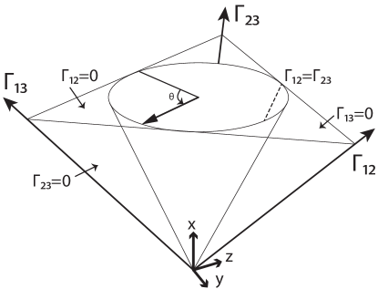
Figure 1: Convex cone of allowed dephasing rates for $N=3$ and real dephasing, i.e., $\Delta\omega_{23}=0$. The axes are $x=(\Gamma_{12}+\Gamma_{23}+\Gamma_{13})/\sqrt{3}$, $y=\tfrac{1}{\sqrt{2}}(\Gamma_{13}-\Gamma_{23})$ and $z=\sqrt{\tfrac{2}{3}}\left(\Gamma_{12}-\tfrac{1}{\sqrt{2}}(\Gamma_{13}+\Gamma_{23})\right)$ and the constraint equation becomes $x^{2}/2\geq y^{2}+z^{2}$, which defines a circular cone in the positive octant of in the parameter space of $\{\Gamma_{12},\Gamma_{23},\Gamma_{13}\}$, tangential to the $\Gamma_{12}\Gamma_{23}$, $\Gamma_{23}\Gamma_{13}$, and $\Gamma_{13}\Gamma_{12}$ planes.

Speed Limits for Entanglement Decay

The constraints for the decoherence rates and frequency shifts have important implications for a wide range of physical, chemical and biological systems where phase relaxation is a dominant process. A consequence is the imposition of relative speed limits on the rates at which coherences can decay, especially in multi-partite systems where entanglement decay is strictly bounded above by the single qubit dephasing rates. Dephasing can be spatially correlated, the Markovian condition only constrains the temporal correlations in the noise. In general, the dephasing rates can be of a non-local form.

Let us start with two qubits where we label the basis states by $|1\rangle=|00\rangle$, $|2\rangle=|01\rangle$, $|3\rangle=|10\rangle$ and $|4\rangle=|11\rangle$. Assuming that both qubits have the same local dephasing rate, i.e. $\Gamma=\Gamma_{12}=\Gamma_{13}=\Gamma_{24}=\Gamma_{34}$, then the allowed decoherence rates for the non-local coherences $\Gamma_{14}$ and $\Gamma_{23}$ are determined by $\Gamma$. The first non-trivial constraint $(a_{2}^{(3)})^{2}\geq 0$ gives $0\leq\Gamma_{23}\leq 4\Gamma$. The second constraint $(a_{3}^{(4)})^{2}\geq 0$ leads to $\Gamma_{23}+\Gamma_{14}\leq 4\Gamma$ . Thus, to ensure complete positivity of the evolution, the non-local coherences $\rho_{23}$ and $\rho_{14}$ can decay at most four times as fast as the local coherences, and the sum of the non-local decay rates can be no more than $4\Gamma$. If they are equal $\Gamma_{23}=\Gamma_{14}=\Gamma_{e}$ we obtain $\Gamma_{e}\leq 2\Gamma$, and Fig. 2 demonstrates that violation of the bound leads to violations of positivity, i.e., non-physical states.

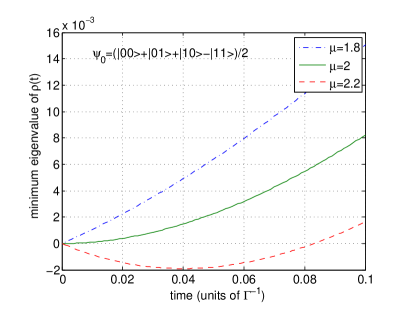
Figure 2: Constraint violation leads to non-physical states. A plot of the minimum eigenvalue of $\rho(t)$ starting with $\rho_{0}=|\Psi_{0}\rangle\langle\Psi_{0}|$ subject to pure dephasing $(H=0)$ with $\Gamma_{23}=\Gamma_{14}=\mu\Gamma$ for different values of $\mu$ shows the emergence of negative eigenvalues for $\mu>2$.

The limits to non-local coherence decay relate to the entanglement between qubits. Starting with the maximally entangled Bell state $|\Psi_{0}\rangle=\tfrac{1}{\sqrt{2}}(|00\rangle+|11\rangle)$, the state evolving under pure dephasing

$$\rho_{\Psi_{0}}(t)=\frac{1}{2}\begin{pmatrix}1&0&0&e^{-t\Gamma_{14}}\\ 0&0&0&0\\ 0&0&0&0\\ e^{-t\Gamma_{14}}&0&0&1\end{pmatrix}$$

has concurrence $C(t)=e^{-t\Gamma_{14}}$ Wootters2001 , thus $\Gamma_{14}+\Gamma_{23}\leq 4\Gamma$ implies that the concurrence cannot decay faster than four times the local decoherence rate $\Gamma$. Here, the decay of non-local coherences is not lower bounded, i.e. non-local coherences can survive indefinitely even for finite local decay rates and in this case the entanglement is preserved if $\Gamma_{14}=0$, i.e. there is no sudden death of entanglement YuEberly2004 .

Alternatively, starting with the maximally entangled two-qubit cluster state $|\Psi_{CS}\rangle=\frac{1}{2}(|00\rangle+|01\rangle+|10\rangle-|11\rangle)$, we obtain

$$\rho_{CS}(t)=\frac{1}{4}\begin{pmatrix}1&e^{-\Gamma t}&e^{-\Gamma t}&-e^{\Gamma_{14}t}\\ e^{-\Gamma t}&1&e^{-\Gamma_{23}t}&-e^{-\Gamma t}\\ e^{-\Gamma t}&e^{-\Gamma_{23}t}&1&-e^{-\Gamma t}\\ -e^{-\Gamma_{14}t}&-e^{-\Gamma t}&-e^{-\Gamma t}&-1\end{pmatrix}.$$

In this case the entanglement can decay even if both non-local dephasing rates vanish, $\Gamma_{14}=\Gamma_{23}=0$, in which case the concurrence satisfies $2C_{1}(t)=|e^{-\Gamma t}+1|-|e^{-\Gamma t}-1|$, which tends to zero as $t\to\infty$. If one of the two non-local concurrences is $4\Gamma$ and the other is $0$, e.g., $\Gamma_{14}=4\Gamma$, $\Gamma_{23}=0$, the concurrence similarly decays asympotically but faster. When the non-local coherences decay at the same rate $\Gamma_{14}=\Gamma_{23}=2\Gamma$ we have $C_{2}(t)=\max\{0,\tfrac{1}{2}(2e^{-\Gamma t}+e^{-2\Gamma t}-1)\}$, and the concurrence vanishes when $2e^{-\Gamma t}+e^{-2\Gamma t}-1=0$, i.e. $t_{*}=-\Gamma^{-1}\log(\sqrt{2}-1)\approx 0.383\Gamma^{-1}$, i.e., we observe sudden death of entanglement rather than asymptotic decay.

We can extend this to $n$-qubit systems. Given $n$ qubits with the same local dephasing rate $\Gamma$, we can simply apply the results above to any subsystem consisting of two qubits, i.e., the entanglement between any two qubits in the system cannot decay faster than $2\Gamma$. For larger systems there are more constraints so in practice the rate of entanglement decay between any two qubits would be even more restricted. For example for a three-qubit system with have $N=2^{3}=8$. Assuming the local dephasing rate for each qubit is $\Gamma$, and the dephasing rate involving two- and three-qubit transition terms are $\mu_{1}\Gamma$ and $\mu_{2}\Gamma$, respectively, there are 8 constraints restricting the allowed values for $\mu_{1}$ and $\mu_{2}$. From the constraints for the two-qubit system we know that $0\leq\mu_{1}\leq 2$, but Fig. 3 shows that the set of $(\mu_{1},\mu_{2})$ that satisfy all the constraints is much smaller. Each additional constraint reduces the set of allowed dephasing rates.

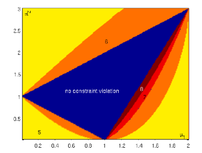
Figure 3: Constraint violation map for three qubits with local dephasing rates $\Gamma$, two-qubit dephasing rates $\mu_{1}\Gamma$, and three-qubit dephasing rates $\mu_{2}\Gamma$. For $0\leq\mu_{1}\leq 2$ the first four of the eight constraints are satisfied but additional constraints may be violated, e.g. in the yellow region, constraint 5 is violated. Each subsequent constraint further restricts the set of allowed rates.

Discussion

The underlying basis for the dephasing constraints is correlations between noise acting on different energy levels of the system. The canonical dephasing operators reflect underlying physical processes with different correlation properties. For example, a canonical dephasing operator with a single non-zero element can be interpreted as the result of the fluctuation of a single energy level. Multiple non-zero diagonal entries correspond to correlated perturbation of more than one level. These fluctuations can be correlated across levels even for Markovian dynamics where the noise statistics are temporally uncorrelated.

An example of where noise correlation can occur is magnetic field fluctuations acting on a spin-1 particle where the coupling is of the form $B_{Z}S_{Z}$. This leads to anti-phase perturbations of the $S_{Z}=\pm 1$ levels and the canonical operator in the basis $\{|0\rangle,|1\rangle,|-1\rangle\}$ is $\propto\operatorname{diag}(0,1,-1)$. If the coupling was instead of the form $B_{Z}S_{Z}^{2}$, then the canonical operator would be $\propto\operatorname{diag}(0,1,1)$.

Dephasing not only can lead to exponential damping of the coherences but also can produce shifts in their frequencies. Not all of these frequency perturbations can be accommodated by modifying the system Hamiltonian in general, the residual shifts are intrisic to the decoherence processes. Whilst pure damping can be generated by phase diffusion due to random drift of the energy levels (Wiener-Levy process) Wodkiewicz1979 , the frequency shifts can be caused by phase kicks, or discrete random phase jumps with a poissonian arrival time, though this also produces additional damping Herzog1995 . Phase kicks occur, for example, by collisional processes in gases, whereas phase diffusion can be generated by white noise acting on the energy levels.

It is possible to derive dephasing constraints from physical models of the noise directly, though deriving the general multi-level constraints is considerably more difficult than the methods shown here. However, once the observed dephasing rates have beeen decomposed into their corresponding canonical set of dephasing operators, we can assign physical mechanisms by which they occur, and hence perform system diagnostis or analysis. The ability to identify sources of dephasing will be vital in producing coherent quantum devices and improving their performance.

In the context of multi-partite systems, the constraints we have derived have implications for the preservation of non-local correlations. As the number of parties increases, the decay of the non-local coherences becomes constrained even more by the local dephasing rates. This reflects the general robustness of the non-local correlations in multi-partite systems MultiPartCorrelationRobustness . Conversely, there are suggestions that dephasing can play a positive role in biological processes Plenio2008 ; Plenio2008 . Dephasing has been mooted to enhance the transport of energy networks such as photosynthetic harvesting complexes. In such systems, measurement and analysis of the dephasing may illuminate these processes and lead to better energy collection devices.

Methods

Canonical dephasing operators. We start with the Lindblad master equation (LME) for Markovian open quantum system evolution

$$\dot{\rho}(t)=-i(H\rho(t)-\rho(t)H)+\mathfrak{L}_{D}(\rho(t)),$$ (6)

where $\rho(t)$ is the density operator describing the system state (defined on the system Hilbert space $\mathcal{H}_{s}$), $H$ is an effective Hamiltonian $H$ and the superoperator $\mathfrak{L}_{D}(\rho)$ takes the form $\mathfrak{L}_{D}(\rho)=\sum_{k}\mathcal{D}[V_{k}]\rho$ with Lindblad1976 ; GKS1976

$$\mathcal{D}[V_{k}]\rho=V_{k}\rho V_{k}^{\dagger}-\tfrac{1}{2}(V_{k}^{\dagger}V_{k}\rho+\rho V_{k}^{\dagger}V_{k}).$$ (7)

for operators $V_{k}$ on $\mathcal{H}_{S}$.

The operators $(H,V_{k})$ define a pure dephasing process with respect to the basis $\mathfrak{B}=\{|n\rangle\}_{n=1}^{N}$ if and only if $H$ and all $V_{k}$ are simultaneously diagonal with respect to $\mathfrak{B}$, i.e., we have

$$H =\sum_{n}\lambda_{n}\Pi_{n}=\operatorname{diag}(\lambda_{n}),\quad\lambda_{n}\in\mathbb{R}$$ (8a)

$$V_{k} =\sum_{n}\gamma_{nk}\Pi_{n}=\operatorname{diag}(\gamma_{nk}).$$ (8b)

This is easy to see since by definition of a pure dephasing process the populations of the basis states remain constant, and thus each basis state $|n\rangle$ is a steady state of the system. This is possible only if the subspace spanned by each basis state $|n\rangle$ is $V_{k}$-invariant for all $V_{k}$ SW2010 . This shows that all $V_{k}$ must be diagonal in the chosen basis. Since $\Pi_{n}$ is diagonal and diagonal operators commute we have $\mathcal{D}[V_{k}](\Pi_{n})=0$ for all $n$ and all $k$. As $|n\rangle$ is a steady state, i.e., $\dot{\Pi}_{n}(t)=0$, it also follows that $-iH\Pi_{n}+i\Pi_{n}H=0$ for all $n$. Inserting this into the general form of the LME (6) gives the explicit equation

$$\dot{\rho}_{mn}(t)=-\left(i\omega_{mn}+\Gamma_{mn}\right)\rho_{mn}(t),$$ (9)

for the evolution of the matrix elements $\rho_{mn}=\langle m|\rho|n\rangle$ of the density operator, or in integral form (2) with frequencies $\omega_{mn}=\lambda_{m}-\lambda_{n}+\Delta\omega_{mn}$ and dephasing induced frequency shifts and decoherence rates given by (3).

Any set of diagonal Lindblad operators $\{V_{k}\}$ generates pure dephasing dynamics but the set of Lindblad operators $\{V_{k}\}$ generating a certain dynamical evolution is not unique. In particular, we have unitary invariance, i.e., given any set of Lindblad operators $\{V_{k}\}$, the set of operators $\{W_{j}\}$ defined by

$$W_{j}=\sum_{k}u_{jk}V_{k},$$ (10)

where $u_{jk}$ are elements of a unitary matrix, generates the same dynamics as $\sum_{k}\mathcal{D}[W_{k}]\rho=\sum_{k}\mathcal{D}[V_{k}]\rho$. Furthermore adding multiples of the identity, $V_{k}\to V_{k}+\alpha\mathbb{I}$, to a Lindblad operator $V_{k}$ only changes the effective Hamiltonian

$$\mathcal{D}[V_{k}+\alpha\mathbb{I}]\rho=\tfrac{1}{2}[\alpha V_{k}^{\dagger}-\alpha^{*}V_{k},\rho(t)]+\mathcal{D}[V_{k}]\rho,$$ (11)

and thus the dynamics is unchanged if we replace $V_{k}$ by $V_{k}+\alpha\mathbb{I}$ and $H$ by $H+\tfrac{i}{2}(\alpha V_{k}^{\dagger}-\alpha^{*}V_{k})$.

The invariance of the dephasing dynamics under the two “gauge transformations” (10) and (11) allows us to transform any set of dephasing operators $\{V_{\ell}\}$ into an equivalent set of dephasing operators in canonical form defined in Eq. (1), which yield the same observable dephasing rates $\{\Gamma_{mn}\}$ and dephasing shifts $\{\Delta\omega_{mn}\}$, using Algorithm 1. The process is constructive and, using $a_{nk}$ intead of $a_{n}^{(k)}$, the key steps can be described as follows:

(1) Using (11) we ensure that $a_{1k}=0$ for all $V_{k}$, modifying the Hamiltonian by

$$\Delta H=\frac{i}{2}\sum_{k}a_{1k}V_{k}^{\dagger}-a_{1k}^{*}V_{k}$$ (12)

as necessary.

(2) We replace the Lindblad operators $V_{1}=\operatorname{diag}(0,a_{21},a_{31},\ldots)$ and $V_{2}=\operatorname{diag}(0,a_{22},b_{32},\ldots)$ with $a_{21}=r_{21}e^{i\phi_{21}}$ and $a_{22}=r_{22}e^{i\phi_{22}}$ by $\{W_{1},W_{2}\}$ with

$$W_{1} =u_{11}V_{1}+u_{12}V_{2}=\operatorname{diag}(0,c,\ldots)$$ (13a)

$$W_{2} =u_{21}V_{1}+u_{22}V_{2}=\operatorname{diag}(0,0,*,\ldots)$$ (13b)

with the unitary coefficient matrix

$$u=\frac{1}{c}\begin{pmatrix}r_{21}e^{i\phi_{22}}&r_{22}e^{i\phi_{21}}\\ r_{22}e^{-i\phi_{21}}&-r_{21}e^{-i\phi_{22}}\end{pmatrix}$$ (14)

and $c=\sqrt{r_{21}^{2}+r_{22}^{2}}$, which is dynamically equivalent to $\{V_{1},V_{2}\}$ due to (10).

This result allows us to reduce an arbitrary number of parameters, specified by the non-zero elements of a general set $\{V_{k}\}$ of dephasing operators to $N(N-1)/2$ parameters in the canonical form. Note that the number of free parameters matches the number of dephasing rates $\Gamma_{mn}$ for an $N$-level system. The procedure will work, i.e., to produce a set of canonical dephasing operators that reproduce the observed dephasing rates and shifts, provided that these satisfy the positivity constraints. Furthermore, if the observed dephasing rates and shifts lead to constraint violations these will be detected and flagged, and this information can be used to further investigate if the violations can be explained in terms of uncertainty in the observed data, e.g., due to measurement errors, or if they are indicative of processes that would invalidate the Markovian dephasing assumption.

We note that if one has the usual Kossakowski form of Markovian evolution GKS1976 , we can “diagonalise” the sets of operators to arrive at a Lindblad form Lindblad1976 where the decoherence operators are orthogonal and traceless. However, this standard form is not convenient for inversion, nor does it give much physical insight into the possible processes leading to dephasing. The canonical form Eq. 1 decomposes the dephasing into operators representing correlated level perturbations of orders 1 to N-1.

$V$ $\leftarrow$ CanonicDephasing ($W$)
Calculate Canonical Dephasing Operators
In:	$W$	Matrix $(N\times K)$, $k$th column equals diagonal elements of Lindblad operator $V_{k}$
Out:	$V$	Lower triagonal matrix, columns equals diagonal elements of canonical $V_{k}$
1 $R$ $\leftarrow$ Number of rows of $W$ 2 $C$ $\leftarrow$ Number of columns of $W$ 3 $V$ $\leftarrow$ $W-$ones$(R,1)*W[1,:]$ 4 $k$ $\leftarrow$ $1$  // Running column index 5 for $r$ $\leftarrow$ $2,\ldots,N$ 6 $i_{1}$ $\leftarrow$ Index 1st nonzero entry of $V[r,k:C]$ 7 $i_{1}$ $\leftarrow$ $i_{1}+k-1$  // shift index 8 while more than one element of $V[r,k:C]$ non-zero 9 $i_{2}$ $\leftarrow$ Index 2nd nonzero entry of $V[r,k:C]$ 10 $i_{2}$ $\leftarrow$ $i_{2}+k-1$  // shift index 11 $r_{1}$ $\leftarrow$ $|V[r,i_{1}]|$, $r_{2}$ $\leftarrow$ $|V[r,i_{2}]|$ 12 $\phi_{1}$ $\leftarrow$ Phase$(V[r,i_{1}])$, $\phi_{2}$ $\leftarrow$ Phase$(V[r,i_{2}])$ 13 $n_{c}$ $\leftarrow$ $\sqrt{r_{1}^{2}+r_{2}^{2}}$ 14 $V[:,i_{1}]$ $\leftarrow$ $(r_{1}e^{+i\phi_{2}}V[:,i_{1}]+r_{2}e^{+i\phi_{1}}V[:,i_{2}])/n_{c}$ 15 $V[:,i_{2}]$ $\leftarrow$ $(r_{2}e^{-i\phi_{1}}V[:,i_{1}]-r_{1}e^{-i\phi_{2}}V[:,i_{2}])/n_{c}$ 16 if $V[r,k:C]$ has non-zero entries 17 $k_{0}$ $\leftarrow$ Index of 1st non-zero entry 18 $k_{0}$ $\leftarrow$ $k_{0}+k-1$ 19 $V$ $\leftarrow$ Swap columns $k$ and $k_{0}$ of $V$ 20 $k$ $\leftarrow$ $k+1$ 21 $V$ $\leftarrow$ Remove $0$ columns of $V$, apply phase corrections

Algorithm 1: Canonical Dephasing Operators

I Acknowledgements

DKLO acknowledges support from the Quantum Information Scotland network (QUISCO). SGS acknowledges funding from EPSRC ARF Grant EP/D07192X/1 and Hitachi.

References

- (1) Schrödinger, E. (1936), Proc. Cam. Phil. Soc. 31, 555 (1936)
- (2) J.S. Bell, Physics 1, 195-200 (1964)
- (3) D. Deutsch, Proc. R. Soc. Lond. A 400, 97 (1985)
- (4) C. H. Bennett, G. Brassard, C. Crépeau, R. Jozsa, A. Peres, W. K. Wootters, Phys. Rev. Lett. 70, 1895-1899 (1993)
- (5) A. K. Ekert, Phys. Rev. Lett. 67, 661 (1991)
- (6) Caves, C. M., Phys. Rev. D 23, 1693-1708 (1981).
- (7) G. S. Engel et al., Nature 446, 782 (2007)
- (8) W. H. Zurek, Phys, Rev, D, 24, 1516 (1981)
- (9) G. M. Palma, K.-A. Suominen and A. K. Ekert, Proc. Roy. Soc. London Ser. A 452, 567 (1996)
- (10) S. G. Schirmer and A. I. Solomon, Phys. Rev. A 70, 022107 (2004)
- (11) P. R. Berman and R. C. O’Connell, Phys. Rev. A 71, 022501 (2005)
- (12) K. Kraus, Ann. Phys. 64, 311 (1971)
- (13) G. Lindblad, Commun. Math. Phys. 48, 119 (1976)
- (14) W. Gorini, A. Kossakowski and E. C. G. Sudarshan, J. Math. Phys. 17, 821 (1976)
- (15) W. K. Wootters, Quant. Inf. and Comp. 1, 27 (2001).
- (16) T. Yu and J. H. Eberly, Phys. Rev. B 66, 193306 (2002)
- (17) T. Yu and J. H. Eberly, Phys. Rev. Lett. 93, 140404, (2004)
- (18) K. Wodkiewicz, Phys. Rev. A 19, 1686 (1979).
- (19) U. Herzog, Phys. Rev. A 52, 602 (1995)
- (20) S. G. Schirmer and Xiaoting Wang, Phys. Rev. A 81, 062306 (2010), Eq. (11)
- (21) Z-X. Man, Y-J. Xia and N. V. An, Phys. Rev A 78, 064301 (2008); M. Sarovar, A. Ishizaki, G. R. Fleming, K. B. Whaley, Nature Physics 6, 462 (2010); C. Simon and J. Kempe, Phys. Rev. A 65, 052327 (2002)
- (22) M.B. Plenio, S.F. Huelga, New J. Phys. 10, 113019 (2008)
- (23) P. Rebentrost, M. Mohseni, I. Kassal, S. Lloyd, A. Aspuru-Guzik, New J. Phys. 11, 033003 (2009)