A probability-conserving cross-section biasing mechanism for variance reduction in Monte Carlo particle transport calculations

Abstract

In Monte Carlo particle transport codes, it is often important to adjust reaction cross sections to reduce the variance of calculations of relatively rare events, in a technique known as non-analogous Monte Carlo. We present the theory and sample code for a Geant4 process which allows the cross section of a G4VDiscreteProcess to be scaled, while adjusting track weights so as to mitigate the effects of altered primary beam depletion induced by the cross section change. This makes it possible to increase the cross section of nuclear reactions by factors exceeding $10^{4}$ (in appropriate cases), without distorting the results of energy deposition calculations or coincidence rates. The procedure is also valid for bias factors less than unity, which is useful, for example, in problems that involve computation of particle penetration deep into a target, such as occurs in atmospheric showers or in shielding.

1 Background

In any Monte-Carlo particle transport calculation, the quality of the computed result is limited by the statistical uncertainty in the counting of the random events that are modeled. Often it is interesting to compute the probability of very rare events, since these may have particularly large significance in certain applications. A typical example of relevance to the semiconductor community is single event effects (SEEs) created by the breakup of a heavy nucleus by an incoming cosmic ray. Such events may be very rare, but because they can cause a single incoming particle to create multiple outgoing particles, often with very high linear energy transfer (LET), they can foil SEE mitigation techniques which rely on an assumption that only one device in a region can be upset by an individual event [1, 2, 3]. Rare events can also be generated in a converse situation, in which the very strong absorption of particles makes it difficult to look at the types of events that are due to particles that have penetrated very deeply into the material, as would be the case for events due to particles that have penetrated shielding.

To improve the statistical variance in such calculations, it is common to modify the cross section for potentially interesting processes, and to appropriately weight the resulting calculation to compensate for this modification. In the MRED code at Vanderbilt [1], we have been using such a technique for many years, by incorporating conventional Geant4 hadronic processes in a cross-section biasing wrapper. The wrapped process increases cross sections by a biasing factor $b$, and scales the weight of tracks in which a biased process occurs by a factor $1/b$. To first order, this is a very effective technique, but it has limits as to how much bias can be applied. Often, in small geometries, bias factors of a few hundred can be used, resulting in roughly equal decreases in the computational effort required to quantify effects involving nuclear reactions. Factors of a this order are clearly significant, and can be critically important considering the practical costs of computing.

There are two limiting factors which control how much one can upwardly bias the cross section of a process in a Monte-Carlo calculation framework such as Geant4 [4]. The first one, incoming beam depletion, is addressed by this paper. If beam depletion is ignored, there is a distortion of computed effects that is dependent upon the amount of material an incoming particle has crossed before it interacts. The second is innate to all types of Monte-Carlo codes; if one enhances the probability of one class of event, it is at the cost of reducing the statistics for some other class. Depending on the purpose of a given calculation, one may be forced to limit the bias factor so that events in which no reaction in the biased category occur still get some significant sampling weight.

The problem of incoming particle depletion is, in brief, as follows. As a particle traverses a material, it has a probability of being deflected or destroyed by a collision with an atom in the target. For typical nuclear cross sections, this results in an attenuation of the incoming particle flux with a length scale of the order of a few centimeters. This part is purely physical. However, if one enhances the cross section for interaction by a factor $b$, the attenuation length is unphysically reduced by the same factor. Conversely, reducing the cross section allows a simulated particle to penetrate too deeply, and must be compensated by reducing its statistical weight. This results in the under-sampling or oversampling of events as one progresses into the target. We present, in the next section, a quantitative mechanism to account for these effects.

The approach we present stands in contrast to methods known as particle splitting techniques [5, 6]. In those techniques, one takes each simulated particle, and when an interaction occurs, splits the history into two branches, one that contains the interaction products, and the other that carries away the original particle with a modified statistical weight and allows it to further interact. Instead of dealing with the weight adjustment discretely, as in particle splitting, we correct for the effects of the cross section bias in an average manner along the particle path. This greatly simplifies the book keeping relative to particle splitting, and allows the benefits of biasing to be incorporated into conventional Monte-Carlo codes with almost no modification to the structure of the code itself.

2 Basic depletion argument

As a particle propagates through a material, the probability $P(x)$ of it reaching a point $x$ is set by the solution of:

$$\frac{dP(x)}{P(x)}=-\rho(x)\,\sigma(x,\,E(x))\,dx$$ (1)

where $\rho$ is the material density in scatterers/volume, $\sigma$ is the cross section for an interaction, and $x$ is the distance travelled along the particle path, in the absence of any biasing of the probabilities. This equation only takes account of binary interactions of the incoming particle with the target material, and ignores spontaneous decay of the particle. The treatment presented needs to be modified if particle decay in flight is included; we do not treat this case here. If we bias $\sigma$ by a factor $b$, then the probability is modified:

$$\frac{dP_{b}(x)}{P_{b}(x)}=-b\rho(x)\,\sigma(x,\,E(x))\,dx$$ (2)

which, noting that

$$\frac{d(f/g)}{f/g}=\frac{df}{f}-\frac{dg}{g}$$ (3)

results in an extra depletion of the probability of it penetrating to $x$ of

$$\frac{d\left(P_{b}(x)/P(x)\right)}{P_{b}(x)/P(x)}=-(b-1)\rho(x)\,\sigma(x,\,E(x))\,dx$$ (4)

If one therefore gradually adjusts the statistical weight $W$ of a particle according to:

$$\frac{dW(x)}{W(x)}=(b-1)\rho(x)\,\sigma(x,\,E(x))\,dx$$ (5)

then, the weighted probability $P_{b}(x)W(x)$ will be equal to the original probability $P(x)$. This effectively conserves particle flux, albeit by carrying a smaller number of more heavily weighted particles (in the case of $b>1)$.

In typical simulations, one takes discrete steps over which the parameters are held constant. At the end of such a simulation step, where $\rho$ and $\sigma$ are taken to be constant,

$$\frac{\Delta W(x)}{W(x)}=(b-1)\rho(x)\,\sigma(x,\,E(x))\,\Delta x\\ \equiv(b-1)\times\Delta\lambda$$ (6)

where $\Delta\lambda$ is the number of physical interaction lengths traversed in this step. The solution to this is:

$$W(x)=W(x-\Delta x)\times\exp\left((b-1)\times\Delta\lambda\right)$$ (7)

The effect of applying this correction is that the weight of particles is adjusted in an average sense. Instead of tracking each individual step of each particle, and adjusting the weight and splitting particle histories so that probability is exactly conserved depending upon the events that befall a particular particle, this approach corrects the weight so that the average effect of this correction compensates the average error due to the adjustment of the strength of an interaction. Since, from equation 4, we know the exact value of the correction, this approach is statistically exact. That is all that is needed for a calculation to produce an unbiased result using a statistical method such as Monte Carlo integration.

As will be seen graphically in the examples below, the selection of the bias parameter for a given problem is not too critical. If the bias parameter is far too small (in the case of thin target problems, where it is greater than unity), many of the particles penetrate the target without interacting, resulting in lower computational efficiency. If the bias parameter is far too large (only a small fraction of the particles not interacting), the statistical quality of points deep in the target will be degraded due to beam depletion, although the computed mean value will still be unchanged. The converse is true for thick-target situations, where one is reducing the cross section to permit penetration, but the outcome is the same. As a result, it is generally very efficient to choose a bias such that roughly half of the particles are absorbed; this achieves a balance between the number of particles that interact and the statistical significance for particles that have penetrated far into the target.

3 Procedure for applying the bias correction

In a typical Monte-Carlo particle transport code, particles interact with their environment through two classes of processes:

1. Discrete processes, which represent point-like interactions of the particle with another particle in its proximity, and,

2. Continuous processes, which represent smooth drag-like terms which occur along the entire length of each step in a particle’s trajectory.

Also, it is assumed a particle carries along with it a statistical weight $w$ that can be modified as it propagates, and that can be passed along as a starting weight to any daughter particles created.

The method we describe is specifically applicable to the discrete processes. The procedure for transporting a particle along one step of a trajectory is roughly as follows:

1. Start with a particle at position $\vec{x_{0}}$ with energy $E_{0}$

2. Compute a transport length $L_{\mathrm{trans}}$ for the next step the particle will take, based on the summed strength of the interaction processes computed at position $\vec{x}_{0}$ and energy $E_{0}$.

3. Randomly select which of multiple discrete interaction processes will be invoked at the end of the step, based on the individual strengths of the applicable processes.

4. Move particle forward a distance $L_{\mathrm{trans}}$ along its current momentum direction.

5. Compute the effects which all applicable continuous interactions would have had on the particle, and update its parameters based on those effects.

6. Multiply the particle’s statistical weight by

   $$\prod_{i=1}^{n}\exp\left(\left(b_{i}-1\right)\times L_{\mathrm{trans}}\times N\times\sigma_{i}\right)$$ (8)

   where $i$ indexes over the active discrete processes, $b_{i}$ and $\sigma_{i}$ are the bias in effect and the cross section for the $i^{th}$ process at this step, and $N$ is the material particle density along the step such that $L_{\mathrm{trans}}N\sigma=\Delta\lambda$ as defined in equation 7.

7. Multiply the particle’s statistical weight by $1/b_{j}$ where the index $j$ is that associated with the process chosen in step 3.

8. Invoke the discrete interaction selected in step 3, and update the particle’s parameters. Create daughter particles with the current statistical weight of the parent.

4 Management of statistical weights

At the end of tracking of all the particles that are created during a simulation event, one typically accumulates the information about how energy was deposited by those particles. We define the following quantities, assuming the particle indexed by $k$ in the event starts out with weight $w_{k,0}$.

The statistical weight of the $k^{th}$ particle at the end of the $n^{th}$ step along its trajectory is:

$$w_{k,n}=w_{k,0}\prod_{l=1}^{N{}_{\mathrm{b}\,k,n}}\frac{1}{B_{k,l}}\prod_{m=1}^{n}\prod_{i=1}^{N{}_{\mathrm{p}\,k}}\exp\left(\left(b_{k,m,i}-1\right)\times\Delta\lambda_{k,m,i}\right)$$ (9)

where the terms are as defined in eq. 7 except that $b_{k,m,i}$ and $\lambda_{k,m,i}$ refer specifically to the bias and scaled interaction length that were applicable to the $i^{th}$ process along the $m^{th}$ step, $N{}_{\mathrm{p}\,k}$ is the number of processes for the $k^{th}$ particle, $B_{k,l}$ is the $l^{th}$ discrete bias applied to the $k^{th}$ particle, and $N{}_{\mathrm{b}\,k,n}$ is the number of discrete interactions with a bias factor different than $1$ that have been applied to the $k^{th}$ particle prior to and including the $n^{th}$ step. This is just the accumulated result of eq. 8 along all the steps, including multiple processes creating biases. If a particle interacts at step $n$ and produces daughters, the daughter tracks are created with a weight $w_{k,n}$ of the parent particle $k$.

Also, define a weight for an entire event,

$$W_{\mathrm{e}}=w_{0}\,\prod_{l=1}^{N_{\mathrm{int}}}\frac{1}{B_{l}}\prod_{k=1}^{N_{\mathrm{part}}}\prod_{m=1}^{N_{\mathrm{steps}\,k}}\prod_{i=1}^{N_{\mathrm{p}\,m}}\exp\left(\left(b_{k,m,i}-1\right)\times\Delta\lambda_{k,m,i}\right)$$ (10)

where, in this case, it is assumed the event started with a statistical weight $w_{0}$, $N_{\mathrm{int}}$ discrete interactions occurred in the course of the event, each biased by a factor $B_{l}$, $N_{\mathrm{part}}$ is the number of particles in the entire event, $N_{\mathrm{steps}\,k}$ is the number of steps for the $k^{th}$ particle, and the inner product runs over all segments of all tracks in the event, with $b_{k,m,i}$ and $\lambda_{k,m,i}$ as in eq. 9. This accumulates all of the weight modifications from the event. Note that the book-keeping here creates a result that is not simply the products of the weights of all the particles in the event at the end of their trajectory. Since an interaction may produce multiple daughters, the product of all the final weights contains replicates of the bias that is introduced by an interaction. Eq. 10 counts each bias exactly once.

It is necessary to consider the meaning of the statistical weights that can be computed by this process. This is a somewhat complex issue, because, in different use cases, it may be necessary to treat the tracks in the event as individual entities, each with a distinct statistical weight, or to treat the entirety of the event as a single ensemble with one global weight. The difference between these two approaches depends on assumptions of correlated or uncorrelated statistical probabilities. The two cases just described are the limiting cases, and result in easy-to-interpret statistics. More complex cases could be considered, in which one wishes to calculate the joint probability of two arbitrary tracks in an event. In this case, it is necessary to look at their parent lineage, and compute the statistics with the knowledge that when they share a vertex, the statistical weight change resulting from that shared vertex is fully correlated, while changes which occur after they no longer share a vertex are uncorrelated. We do not consider this in the discussion below, because it is not relevant to the most common use cases.

The weight obtained from eq. 10 is the effective statistical weight for all the correlated components which have happened in an event. If the event is to be treated as a whole, single object, as in non-Boltzmann tallies such as energy depositions in sensitive detectors being entered into a histogram as pulse heights, or as contributions to a coincidence rate, all tracks of the event should be treated as having this single weight, and the individual weights on the tracks should be ignored. In the typical format of a call to a histogramming tool such as AIDA [7, 8], one would execute a call such as fill() to add an event of amplitude $E_{\mathrm{dep}}$ with weight $W_{\mathrm{e}}$ to accumulate the result from a sensitive detector at the end of an event.

On the other hand, if one is computing total dose (for example), where each track and step in the event is treated independently and one is computing an integral across many events, the weights which are left attached to the individual tracks are the appropriate weights to use. Each particle in the event has a specific probability of being created by its parent, and this is properly accounted for by eq. 9. The appropriate mechanism for adding energy into a calorimeter is to add $E_{\mathrm{dep}\,k,n}\times w_{k,n}$, where $w_{k,n}$ is as defined in eq. 9 and $E_{\mathrm{dep}\,k,n}$ is the energy deposited by the $k^{th}$ particle during the $n^{th}$ step.

5 Specific Implementation in Geant4

In this section, we describe the details of the implementation of this process in Geant4. The purpose is both for the benefit of Geant4 users, and also to present code which is an actual implementation of eqs. 8 and 10, since the code may be easier to interpret or reuse than the formulas themselves.

This code is written as a wrapper for G4VDiscreteProcess in Geant4 (for information on all Geant4 specific information, see [9]), and exposes itself as a G4VContinuousDiscreteProcess, so that it can provide an AlongStepDoit() method to carry out the bias adjustment described in equation 7. It shares the bias factor among all instances of the wrapper, so that one can adjust all particles with a single call, without having to keep a registry of copies of this process, and adjust every one when the bias is changed. As discussed in the shielding example in section 6, there might be use cases for which there would be benefit in biasing different processes by different amounts. This should be easily adapted to that case.

The mechanism for using this process is as follows. For each G4VDiscreteProcess to be biased, one creates an instance of the wrapper with the already-created process to be wrapped as the argument to the constructor. This can either be done when the wrapped processes are originally created (in the physics list construction), or afterwards. To do it afterwards requires scanning the process tables for all particles for candidates to be wrapped, and replacing the process table entries with newly instantiated copies of the wrapper. This allows one to use the built-in Geant4 standard physics lists, and then apply the wrappers as an independent step. The results shown in section 6 were created using biased processes in HadronPhysicsQGSP_BIC_HP for the inelastic physics, and unbiased G4UHadronElasticProcess attached to the G4NeutronHPorLElastic model for the elastic scattering.

To interface with the event-based weighting created by this process requires code in the G4UserEventAction class, with a call to ResetAccumulatedWeight() in the BeginOfEventAction(). This resets the accumulated event weight to unity. Then, in the EndOfEventAction() or in G4VSensitiveDetector EndOfEvent() processing, one calls GetAccumulatedWeight() to retrieve the appropriate statistical weight for the event, as defined by eq. 10.

On the other hand, if one is computing total dose (for example), the appropriate mechanism for adding energy into a calorimeter is to add deposited_energy$\times$track.GetTrackWeight() (where the weight at the $n^{th}$ step is as defined in eq. 9) for each hit on a sensitive detector during the ongoing processing of an event. If this approach is being used, there is no need (although no harm) to call ResetAccumulatedWeight().

6 Sample runs showing the effects of biasing

In this section, we present examples, based on a few archetypal models. In the first set of examples, the system we use as our exemplar of increased bias is a $1\,\mathrm{mm}$ film of lightly borated $\left(\mathrm{CH}_{2}\right)_{n}$ (essentially polyethylene or polypropylene). It is irradiated with a monoenergetic neutron beam, with an energy of $0.025\,\mathrm{eV}$. The boron concentration is $0.1\,\mathrm{wt.}\%$ in some cases, and $0.2\,\mathrm{wt.}\%$ in others (indicated in each example). This results in weak depletion of the incoming beam in reality. The alpha particle production yield is calculated in 10 bins throughout the thickness of the film. The second case, of strong actual attenuation in a shielding computation, is best carried out with a bias of less than unity. In the final example, we present a coincidence rate calculation in a small target typical of semiconductor problems, demonstrating the ability of this technique in non-Boltzmann problems.

Figure 1: Comparison of $\alpha$ particle yield vs. depth in a $0.1\,\mathrm{wt.}\%$ boron loaded $\left(\mathrm{CH}_{2}\right)_{n}$ film with $0.025\,\mathrm{eV}$ incident neutrons. The bias=1 curve required 100 times as many events ($10^{7}$), and 25 times the computer time, as the bias=100 curve, for approximately the same statistical quality. Points have in the upper group of curves have been slightly shifted horizontally to avoid overlaps. Curves in this figure and figures below labeled ’uncorr.’ are for runs with biased cross sections, but do not include the weight correction of eq. 7; they are included since they show the level of primary beam depletion, which is an important measure of the strength of the biasing.

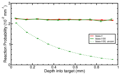
High-statistics accuracy demonstration

Figure 1 shows a yield comparison between a run with $10^{7}$ particles with a bias of 1, and $10^{5}$ particles with a bias of 100. Since the absorption is weak, most of the neutrons penetrate the target without interacting in the unbiased case. The computational time for the unbiased case is 25 times greater than that for the biased case, even though the number of particles run is 100 times greater. This discrepancy occurs because events that include an interaction take more time than those in which there is no interaction. Fig. 1 demonstrates three important points. First, the biased computation returns the same result as the unbiased one throughout the target thickness, even though there is significant depletion of the primary particles in the biased case. Second, because of increased computation associated with the larger number of reactions in the biased case, the efficiency of the computation increases sub-linearly with the bias, and would saturate when essentially all of the particles are interacting. Third, close examination of the plot shows that the uncertainty in the yield for the biased case increases with depth. This is because the increased depletion results in poorer statistics for particles that have traversed a larger distance. This effect also sets an upper limit on the bias that can be applied.

Figure 2: Comparison of $\alpha$ particle yield vs. depth in a $0.1\,\mathrm{wt.}\%$ boron loaded $\left(\mathrm{CH}_{2}\right)_{n}$ film with $0.025\,\mathrm{eV}$ incident neutrons. All of these data sets were run with the same number of events ($10^{5}$). Note that, in this example, the statistical uncertainties are fairly uniformly distributed for biases up to about 30. Points in the upper group of curves have been slightly shifted horizontally to avoid overlaps. See the fig. 1 caption for discussion of ’uncorr.’ curves.

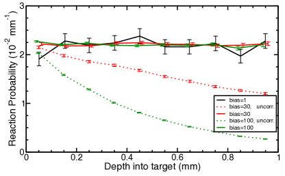
Moderately attenuated transport (bias well chosen)

Figure 2 shows a yield comparison made with $10^{5}$ particles in each run, using different bias factors, again on the $0.1\,\mathrm{wt.}\%$ target. The feature to observe in this result is that one can tune the distribution of errors by adjusting the bias, and that by turning the bias too high, the variance is increased for particles that are arriving in a region where the beam has been heavily depleted. In this case, although the result for a bias of 100 has smaller statistical errors at the entrance to the target than those for the bias of 30, it has larger errors at the exit. This behavior gives guidance about reasonable bias factors to use. In general, there is little to gain in a calculation if the bias is set so large that more than roughly half of the beam is depleted.

Figure 3: Comparison of $\alpha$ particle yield vs. depth in a $0.2\,\mathrm{wt.}\%$ boron loaded $\left(\mathrm{CH}_{2}\right)_{n}$ film with $0.025\,\mathrm{eV}$ incident neutrons. In this case, the higher boron concentration results in extreme beam depletion for the bias 100 run, and greatly increased statistical uncertainties of the yield for the points deepest into the target. Points in the upper group of curves have been slightly shifted horizontally to avoid overlaps. See the fig. 1 caption for discussion of ’uncorr.’ curves.

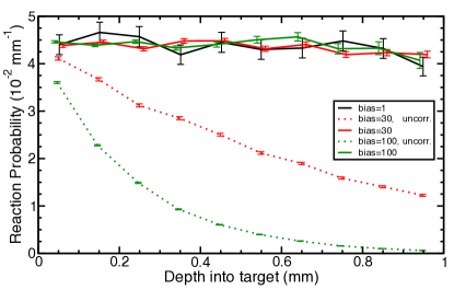
Strongly attenuated transport (bias too large)

Figure 3 shows the result of extreme depletion in the incoming beam, due to both strong absorption and high bias. In this case, the boron concentration in the target was raised to $0.2\,\mathrm{wt.}\%$. Since the transmission is exponential in the concentration, very little of the incoming beam is transmitted, and the statistical uncertainties for the highest bias are very large at the exit of the target. Although the result of the calculation still has the correct mean, its variance is very large.

Figure 4: Comparison of $\alpha$ particle yield vs. depth in a $5\,\mathrm{wt.}\%$ boron loaded $\left(\mathrm{CH}_{2}\right)_{n}$ film with a beam of $2\,\mathrm{eV}$ incident neutrons. Note that with bias less than unity, a shielding calculation can be carried out involving $10^{15}$ attenuation, using $10^{5}$ incident particles (red curve). See the fig. 1 caption for discussion of ’uncorr.’ curves.

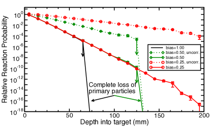
Shielding calculation (bias less than unity)

Figure 4 demonstrates the results of using the same biasing scheme, but with a $b$ value less than unity for both the inelastic and elastic processes. This demonstrates the important ability to use this biasing mechanism in cases in which the true primary beam depletion is so large that physics deep inside a target is poorly sampled. This case arises frequently in the computation of leakage of shielding systems, which can become very computationally expensive to carry out without variance reduction. This is equivalent to the “forced-flight” technique, such as is provided in the MCBEND code [10, 11], with the added flexibility that one can both calculate the attenuation of the primary particle flux, and the production of correctly-weighted secondaries.

Figure 5: Multilayer stack of materials, with two sensitive volumes (marked in dashed green lines). Coincidences were computed in this structure when it was irradiated from above with 6.4 GeV alpha particles. The heavy black arrows show a typical nuclear reaction event that could create a coincidence.

Coincidences (non-Boltzmann problem)

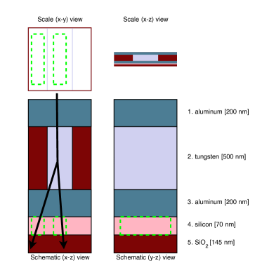
A final important case is a test of this weighting system in an explicitly non-Boltzmann transport problem. The archetype we use for this is a computation of a coincidence cross section for energy deposition in two volumes separated in space. In our test geometry, energy can be deposited in coincidence by nuclear reactions that include multiple particles in the outgoing channel. In figure 5 we show the target that was used to test the rate of coincidence generation, using the weighting in eq. 10. This target was exposed to $10^{5}$ $6.4\,\mathrm{GeV}$ alpha particles at normal incidence to the top, with a bias factor $b=10^{4}$, using the CREME Monte-Carlo tool [12]. A coincidence is determined to be an energy deposition of more than $10\,\mathrm{keV}$ in each of the sensitive volumes (shown as dotted green boxes in layer 4 of figure 5). For comparison, we also computed the coincidence cross section with unbiased statistics, running $10^{9}$ particles. The result was $(2.0\pm 0.2)\times 10^{-14}\,\mathrm{cm^{2}}$ for the biased case and $(2.2\pm 0.2)\times 10^{-14}\,\mathrm{cm^{2}}$ for the unbiased case. The computational time required for the biased case was 2 minutes; for the unbiased case, it was 27 hours.

7 Conclusion

This work presents a very simple mechanism for the adjustment of the effective strength of an interaction that can be described by a cross section, in a way that precisely preserves the mean transport characteristics, while allowing strong variance reduction. It allows one to efficiently calculate particle transport and scattering through solids in the extreme cases of either very weak or very strong scattering by the material, either of which can result in very large computational demands to achieve a low-variance result throughout the target material.

For targets that produce very little scattering of the incoming particles, the effective strength of the interaction can be increased, resulting in fewer particles that pass through the target un-scattered, and therefore less lost computation effort on particles that do not contribute to the final result. Conversely, for targets in which, in reality, most of the incoming particles would be absorbed before they penetrate to the depth of interest in the target, the computed interaction can be weakened to transport more particles to a greater depth into the target, and reduce the variance of results computed there.

In either case, the continuous adjustment of the weight of un-scattered particles combined with the specified computation of the total event weight assures that the computed transport properties remain unaffected by the introduction of the cross-section biasing factor. This holds true for both Boltzmann and non-Boltzmann type problems.

Appendix: Sample Geant4 implementation

The purpose for including an appendix in this paper with the source code for a complete Geant4 wrapper process that implements the above algorithm is twofold. First, the code is an alternative, iterative description of the deeply nested products in equations 9 and 10, and as such may prove more readable than the equations themselves, especially as they may be implemented in other codes. As documentation of the algorithm, it should not be too difficult to read around the Geant4-specific naming and structure to get to the functionality, which is almost entirely in the main code body. Second, the code should be able to be compiled and directly used in Geant4 simulations.

Header file: GroupedSigmaBooster.h

⬇

#ifndef GroupedSigmaBooster_h

#define GroupedSigmaBooster_h 1

#include "globals.hh"

#include "G4VProcess.hh"

#include "G4VContinuousDiscreteProcess.hh"

#include "G4VDiscreteProcess.hh"

#include "G4Track.hh"

class GroupedSigmaBooster : public G4VContinuousDiscreteProcess

{

public:

// construct the booster as a wrapper of the provided process.

// this will fail if the process is not a G4VDiscreteProcess.

GroupedSigmaBooster(

const G4String& processName = "SigmaBooster",

G4VProcess *wrapProc=0):

G4VContinuousDiscreteProcess(processName+":"+wrapProc->GetProcessName()),

lastStepBoost(1.0)

{

proc=dynamic_cast<G4VDiscreteProcess *>(wrapProc);

if (!proc)

G4Exception("Cannot wrap a non-G4VDiscreteProcess"

"with sigma booster: "+wrapProc->GetProcessName());

pParticleChange=new G4ParticleChange;

}

~GroupedSigmaBooster() {

if(pParticleChange) delete pParticleChange;

pParticleChange=0;

}

virtual G4double PostStepGetPhysicalInteractionLength(

const G4Track& aTrack, G4double prev, G4ForceCondition* cond);

virtual G4double AlongStepGetPhysicalInteractionLength(

const G4Track&, G4double ,

G4double , G4double& , G4GPILSelection* )

{ return DBL_MAX; }

virtual G4double GetContinuousStepLimit(const G4Track& ,

G4double , G4double , G4double& )

{ return DBL_MAX; }

virtual G4VParticleChange* PostStepDoIt(

const G4Track& aTrack, const G4Step& aStep);

virtual G4VParticleChange* AlongStepDoIt(

const G4Track& aTrack, const G4Step& aStep);

// pass through most of the virtual calls to the underlying process

virtual void ResetNumberOfInteractionLengthLeft()

{

lastStepBoost=1.0;

G4VContinuousDiscreteProcess::

ResetNumberOfInteractionLengthLeft();

proc->ResetNumberOfInteractionLengthLeft();

}

virtual void StartTracking(G4Track*aTrack)

{

G4VContinuousDiscreteProcess::StartTracking(aTrack);

proc->StartTracking(aTrack);

}

virtual void EndTracking() {

G4VContinuousDiscreteProcess::EndTracking();

proc->EndTracking();

}

virtual void SetProcessManager(const G4ProcessManager* procMan)

{ proc->SetProcessManager(procMan); }

virtual const G4ProcessManager* GetProcessManager()

{ return proc->GetProcessManager(); }

virtual G4bool IsApplicable(const G4ParticleDefinition& aParticleType)

{ return proc->IsApplicable(aParticleType); }

virtual void BuildPhysicsTable(const G4ParticleDefinition& aParticleType)

{ proc->BuildPhysicsTable(aParticleType); }

virtual void PreparePhysicsTable(const G4ParticleDefinition& aParticleType)

{ proc->PreparePhysicsTable(aParticleType); }

virtual G4bool StorePhysicsTable(const G4ParticleDefinition* ptcl,

const G4String& fname, G4bool ascii = false)

{ return proc->StorePhysicsTable(ptcl, fname, ascii); }

virtual G4bool RetrievePhysicsTable( const G4ParticleDefinition* ptcl,

const G4String& fname, G4bool ascii = false)

{ return proc->RetrievePhysicsTable(ptcl, fname, ascii); }

// set the bias factor for all the processes wrapped by any instance of this class.

static void SetCrossSectionBias(G4double BiasFactor=1)

{ biasFactor=BiasFactor; }

// if PrimaryOnly is set, only the primary track gets cross sections boosted

// this is the default mode

static void SetPrimaryOnly(G4bool flag)

{ primary_only=flag; }

// control whether weights are used.

// This is almost never changed from its default value of ’true’

static void SetUseWeighting(G4bool flag)

{ useWeighting=flag; }

// enable use of continuous correction for biasing.

// this is almost never changed form its default of ’true’

static void SetEnableProbabilityConservation(bool flag)

{ conserve_probability=flag; }

// get our wrapped process

G4VDiscreteProcess *GetProcess() {return proc;}

// get the product of all the boosts applied since weight was reset

static G4double GetAccumulatedWeight()

{ return accumulatedWeight; }

// reset accumulated weight to 1, and enable accumulation

static void ResetAccumulatedWeight()

{ accumulatedWeight=1; weightInitialized=true; }

protected:

virtual G4double GetMeanFreePath(

const G4Track& aTrack, G4double prev, G4ForceCondition* cond)

{

// this should never get called! It is handled through GetPhysical…

G4Exception("Booster GetMeanFreepath called, should not happen!\n");

}

G4VDiscreteProcess *proc;

G4double lastStepBoost, lastInteractionLengths;

static G4double biasFactor;

static G4bool primary_only, useWeighting, conserve_probability;

static G4double accumulatedWeight;

static G4bool weightInitialized;

};

#endif

Main code body: GroupedSigmaBooster.cc

⬇

#include "GroupedSigmaBooster.h"

G4double GroupedSigmaBooster::biasFactor=1.0;

G4bool GroupedSigmaBooster::primary_only=1;

G4bool GroupedSigmaBooster::useWeighting=0;

G4bool GroupedSigmaBooster::conserve_probability=true;

G4double GroupedSigmaBooster::accumulatedWeight=0;

G4bool GroupedSigmaBooster::weightInitialized=false;

G4double GroupedSigmaBooster::PostStepGetPhysicalInteractionLength(

const G4Track& aTrack, G4double prev, G4ForceCondition* cond)

{

if(biasFactor == 0.0) { // special case, turn process off completely

lastStepBoost=0.0;

return DBL_MAX; // and do it via the PIL, too.

}

G4double pil=proc->PostStepGetPhysicalInteractionLength(

aTrack, prev*lastStepBoost, cond);

if( !primary_only || aTrack.GetTrackID()==1) {

pil /= biasFactor;

lastStepBoost=biasFactor;

} else lastStepBoost=1.0;

return pil;

}

G4VParticleChange* GroupedSigmaBooster::AlongStepDoIt(

const G4Track& aTrack, const G4Step& aStep)

{

pParticleChange->Initialize(aTrack);

if(conserve_probability && lastStepBoost != 1.0) {

// this step didn’t interact, so we boost weight appropriately

G4ParticleChange* aParticleChange=

static_cast<G4ParticleChange *>(pParticleChange);

aParticleChange->SetParentWeightByProcess(false);

// SetParentWeightByProcess allows us to change the weight

G4double adjust=

std::exp((lastStepBoost-1)*

(aStep.GetStepLength()/proc->GetCurrentInteractionLength() )

);

G4double newWeight=aTrack.GetWeight()*adjust;

aParticleChange->ProposeWeight(newWeight); // up-weight primary

if(weightInitialized) accumulatedWeight*=adjust;

}

return pParticleChange;

}

G4VParticleChange* GroupedSigmaBooster::PostStepDoIt(

const G4Track& aTrack, const G4Step& aStep)

{

G4VParticleChange* vParticleChange=proc->PostStepDoIt(aTrack, aStep);

G4ParticleChange* aParticleChange;

if(useWeighting && lastStepBoost != 1.0 &&

(aParticleChange=dynamic_cast<G4ParticleChange *>(vParticleChange)) != 0 )

{

// only do dynamic cast if all other tests pass,

// since it is slightly expensive

int nSec=aParticleChange->GetNumberOfSecondaries();

G4double newWeight=aTrack.GetWeight()/lastStepBoost;

// set weights of secondaries down

for(int i=0; i<nSec; i++)

aParticleChange->GetSecondary(i)->SetWeight(newWeight);

aParticleChange->SetParentWeightByProcess(false);

aParticleChange->ProposeWeight(newWeight); // down-weight primary

if(weightInitialized) accumulatedWeight/=lastStepBoost;

}

return vParticleChange;

}

References

- Weller et al. [2010] R.A. Weller, M.H. Mendenhall, R.A. Reed, R.D. Schrimpf, K.M. Warren, B.D. Sierawski, and L.W. Massengill. Monte Carlo simulation of single event effects. IEEE Transactions on Nuclear Science, 57(4):1726–1746, 2010. ISSN 0018-9499. doi: 10.1109/TNS.2010.2044807.
- Sheshadri et al. [2010] V.B. Sheshadri, B.L. Bhuva, R.A. Reed, R.A. Weller, M.H. Mendenhall, R.D. Schrimpf, K.M. Warren, B.D. Sierawski, Shi-Jie Wen, and R. Wong. Effects of multi-node charge collection in flip-flop designs at advanced technology nodes. In 2010 IEEE International Reliability Physics Symposium (IRPS), pages 1026–1030, May 2010. doi: 10.1109/IRPS.2010.5488683.
- Clemens et al. [2009] M.A. Clemens, N.A. Dodds, R.A. Weller, M.H. Mendenhall, R.A. Reed, R.D. Schrimpf, T. Koi, D.H. Wright, and M. Asai. The effects of nuclear fragmentation models on single event effect prediction. IEEE Transactions on Nuclear Science, 56(6):3158–3164, 2009. ISSN 0018-9499. doi: 10.1109/TNS.2009.2033693.
- Agostinelli et al. [2003] S. Agostinelli, J. Allison, K. Amako, J. Apostolakis, H. Araujo, P. Arce, M. Asai, D. Axen, S. Banerjee, G. Barrand, F. Behner, L. Bellagamba, J. Boudreau, L. Broglia, A. Brunengo, H. Burkhardt, S. Chauvie, J. Chuma, R. Chytracek, G. Cooperman, G. Cosmo, P. Degtyarenko, Dell, G. Depaola, D. Dietrich, R. Enami, A. Feliciello, C. Ferguson, H. Fesefeldt, G. Folger, F. Foppiano, A. Forti, S. Garelli, S. Giani, R. Giannitrapani, D. Gibin, J.J. Gomez Cadenas, I. Gonzalez, G. Gracia Abril, G. Greeniaus, W. Greiner, V. Grichine, A. Grossheim, S. Guatelli, P. Gumplinger, R. Hamatsu, K. Hashimoto, H. Hasui, A. Heikkinen, A. Howard, V. Ivanchenko, A. Johnson, F.W. Jones, J. Kallenbach, N. Kanaya, M. Kawabata, Y. Kawabata, and M. Kawaguti. Geant4 - a simulation toolkit. Nuclear Instruments and Methods in Physics Research, Section A: Accelerators, Spectrometers, Detectors and Associated Equipment, 506(3):250–303, 2003.
- Booth [1994] Thomas E. Booth. A Monte Carlo variance reduction approach for non-Boltzmann tallies. Nuclear Science and Engineering, 116:113 – 124, 1994.
- Szieberth and Kloosterman [2010] Máté Szieberth and Jan Leen Kloosterman. Estimation of coincidence and correlation in non-analogous Monte-Carlo particle transport. In PHYSOR 2010 – Advances in reactor Physics to Power the Nuclear Renaissance. American Nuclear Society, May 2010.
- [7] Abstract interfaces for data analysis. http://aida.freehep.org/.
- [8] OpenScientist implementation of AIDA. http://openscientist.lal.in2p3.fr/.
- [9] Geant4 web site. http://geant4.web.cern.ch/.
- Shuttleworth et al. [2000] T.M. Shuttleworth, M.J. Grimstone, and S. Chucas. Application of acceleration techniques in MCBEND. In Journal of Nuclear Science and Technology, Supplement 1, Proc. of Ninth International Conference on Radiation Shielding, page 406, March 2000.
- Wright et al. [2004] G. A. Wright, E. Shuttleworth, M. J. Grimstone, and A. J. Bird. The status of the general radiation transport code MCBEND. Nuclear Instruments and Methods in Physics Research Section B: Beam Interactions with Materials and Atoms, 213:162–166, 2004. doi: 10.1016/S0168-583X(03)01596-9.
- [12] CRÈME web site. https://creme.isde.vanderbilt.edu.