A Specific Case of Generalized Einstein-aether Theories

Abstract

With the dark energy phenomena explored over a decade, in this present work we discuss a specific case of the generalized Einstein-aether theories, in which the modified Friedmann Equation is similar to that in the Dvali-Gabadadze-Porrati (DGP) brane world model. We compute the joint statistic constraints on model parameters in this specific case by using the recent type Ia supernovae (SNe Ia) data, the Cosmic Microwave Background (CMB) shift parameter data, and the Baryonic Acoustic Oscillations (BAOs) data traced by the Sloan Digital Sky Survey (SDSS). Furthermore, we analyze other constrains from the observational Hubble parameter data (OHD). The comparison with the standard cosmological model (cosmological constant $\Lambda$ Cold Dark Matter ($\Lambda$CDM) model) is clearly shown; also we comment on the interesting relation between the coupling constant $M$ in this model and the special accelerate scale in the MOdified Newtonian Dynamics (MOND) model initially given by Milgrom with the hope for interpreting the galaxy rotation curves without introducing mysterious dark matter.

I Introduction

The independent discovery respectively in $1998$ and $1999$ that the current universe’s expansion is actually speeding up rather than previously thought slowing-down due to the evolution dynamics dominated by cosmic matter component (mainly the speculated mysterious cold dark matter) Riess:1998cb has been an amazing result. To account for that cosmic accelerating expansion, together with other astrophysics observations, such as CMB, large scale structure survey, like the SDSS, and the the universe age or Hubble constant measurements, a so coined dark-energy component (even more puzzling than the dark matter concept) with enough negative pressure has been hypothesized. According to the Wilkinson Microwave Anisotropy Probe (WMAP) 7-year data-set analysis Jarosik:2010iu it makes up about $72.8\%$ of the universe’s contents. However, dark energy maybe the most mysterious component of the universe hitherto as envisioned, we know little about what it is and its nature. Over the past decade there have been many theoretical models for mimicking the dark energy behaviors, such as the simplest (just) cosmological constant and the popular quintessence models quintessence . An alternatively instructive idea is that the general theory of relativity may fail to describe the universe’s evolution on very large cosmic scales. Some attempts have been made at modifying the standard general relativity such as the $f(R)$ extended gravity models fR1 , string theory inspired cosmology models, brane cosmology and the holographic principle applicable to the universe’s evolution modelings. In this present work we concentrate on the generalized Einstein-aether theories as proposed by T. G. Zlosnik, P. G. Ferreira and G. D. Starkman Zlosnik:2006zu ; Zlosnik:2007bu , which is a generalization of the Einstein-aether theory developed by Ted Jacobson and David Mattingly Jacobson:2000xp ; Jacobson:2004ts with a free general function ${\cal F}({\cal K})$ for model buildings.

Arrangement for this paper is as follows. In the next section, Section II, we briefly review the framework of generalized Einstein-aether theory by providing its basic equations for our later use. In Section III, we take a specific form of the ${\cal F}({\cal K})$ function allowed and discuss the corresponding modified Friedmann equations. In Section IV followed, we describe how to employ the observational data sets used for joint statistics analysis in details with the hope that this clear development can be useful to the related astrophysics and cosmology community. In Section V by figures and tables, we show our results compared with the currently standard cosmology $\Lambda$CDM model. The last section, Section VI contains our conclusions and discussions.

II Generalized Einstein-Aether Theories

In the early history for modern physics, the concept aether is considered to be a physical medium homogenously occupying every point in our universe. It determines a special rest reference frame, in which everything has absolute relative velocity respect to it. That suits for Newtonian dynamics very well. Later, this puzzling concept is rejected by Einstein’s relativity with mainly optics experiments. By saying “aether” framework, a term in this present paper, we do not mean a mechanical medium naively, but rather a locally preferred state resting for each point of the spacetime in our physical evolutionary universe, determined by some hitherto unknown physics or its physical state is to be specified by some physical conditions with its environment. Some people even argue that the smoothly distributed CMB everywhere may be regarded as a modern version of aether. Einstein-aether theories were popularized by Gasperini in a series of papers Gasperini . A vector-tensor theory is suggested by Ted Jacobson and David Mattingly Jacobson:2000xp ; Jacobson:2004ts , where in addition to the metric tensor field of general relativity this theory also contains a time-like unit vector field which picks out a preferred frame at each point in the spacetime. Then it is generalized by T. G. Zlosnik, P. G. Ferreira and G. D. Starkman Zlosnik:2006zu ; Zlosnik:2007bu .

The action of this theory with the normal Einstein-Hilbert part action can be written in the form below

$$S=\int d^{4}x\sqrt{-g}\left[\frac{R}{16\pi G}+{\cal L}_{A}+{\cal L}_{M}\right],$$ (1)

where ${\cal L}_{A}$ is the vector field Lagrange density while ${\cal L}_{M}$ denotes the Lagrange density for all other matter fields. The Lagrange density for the vector part consists of terms quadratic in the field and its derivatives Zlosnik:2006zu :

$${\cal L}_{A} = \frac{M^{2}}{16\pi G}{\cal F}({\cal K})+\frac{1}{16\pi G}\lambda(A^{\alpha}A_{\alpha}+1)$$

$${\cal K} = M^{-2}{\cal K}^{\alpha\beta}_{\phantom{\alpha\beta}\gamma\sigma}\nabla_{\alpha}A^{\gamma}\nabla_{\beta}A^{\sigma}$$

$${\cal K}^{\alpha\beta}_{\phantom{\alpha\beta}\gamma\sigma} = c_{1}g^{\alpha\beta}g_{\gamma\sigma}+c_{2}\delta^{\alpha}_{\gamma}\delta^{\beta}_{\sigma}+c_{3}\delta^{\alpha}_{\sigma}\delta^{\beta}_{\gamma},$$ (2)

where $c_{i}$ are dimensionless constants and the coupling constant $M$ has the dimension of mass. The ${\cal F}({\cal K})$ is a free function that we do not know a priori, and the $\lambda$ is a Lagrange multiplier that enforces the unit constraint for the time-like vector field. In some papers an additional term $c_{4}A^{\alpha}A^{\beta}g_{\gamma\sigma}$ is also included in the expression for ${\cal K}^{\alpha\beta}_{\phantom{\alpha\beta}\gamma\sigma}$ Jacobson:2004ts .

We choose the inverse metric tensor $g^{\alpha\beta}$ and the contravariant vector field $A^{\beta}$ to be our dynamic degrees of freedom. Field equations from varying the action (1) with respect to $g^{\alpha\beta}$ and $A^{\beta}$ respectively are given by

$$G_{\alpha\beta} = \tilde{T}_{\alpha\beta}+8\pi GT^{matter}_{\alpha\beta}$$ (3)

$$\nabla_{\alpha}({\cal F}^{\prime}J^{\alpha}_{\phantom{\alpha}\beta}) = 2\lambda A_{\beta},$$ (4)

where $\tilde{T}_{\alpha\beta}$ is the stress-energy tensor for the vector field and

$${\cal F}^{\prime}=\frac{d{\cal F}}{d{\cal K}},\quad\quad J^{\alpha}_{\phantom{\alpha}\sigma}=2{\cal K}^{\alpha\beta}_{\phantom{\alpha\beta}\sigma\gamma}\nabla_{\beta}A^{\gamma}.$$ (5)

For the choice (2), $\tilde{T}_{\alpha\beta}$ is given by Zlosnik:2006zu

$$\tilde{T}_{\alpha\beta}=\frac{1}{2}\nabla_{\sigma}\left[{\cal F}^{\prime}(J_{(\alpha}^{\phantom{\alpha}\sigma}A_{\beta)}-J^{\sigma}_{\phantom{\sigma}(\alpha}A_{\beta)}-J_{(\alpha\beta)}A^{\sigma})\right]-{\cal F}^{\prime}Y_{(\alpha\beta)}+\frac{1}{2}g_{\alpha\beta}M^{2}{\cal F}+\lambda A_{\alpha}A_{\beta},$$ (6)

where the sub $(ab)$ means symmetric with respect to the indices involved and

$$Y_{\alpha\beta}=-c_{1}\left[(\nabla_{\nu}A_{\alpha})(\nabla^{\nu}A_{\beta})-(\nabla_{\alpha}A_{\nu})(\nabla_{\beta}A^{\nu})\right].$$ (7)

In addition, the constraint that A is a time-like unit vector field gives $A^{\alpha}A_{\alpha}=-1$.

III Modified Friedmann Equations

Now we consider the case of a homogeneous and isotropic universe as preferred by the WMAP observations, which can be described by the Friedmann-Robertson-Walker metric

$$ds^{2}=-dt^{2}+a^{2}(t)\left(\frac{1}{1-kr^{2}}dr^{2}+r^{2}d\Omega^{2}\right),$$ (8)

where $k$ is the curvature parameter. In such a case, the vector must respect the spatial homogeneity and isotropy of the universe at large scales. Thus the only component non-vanishing is the time-like component. Using the constraint $A^{\alpha}A_{\alpha}=-1$, we can get

$$A^{\alpha}=(1,0,0,0).$$ (9)

We take the matter component as a perfect fluid, so its energy-momentum tensor is of the form

$$T^{matter}_{\alpha\beta}=\rho U_{\alpha}U_{\beta}+p(U_{\alpha}U_{\beta}+g_{\alpha\beta}),$$ (10)

where $U_{\alpha}$ is the fluid four-velocity. By using (8) and (9), ${\cal K}$ can be simplified as

$${\cal K} = M^{-2}(c_{1}g^{\alpha\beta}g_{\gamma\sigma}+c_{2}\delta^{\alpha}_{\gamma}\delta^{\beta}_{\sigma}+c_{3}\delta^{\alpha}_{\sigma}\delta^{\beta}_{\gamma})$$ (11)

$$= 3\alpha\frac{H^{2}}{M^{2}},$$

where the coefficient $\alpha=c_{1}+3c_{2}+c_{3}$ and the Hubble parameter $H\equiv\dot{a}/a$. It is easy to find by calculation that the stress-energy tensor for the vector field also takes the form of a perfect fluid, with an energy density given by (also see in Zlosnik:2007bu )

$$\rho_{A}=3\alpha H^{2}({\cal F}^{\prime}-\frac{\cal F}{2\cal K})$$ (12)

and a pressure as

$$p_{A}=3\alpha H^{2}(-\frac{2}{3}{\cal F}^{\prime}+\frac{\cal F}{2\cal K})-\alpha\dot{\cal F}^{\prime}H-\alpha{\cal F}^{\prime}\frac{\ddot{a}}{a}.$$ (13)

We can check that the vector field part’s contributions obey the cosmological energy conservation relation $\dot{\rho}_{A}+3H(\rho_{A}+p_{A})=0$. A simple case has been discussed by Sean M. Carroll and Eugene A. Lim in reference Carroll:2004ai . Now we show that this conservation relation is applicable to an arbitrary form of ${\cal F}({\cal K})$.

By taking eqs.(8)-(11) into field equations (3) and (4), the modified Friedmann equations can be derived (see also in Zlosnik:2007bu ):

$$(1-\alpha{\cal F}^{\prime}+\frac{1}{2}\frac{\alpha{\cal F}}{\cal K})H^{2}+\frac{k}{a^{2}} = \frac{8\pi G}{3}\rho$$ (14)

$$\frac{d}{dt}(-2H+\alpha{\cal F}^{\prime}H)+\frac{2k}{a^{2}} = 8\pi G(\rho+p).$$ (15)

In order to see what has been modified, we list the standard Friedmann equations in the $\Lambda$CDM model below for comparison:

$$H^{2}+\frac{k}{a^{2}}-\frac{\Lambda}{3} = \frac{8\pi G}{3}\rho$$ (16)

$$-2\frac{dH}{dt}+\frac{2k}{a^{2}} = 8\pi G(\rho+p).$$ (17)

We can see that a few terms involving ${\cal F}({\cal K})$ and its first order derivative are present, which may imply that an effective term involving cosmological “constant” or an effective cosmological “constant” (the effective vacuum energy for the universe) can be from the vector field’s contributions, the mysterious “aether”.

In their interesting works Zlosnik:2007bu and Zuntz:2010jp , a class of theories with ${\cal F}({\cal K})=\gamma(-{\cal K})^{n}$ have been discussed. Noting that $\alpha\leqslant 0$ Lim:2004js , and ${\cal K}$ is negative there. It has been shown that the scale $M\thicksim H_{0}$ and for appropriate parameters the generalized Einstein-aether theories can lead to a late-time acceleration of the universe’s expansion (for example, the $n=0$ case is just corresponding to the $\Lambda$CDM model). For that form of ${\cal F}({\cal K})$, the first modified Friedmann equation (14) becomes Zlosnik:2007bu

$$\left[1+\epsilon\left(\frac{H}{M}\right)^{2(n-1)}\right]H^{2}+\frac{k}{a^{2}}=\frac{8\pi G}{3}\rho,$$ (18)

where $\epsilon=-(2n-1)\gamma(-2\alpha)^{n}/6$. We can see if $n=\frac{1}{2}$, $\epsilon=0$ and the modified terms disappear. Thus, there will not be a modified term proportional to $H$. However, what about other forms of ${\cal F}({\cal K})$?

In the following part of this paper we consider a specific case, in which we take

$${\cal F}({\cal K})=\beta\sqrt{-{\cal K}}+\sqrt{\frac{2{\cal K}}{\alpha}}\ln(-{\cal K}),$$ (19)

where $\beta$ is a constant. Taking equation (19) into (14), Equation (14) then becomes

$$H^{2}-MH+\frac{k}{a^{2}}=\frac{8\pi G}{3}\rho.$$ (20)

where we have used ${\cal K}=3\alpha H^{2}/M^{2}$ as in given equation (11). For $k=0$, equation (20) is almost the same as that in DGP brane world model Dvali:2000hr ; Dvali:2000xg ; Deffayet:2000uy . For $k\neq 0$, it will be a little different. It is still unknown whether there is any relation between these two theories.

It is easy to figure out that when $\rho\rightarrow 0$, $H\rightarrow M$ for the evolutionary universe whose geometry is almost flat at the late stage as indicated from the WMAP observations now. That is to say at late period of the universe’s evolution when $\rho\varpropto a^{-3}\rightarrow 0$, the universe will keep its accelerating expansion due to the existence of the aether field and an interesting scale appears $M\rightarrow H$ then.

Furthermore, we can calculate the effective state parameter for the vector field part and the deceleration parameter for our choice of the function ${\cal F(\cal K)}$:

$$w_{A} \equiv \frac{p_{A}}{\rho_{A}}=-\frac{\dot{H}}{3H^{2}}-1$$ (21)

$$q \equiv -\frac{a\ddot{a}}{\dot{a}^{2}}=-\frac{\dot{H}}{H^{2}}-1=3(w_{A}+1)-1.$$ (22)

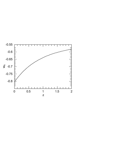
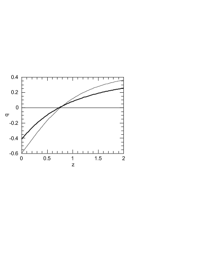
From the (22) we know directly that to explain the speeding up of the universe’s expansion as implied by lots of astrophysics observations, the effective state parameter for the vector field part’s contributions today must be smaller than $-\frac{2}{3}$ (instead of the $-\frac{1}{3}$ as given directly from the standard Friedmann equations for the $\Lambda$CDM model).

IV Current Observational Data

IV.1 Type Ia Supernovae

The observations of Type Ia supernovae (SNe Ia) provide an excellent tool for probing the expansion history of the universe. Because all type Ia supernovae explode at about the same mass, their absolute magnitudes are considered to be all the same ($M\thickapprox-19.3\pm 0.3$). This makes them very useful as standard candles. The observation of supernovae measure essentially the apparent magnitude $m$. The theoretical distance modulus is defined as

$$\mu_{th}=m_{th}-M=5\log_{10}D_{L}(z)+\mu_{0},$$ (23)

where $D_{L}(z)\equiv H_{0}d_{L}(z)$ is the dimensionless luminosity and $\mu_{0}=42.38-5\log_{10}h$. Here $h$ is the dimensionless Hubble parameter toady. $D_{L}(z)$ is given by

$$D_{L}(z)=\frac{1+z}{\sqrt{\Omega_{k}}}\sinh\left[H_{0}\sqrt{\Omega_{k}}\int^{z}_{0}\frac{dz^{\prime}}{H(z)}\right],$$ (24)

where $\Omega_{k}$ is the fractional curvature density today. In this paper we use the Union2 data set consisting of 557 supernovae. The corresponding $\chi^{2}_{SN}$ function to be minimized is

$$\chi^{2}_{SN}=\sum_{i=1}^{557}\left[\frac{\mu_{obs}(z_{i})-\mu_{th}(z_{i};{\bf\theta})}{\sigma_{i}}\right]^{2},$$ (25)

where ${\bf\theta}$ denotes the model parameters. The minimization with respect to $\mu_{0}$ can be made trivially by expanding $\chi^{2}_{SN}$ with respect to $\mu_{0}$ as Nesseris:2005ur

$$\chi^{2}_{SN}({\bf\theta})=A-2\mu_{0}B+\mu_{0}^{2}C,$$ (26)

where

$$A({\bf\theta}) = \sum_{i=1}^{557}\frac{[\mu_{obs}(z_{i})-\mu_{th}(z_{i};\mu_{0}=0,{\bf\theta})]^{2}}{\sigma_{i}^{2}}$$ (27)

$$B({\bf\theta}) = \sum_{i=1}^{557}\frac{\mu_{obs}(z_{i})-\mu_{th}(z_{i};\mu_{0}=0,{\bf\theta})}{\sigma_{i}^{2}}$$ (28)

$$C = \sum_{i=1}^{557}\frac{1}{\sigma_{i}^{2}}.$$ (29)

Equation (26) has a minimum for $\mu_{0}=B/C$ at

$$\tilde{\chi}^{2}_{SN}({\bf\theta})=A({\bf\theta})-\frac{B^{2}({\bf\theta})}{C}.$$ (30)

Thus instead of minimizing $\chi^{2}_{SN}$ we can minimize $\tilde{\chi}^{2}_{SN}$ which is independent of $\mu_{0}$.

IV.2 Cosmic Microwave Background and Baryonic Acoustic Oscillations

In addition to the type Ia supernovae data, we use the Cosmic Microwave Background (CMB) shift parameter and the Baryonic Acoustic Oscillations to compute the joint constraints. The shift parameter ${\cal R}$ is defined in Bond:1997wr as

$${\cal R}\equiv\sqrt{\Omega_{m}H^{2}_{0}}(1+z_{*})D_{A}(z_{*}),$$ (31)

where $z_{*}$ is the redshift of recombination and $D_{A}(z)$ is the proper angular diameter distance:

$$D_{A}(z)=\frac{1}{H_{0}(1+z)\sqrt{\Omega_{k}}}\sinh\left[H_{0}\sqrt{\Omega_{k}}\int^{z}_{0}\frac{dz^{\prime}}{H(z)}\right].$$ (32)

The seven-year WMAP results Komatsu:2010fb have updated the redshift of recombination $z_{*}=1091.3$ and the shift parameter ${\cal R}=1.725\pm 0.018$. The $\chi^{2}$ for CMB shift is

$$\chi^{2}_{CMB}({\bf\theta})=\frac{[{\cal R}({\bf\theta})-1.725]^{2}}{0.018^{2}}$$ (33)

Another constraint is from the Baryonic Acoustic Oscillations (BAOs) traced by the Sloan Digital Sky Survey (SDSS). In this paper we use only one node at $z=0.35$. The distance parameter ${\cal A}$ is defined asEisenstein:2005su

$${\cal A}\equiv D_{V}(0.35)\frac{\sqrt{\Omega_{m}H_{0}^{2}}}{0.35},$$ (34)

where $D_{V}$ is the effective distance

$$D_{V}(z)=\left[(1+z)^{2}D_{A}^{2}(z)\frac{z}{H(z)}\right]^{\frac{1}{3}}.$$ (35)

The value of ${\cal A}$ is given in Eisenstein:2005su : ${\cal A}=0.469\pm 0.017$. Thus the $\chi^{2}$ for BAO is

$$\chi^{2}_{BAO}({\bf\theta})=\frac{[{\cal A}({\bf\theta})-0.469]^{2}}{0.017^{2}}.$$ (36)

To compute the joint constraints, we add these $\chi^{2}$ functions together:

$$\chi^{2}=\tilde{\chi}_{SN}^{2}+\chi_{CMB}^{2}+\chi_{BAO}^{2}.$$ (37)

IV.3 Observational Hubble Parameter Data

There are two major methods of independent observational $H(z)$ measurement, which are called the “differential age method” and the “radial BAO size method”. The details can be found in Zhang:2010ic . In that paper, Tong-Jie Zhang and Cong Ma summarize the up-to-date observational Hubble parameter data (OHD). See below in Table 1. The data points at $z=0.24$ and $z=0.43$ are derived from the “radial BAO size method”, while the others are derived from the “differential age method” as named.

The $\chi^{2}$ for OHD is

$$\chi_{OHD}^{2}=\sum_{i=0}^{13}\frac{[H_{0}E(z_{i})-H_{obs}(z_{i})]^{2}}{\sigma_{i}^{2}},$$ (38)

where $E(z)\equiv H(z)/H_{0}$ is independent of $H_{0}$. Using the same trick mentioned before, the minimization with respect to $H_{0}$ can be made trivially by expanding $\chi^{2}_{OHD}$ with respect to $H_{0}$ as

$$\chi^{2}_{OHD}({\bf\theta})=H_{0}^{2}A-2H_{0}B+C,$$ (39)

where

$$A = \sum_{i=1}^{13}\frac{E^{2}(z_{i})}{\sigma_{i}^{2}}$$ (40)

$$B = \sum_{i=1}^{13}\frac{E(z_{i})H_{obs}(z_{i})}{\sigma_{i}^{2}}$$ (41)

$$C = \sum_{i=1}^{13}\frac{H_{obs}^{2}(z_{i})}{\sigma_{i}^{2}}.$$ (42)

Equation (39) has a minimum for $H_{0}=B/A$ at

$$\tilde{\chi}^{2}_{OHD}=-\frac{B^{2}}{A}+C.$$ (43)

Thus, instead of minimizing $\chi^{2}_{OHD}$ we can minimize $\tilde{\chi}^{2}_{OHD}$ which is independent of $H_{0}$. From Table 1, we can see the errors of OHD (data sets) listed are relatively larger. So we do analysis only with the OHD (data sets) separately with the hope that we can obtain more accuracy OHD in the near future.

Table 1: The set of available observational $H(z)$ data

$~{}~{}~{}~{}~{}~{}z~{}~{}~{}~{}~{}~{}$	$~{}~{}~{}~{}~{}~{}H(z)\pm 1\sigma~{}~{}~{}~{}~{}~{}$	References
	km s-1Mpc-1
0.09	$69\pm 12$	Jimenez:2003iv ; Stern:2009ep
0.17	$83\pm 8$	Stern:2009ep
0.24	$79.69\pm 2.65$	Gaztanaga:2008xz
0.27	$77\pm 14$	Stern:2009ep
0.4	$95\pm 17$	Stern:2009ep
0.43	$86.45\pm 3.68$	Gaztanaga:2008xz
0.48	$97\pm 62$	Stern:2009ep
0.88	$90\pm 40$	Stern:2009ep
0.9	$117\pm 23$	Stern:2009ep
1.3	$168\pm 17$	Stern:2009ep
1.43	$177\pm 18$	Stern:2009ep
1.53	$140\pm 14$	Stern:2009ep
1.75	$202\pm 40$	Stern:2009ep

V Results

For the $\Lambda$CDM model, the general expression for the expansion relation can be directly written out as

$$H(z)=H_{0}\sqrt{\Omega_{\Lambda}+\Omega_{k}(1+z)^{2}+\Omega_{m}(1+z)^{3}+\Omega_{R}(1+z)^{4}},$$ (44)

where $\Omega_{\Lambda}$, $\Omega_{k}$, $\Omega_{m}$, $\Omega_{R}$ are the fractional density of vacuum, curvature, matter and radiation today, respectively.

$$\Omega_{\Lambda}\equiv\frac{8\pi\Lambda}{3H_{0}^{2}},\quad\quad\Omega_{k}\equiv\frac{-k}{a_{0}^{2}H_{0}^{2}},\quad\quad\Omega_{m}\equiv\frac{8\pi\rho_{m}}{3H_{0}^{2}},\quad\quad\Omega_{R}\equiv\frac{8\pi\rho_{R}}{3H_{0}^{2}}\quad\quad.$$ (45)

In this paper, we fix $\Omega_{R}=\Omega_{\gamma}(1+0.2271N_{eff})$ and take the present photon density parameter $\Omega_{\gamma}=2.469\times 10^{-5}h^{-2}$ (for $T_{cmb}=2.725K$) and the effective number of neutrino species at its standard value 3.04 Komatsu:2010fb . We also use the prior $h=74.2\pm 3.6$ given in Riess:2009pu . So there are only two independent parameters $\Omega_{\Lambda}$ and $\Omega_{m}$. The parameter $\Omega_{k}$ can be expressed by the others:

$$\Omega_{k}=1-\Omega_{\Lambda}-\Omega_{m}-\Omega_{R}.$$ (46)

For the Einstein-aether theory with our choice of the free function ${\cal F}({\cal K})$, we can solve $H(z)$ from (20):

$$H(z)=H_{0}\left[\frac{\Omega_{A}}{2}+\sqrt{\frac{\Omega_{A}^{2}}{4}+\Omega_{k}(1+z)^{2}+\Omega_{m}(1+z)^{3}+\Omega_{R}(1+z)^{4}}\right],$$ (47)

where we define

$$\Omega_{A}\equiv\frac{M}{H_{0}}.$$ (48)

There are also only two parameters $\Omega_{A}$ and $\Omega_{m}$. Similarly, $\Omega_{k}$ can be expressed as (46), in which $\Omega_{\Lambda}$ needs to be replaced by $\Omega_{A}$.

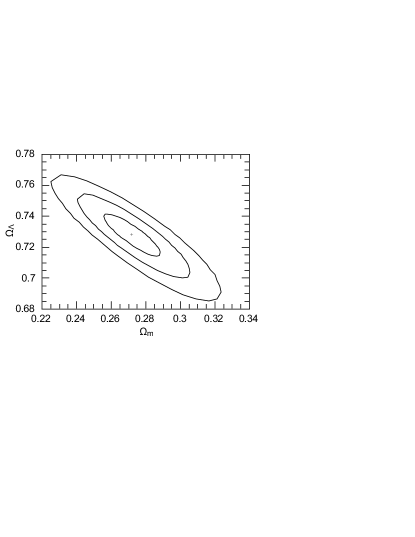
Firstly, we compute the combined constraints from SNe Ia, CMB shift and BAO data sets. The results are shown in Table 2 and Figure 1. The best-fit values for parameters of the $\Lambda$CDM model are consistent with the results given by WMAP 7 Jarosik:2010iu . It gives a nearly flat universe geometry with a tiny $\Omega_{k}=4\times 10^{-5}$. For the Einstein-aether theory case as we choose, the best-fit $\Omega_{m}$ is a little bit smaller than that in $\Lambda$CDM model, but it gives a larger $\Omega_{k}=0.04$. The $\Lambda$CDM model fits better to the data sets as its $\chi_{min}^{2}$ is $26.182$ smaller than that of Einstein-aether theory case as shown.

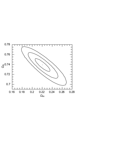
Then, we do similar analysis with the OHD (data sets). The results are shown in Table 2 and Figure 2 as well. This time, we can see that the Einstein-aether theory case fits a little better to the data sets, and the difference of the $\chi_{min}^{2}$ is very small now.

Noting the similarity of our modified Friedmann equation to that in DGP brane world model and data analysis being done to DGP model Li:2009jx ; Wan:2007pm , these result are rather natural, because best-fit $\Omega_{k}$ is very small.

Table 2: Best-fit parameters for $\Lambda$CDM model and Einstein-aether theory

	Model	Best-fit parameters	$\chi^{2}_{min}$
SN Ia-CMB shift-BAO	$\Lambda$CDM	$\Omega_{m}=0.272$	542.693
		$\Omega_{\Lambda}=0.728$
	Einstein-aether theory	$\Omega_{m}=0.220$	568.875
		$\Omega_{A}=0.739$
OHD	$\Lambda$CDM	$\Omega_{m}=0.322$	8.046
		$\Omega_{\Lambda}=0.807$
	Einstein-aether theory	$\Omega_{m}=0.301$	7.989
		$\Omega_{A}=1.040$

Figure 1: Joint constraints from SNe Ia, CMB shift and BAO. The $1\sigma$, $2\sigma$, $3\sigma$ confidence interval contours of $\Omega_{m}$ and $\Omega_{\Lambda}$ (or $\Omega_{A}$ for the Einstein-aether theory case) in $\Lambda$CDM model (left) and the Einstein-aether theory case(right).

Figure 2: Constraints from OHD. The $1\sigma$, $2\sigma$, $3\sigma$ confidence interval contours of $\Omega_{m}$ and $\Omega_{\Lambda}$ (or $\Omega_{A}$ for Einstein-aether theory case) in $\Lambda$CDM model (left) and Einstein-aether theory case (right).

Using the results of combined analysis we also plot the effective state parameter of the vector field part’s contribution $w_{A}(z)$ (Figure 3) and the corresponding deceleration parameter $q(z)$ (Figure 4), for demonstration.

Figure 3: The effective state parameter of the vector field part’s contribution.

Figure 4: The deceleration parameter. The thick solid line is the result of the Einstein-aether theory, while the thin dashed line represents $\Lambda$CDM model.

VI Conclusions and Discussions

In this paper we only consider in details a specific case of generalized Einstein-aether theories and compute the joint constraints from observations such as SNe Ia, CMB shift, BAO data sets, and OHD respectively. Even though we only investigate a specific case of generalized Einstein-aether model, we already see that it has shown lots of interesting features, by well fitting to the combined data sets of the SNe Ia, CMB shift and BAO, as well as OHD respectively, and comparing with the $\Lambda$CDM model.

The observational Hubble parameter data we have possessed now are relatively few and not so accurate. However, with the improving quality of observational $H(z)$ data and more data points being measured (more sample compiled hopefully), it will be certainly a directly useful tool to test dark energy models and modified theories of general relativity, as well as corresponding cosmology models.

For the case we analyze in this paper, the modified Friedmann equation is similar to that in DGP brane world model. It may be caused by the special ${\cal F}({\cal K})$ we choose. It looks first rather strange if there is any possible relation between these two theories, because the Einstein-aether theory is initially proposed for possible Lorentz violation and preferred frame effects, while the DGP brane world model considers a 3-brane embedded in a 5D bulk space-time. However, it is not completely impossible now.

Moreover, it is clearly shown in this special model that $M=\Omega_{A}H_{0}\thicksim H_{0}$, which is consistent with the requirements of MOND limit Zlosnik:2006zu ; Zlosnik:2007bu ; Zuntz:2010jp . However, further work needs to be elaborated on the stability analysis of this specific case we have considered.

For the last point of this present work we would like to make (but not the least importance), we should emphasize especially that theoretically we can not give for granted that the phenomenological MOND theory can reproduce all the systematics of Rotational Curves (RCs) observations, although the MOND model fits BETTER than the $\Lambda$CDM based mass models. It is still far away to reproduce the wide and far telling systematics of the spiral galaxies’ RCs (and of the mass distribution in the corresponding galaxies) sal , so there will be lots of detail work to be done with any modified gravity proposals at least on the galaxy scale.