ShareBoost: Efficient Multiclass Learning with Feature Sharing

Abstract

Multiclass prediction is the problem of classifying an object into a relevant target class. We consider the problem of learning a multiclass predictor that uses only few features, and in particular, the number of used features should increase sub-linearly with the number of possible classes. This implies that features should be shared by several classes. We describe and analyze the ShareBoost algorithm for learning a multiclass predictor that uses few shared features. We prove that ShareBoost efficiently finds a predictor that uses few shared features (if such a predictor exists) and that it has a small generalization error. We also describe how to use ShareBoost for learning a non-linear predictor that has a fast evaluation time. In a series of experiments with natural data sets we demonstrate the benefits of ShareBoost and evaluate its success relatively to other state-of-the-art approaches.

1 Introduction

Learning to classify an object into a relevant target class surfaces in many domains such as document categorization, object recognition in computer vision, and web advertisement. In multiclass learning problems we use training examples to learn a classifier which will later be used for accurately classifying new objects. Typically, the classifier first calculates several features from the input object and then classifies the object based on those features. In many cases, it is important that the runtime of the learned classifier will be small. In particular, this requires that the learned classifier will only rely on the value of few features.

We start with predictors that are based on linear combinations of features. Later, in Section 4, we show how our framework enables learning highly non-linear predictors by embedding non-linearity in the construction of the features. Requiring the classifier to depend on few features is therefore equivalent to sparseness of the linear weights of features. In recent years, the problem of learning sparse vectors for linear classification or regression has been given significant attention. While, in general, finding the most accurate sparse predictor is known to be NP hard [25, 10], two main approaches have been proposed for overcoming the hardness result. The first approach uses $\ell_{1}$ norm as a surrogate for sparsity (e.g. the Lasso algorithm [34] and the compressed sensing literature [6, 12]). The second approach relies on forward greedy selection of features (e.g. Boosting [16] in the machine learning literature and orthogonal matching pursuit in the signal processing community [36]).

A popular model for multiclass predictors maintains a weight vector for each one of the classes. In such case, even if the weight vector associated with each class is sparse, the overall number of used features might grow with the number of classes. Since the number of classes can be rather large, and our goal is to learn a model with an overall small number of features, we would like that the weight vectors will share the features with non-zero weights as much as possible. Organizing the weight vectors of all classes as rows of a single matrix, this is equivalent to requiring sparsity of the columns of the matrix.

In this paper we describe and analyze an efficient algorithm for learning a multiclass predictor whose corresponding matrix of weights has a small number of non-zero columns. We formally prove that if there exists an accurate matrix with a number of non-zero columns that grows sub-linearly with the number of classes, then our algorithm will also learn such a matrix. We apply our algorithm to natural multiclass learning problems and demonstrate its advantages over previously proposed state-of-the-art methods.

Our algorithm is a generalization of the forward greedy selection approach to sparsity in columns. An alternative approach, which has recently been studied in [28, 13], generalizes the $\ell_{1}$ norm based approach, and relies on mixed-norms. We discuss the advantages of the greedy approach over mixed-norms in Section 1.2.

1.1 Formal problem statement

Let $\mathcal{V}$ be the set of objects we would like to classify. For example, $\mathcal{V}$ can be the set of gray scale images of a certain size. For each object ${\mathbf{v}}\in\mathcal{V}$, we have a pool of predefined $d$ features, each of which is a real number in $[-1,1]$. That is, we can represent each ${\mathbf{v}}\in\mathcal{V}$ as a vector of features ${\mathbf{x}}\in[-1,1]^{d}$. We note that the mapping from ${\mathbf{v}}$ to ${\mathbf{x}}$ can be non-linear and that $d$ can be very large. For example, we can define ${\mathbf{x}}$ so that each element $x_{i}$ corresponds to some patch, $p\in\{\pm 1\}^{q\times q}$, and a threshold $\theta$, where $x_{i}$ equals $1$ if there is a patch of ${\mathbf{v}}$ whose inner product with $p$ is higher than $\theta$. We discuss some generic methods for constructing features in Section 4. From this point onward we assume that ${\mathbf{x}}$ is given.

The set of possible classes is denoted by $\mathcal{Y}=\{1,\ldots,k\}$. Our goal is to learn a multiclass predictor, which is a mapping from the features of an object into $\mathcal{Y}$. We focus on the set of predictors parametrized by matrices $W\in\mathbb{R}^{k,d}$ that takes the following form:

$$h_{W}({\mathbf{x}})=\operatorname*{argmax}_{y\in\mathcal{Y}}(W{\mathbf{x}})_{y}~{}.$$ (1)

That is, the matrix $W$ maps each $d$-dimensional feature vector into a $k$-dimensional score vector, and the actual prediction is the index of the maximal element of the score vector. If the maximizer is not unique, we break ties arbitrarily.

Recall that our goal is to find a matrix $W$ with few non-zero columns. We denote by $W_{\cdot,i}$ the $i$’th column of $W$ and use the notation

$$\|W\|_{\infty,0}=|\{i:\|W_{\cdot,i}\|_{\infty}>0\}|$$

to denote the number of columns of $W$ which are not identically the zero vector. More generally, given a matrix $W$ and a pair of norms $\|\cdot\|_{p},\|\cdot\|_{r}$ we denote $\|W\|_{p,r}=\left\|(\|W_{\cdot,1}\|_{p},\ldots,\|W_{\cdot,d}\|_{p})\right\|_{r}$, that is, we apply the $p$-norm on the columns of $W$ and the $r$-norm on the resulting $d$-dimensional vector.

The $0\!\!-\!\!1$ loss of a multiclass predictor $h_{W}$ on an example $({\mathbf{x}},y)$ is defined as $\boldsymbol{1}\!\left[h_{W}({\mathbf{x}})\neq y\right]$. That is, the $0\!\!-\!\!1$ loss equals $1$ if $h_{W}({\mathbf{x}})\neq y$ and $0$ otherwise. Since this loss function is not convex with respect to $W$, we use a surrogate convex loss function based on the following easy to verify inequalities:

$$\boldsymbol{1}[h_{W}({\mathbf{x}})\neq y] \leq\boldsymbol{1}\!\left[h_{W}({\mathbf{x}})\neq y\right]-(W{\mathbf{x}})_{y}+(W{\mathbf{x}})_{h_{W}({\mathbf{x}})}$$

$$\leq\max_{y^{\prime}\in\mathcal{Y}}\boldsymbol{1}\!\left[y^{\prime}\neq y\right]-(W{\mathbf{x}})_{y}+(W{\mathbf{x}})_{y^{\prime}}$$ (2)

$$\leq\ln\sum_{y^{\prime}\in\mathcal{Y}}e^{\boldsymbol{1}\!\left[y^{\prime}\neq y\right]-(W{\mathbf{x}})_{y}+(W{\mathbf{x}})_{y^{\prime}}}~{}.$$ (3)

We use the notation $\ell(W,({\mathbf{x}},y))$ to denote the right-hand side (eqn. (3)) of the above. The loss given in eqn. (2) is the multi-class hinge loss [8] used in Support-Vector-Machines, whereas $\ell(W,({\mathbf{x}},y))$ is the result of performing a “soft-max” operation: $\max_{x}f(x)\leq(1/p)\ln\sum_{x}e^{pf(x)}$, where equality holds for ${p\rightarrow\infty}$.

This logistic multiclass loss function $\ell(W,({\mathbf{x}},y))$ has several nice properties — see for example [40]. Besides being a convex upper-bound on the $0\!\!-\!\!1$ loss, it is smooth. The reason we need the loss function to be both convex and smooth is as follows. If a function is convex, then its first order approximation at any point gives us a lower bound on the function at any other point. When the function is also smooth, the first order approximation gives us both lower and upper bounds on the value of the function at any other point. ShareBoost uses the gradient of the loss function at the current solution (i.e. the first order approximation of the loss) to make a greedy choice of which column to update. To ensure that this greedy choice indeed yields a significant improvement we must know that the first order approximation is indeed close to the actual loss function, and for that we need both lower and upper bounds on the quality of the first order approximation.

Given a training set $S=({\mathbf{x}}_{1},y_{1}),\ldots,({\mathbf{x}}_{m},y_{m})$, the average training loss of a matrix $W$ is: $L(W)=\frac{1}{m}\sum_{({\mathbf{x}},y)\in S}\ell(W,({\mathbf{x}},y)).$ We aim at approximately solving the problem

$$\min_{W\in\mathbb{R}^{k,d}}L(W)~{}~{}~{}\textrm{s.t.}~{}~{}\|W\|_{\infty,0}\leq s~{}.$$ (4)

That is, find the matrix $W$ with minimal training loss among all matrices with column sparsity of at most $s$, where $s$ is a user-defined parameter. Since $\ell(W,({\mathbf{x}},y))$ is an upper bound on $\boldsymbol{1}\!\left[h_{W}({\mathbf{x}})\neq y\right]$, by minimizing $L(W)$ we also decrease the average $0\!\!-\!\!1$ error of $W$ over the training set. In Section 5 we show that for sparse models, a small training error is likely to yield a small error on unseen examples as well.

Regrettably, the constraint $\|W\|_{\infty,0}\leq s$ in eqn. (4) is non-convex, and solving the optimization problem in eqn. (4) is NP-hard [25, 10]. To overcome the hardness result, the ShareBoost algorithm will follow the forward greedy selection approach. The algorithm comes with formal generalization and sparsity guarantees (described in Section 5) that makes ShareBoost an attractive multiclass learning engine due to efficiency (both during training and at test time) and accuracy.

1.2 Related Work

The centrality of the multiclass learning problem has spurred the development of various approaches for tackling the task. Perhaps the most straightforward approach is a reduction from multiclass to binary, e.g. the one-vs-rest or all pairs constructions. The more direct approach we choose, in particular, the multiclass predictors of the form given in eqn. (1), has been extensively studied and showed a great success in practice — see for example [14, 38, 8].

An alternative construction, abbreviated as the single-vector model, shares a single weight vector, for all the classes, paired with class-specific feature mappings. This construction is common in generalized additive models [18], multiclass versions of boosting [17, 29], and has been popularized lately due to its role in prediction with structured output where the number of classes is exponentially large (see e.g. [32]). While this approach can yield predictors with a rather mild dependency of the required features on $k$ (see for example the analysis in [40, 32, 15]), it relies on a-priori assumptions on the structure of $\mathcal{X}$ and $\mathcal{Y}$. In contrast, in this paper we tackle general multiclass prediction problems, like object recognition or document classification, where it is not straightforward or even plausible how one would go about to construct a-priori good class specific feature mappings, and therefore the single-vector model is not adequate.

The class of predictors of the form given in eqn. (1) can be trained using Frobenius norm regularization (as done by multiclass SVM – see e.g. [8]) or using $\ell_{1}$ regularization over all the entries of $W$. However, as pointed out in [28], these regularizers might yield a matrix with many non-zeros columns, and hence, will lead to a predictor that uses many features.

The alternative approach, and the most relevant to our work, is the use of mix-norm regularizations like $\|W\|_{\infty,1}$ or $\|W\|_{2,1}$ [22, 37, 2, 3, 28, 13, 20]. For example, [13] solves the following problem:

$$\min_{W\in\mathbb{R}^{k,d}}L(W)+\lambda\|W\|_{\infty,1}~{}.$$ (5)

which can be viewed as a convex approximation of our objective (eqn. (4)). This is advantageous from an optimization point of view, as one can find the global optimum of a convex problem, but it remains unclear how well the convex program approximates the original goal. For example, in Section 6 we show cases where mix-norm regularization does not yield sparse solutions while ShareBoost does yield a sparse solution. Despite the fact that ShareBoost tackles a non-convex program, and thus limited to local optimum solutions, we prove in Theorem 2 that under mild conditions ShareBoost is guaranteed to find an accurate sparse solution whenever such a solution exists and that the generalization error is bounded as shown in Theorem 1.

We note that several recent papers (e.g. [20]) established exact recovery guarantees for mixed norms, which may seem to be stronger than our guarantee given in Theorem 2. However, the assumptions in [20] are much stronger than the assumptions of Theorem 2. In particular, they have strong noise assumptions and a group RIP like assumption (Assumption 4.1-4.3 in their paper). In contrast, we impose no such restrictions. We would like to stress that in many generic practical cases, the assumptions of [20] will not hold. For example, when using decision stumps, features will be highly correlated which will violate Assumption 4.3 of [20].

Another advantage of ShareBoost is that its only parameter is the desired number of non-zero columns of $W$. Furthermore, obtaining the whole-regularization-path of ShareBoost, that is, the curve of accuracy as a function of sparsity, can be performed by a single run of ShareBoost, which is much easier than obtaining the whole regularization path of the convex relaxation in eqn. (5). Last but not least, ShareBoost can work even when the initial number of features, $d$, is very large, as long as there is an efficient way to choose the next feature. For example, when the features are constructed using decision stumps, $d$ will be extremely large, but ShareBoost can still be implemented efficiently. In contrast, when $d$ is extremely large mix-norm regularization techniques yield challenging optimization problems.

As mentioned before, ShareBoost follows the forward greedy selection approach for tackling the hardness of solving eqn. (4). The greedy approach has been widely studied in the context of learning sparse predictors for linear regression. However, in multiclass problems, one needs sparsity of groups of variables (columns of $W$). ShareBoost generalizes the fully corrective greedy selection procedure given in [30] to the case of selection of groups of variables, and our analysis follows similar techniques.

Obtaining group sparsity by greedy methods has been also recently studied in [21, 24], and indeed, ShareBoost shares similarities with these works. We differ from [21] in that our analysis does not impose strong assumptions (e.g. group-RIP) and so ShareBoost applies to a much wider array of applications. In addition, the specific criterion for choosing the next feature is different. In [21], a ratio between difference in objective and different in costs is used. In ShareBoost, the L1 norm of the gradient matrix is used. For the multiclass problem with log loss, the criterion of ShareBoost is much easier to compute, especially in large scale problems. [24] suggested many other selection rules that are geared toward the squared loss, which is far from being an optimal loss function for multiclass problems.

Another related method is the JointBoost algorithm [35]. While the original presentation in [35] seems rather different than the type of predictors we describe in eqn. (1), it is possible to show that JointBoost in fact learns a matrix $W$ with additional constraints. In particular, the features ${\mathbf{x}}$ are assumed to be decision stumps and each column $W_{\cdot,i}$ is constrained to be $\alpha_{i}(\boldsymbol{1}\!\left[1\in C_{i}\right],\ldots,\boldsymbol{1}\!\left[k\in C_{i}\right])$, where $\alpha_{i}\in\mathbb{R}$ and $C_{i}\subset\mathcal{Y}$. That is, the stump is shared by all classes in the subset $C_{i}$. JointBoost chooses such shared decision stumps in a greedy manner by applying the GentleBoost algorithm on top of this presentation. A major disadvantage of JointBoost is that in its pure form, it should exhaustively search $C$ among all $2^{k}$ possible subsets of $\mathcal{Y}$. In practice, [35] relies on heuristics for finding $C$ on each boosting step. In contrast, ShareBoost allows the columns of $W$ to be any real numbers, thus allowing ”soft” sharing between classes. Therefore, ShareBoost has the same (or even richer) expressive power comparing to JointBoost. Moreover, ShareBoost automatically identifies the relatedness between classes (corresponding to choosing the set $C$) without having to rely on exhaustive search. ShareBoost is also fully corrective, in the sense that it extracts all the information from the selected features before adding new ones. This leads to higher accuracy while using less features as was shown in our experiments on image classification. Lastly, ShareBoost comes with theoretical guarantees.

Finally, we mention that feature sharing is merely one way for transferring information across classes [33] and several alternative ways have been proposed in the literature such as target embedding [19, 5], shared hidden structure [23, 1], shared prototypes [27], or sharing underlying metric [39].

2 The ShareBoost Algorithm

ShareBoost is a forward greedy selection approach for solving eqn. (4). Usually, in a greedy approach, we update the weight of one feature at a time. Now, we will update one column of $W$ at a time (since the desired sparsity is over columns). We will choose the column that maximizes the $\ell_{1}$ norm of the corresponding column of the gradient of the loss at $W$. Since $W$ is a matrix we have that $\nabla L(W)$ is a matrix of the partial derivatives of $L$. Denote by $\nabla_{r}L(W)$ the $r$’th column of $\nabla L(W)$, that is, the vector $\left(\frac{\partial L(W)}{\partial W_{1,r}},\ldots,\frac{\partial L(W)}{\partial W_{k,r}}\right)$. A standard calculation shows that

$$\frac{\partial L(W)}{\partial W_{q,r}} =\frac{1}{m}\sum_{({\mathbf{x}},y)\in S}\sum_{c\in\mathcal{Y}}\rho_{c}({\mathbf{x}},y)\,x_{r}(\boldsymbol{1}\!\left[q=c\right]-\boldsymbol{1}\!\left[q=y\right])$$

where

$$\rho_{c}({\mathbf{x}},y)=\frac{e^{\boldsymbol{1}\!\left[c\neq y\right]-(W{\mathbf{x}})_{y}+(W{\mathbf{x}})_{c}}}{\sum_{y^{\prime}\in\mathcal{Y}}e^{\boldsymbol{1}\!\left[y^{\prime}\neq y\right]-(W{\mathbf{x}})_{y}+(W{\mathbf{x}})_{y^{\prime}}}}.$$ (6)

Note that $\sum_{c}\rho_{c}({\mathbf{x}},y)=1$ for all $({\mathbf{x}},y)$. Therefore, we can rewrite,

$$\frac{\partial L(W)}{\partial W_{q,r}} =\frac{1}{m}\sum_{({\mathbf{x}},y)}x_{r}(\rho_{q}({\mathbf{x}},y)-\boldsymbol{1}\!\left[q=y\right])~{}.$$

Based on the above we have

$$\|\nabla_{r}L(W)\|_{1}~{}=~{}\frac{1}{m}\sum_{q\in\mathcal{Y}}\left|\sum_{({\mathbf{x}},y)}x_{r}(\rho_{q}({\mathbf{x}},y)-\boldsymbol{1}\!\left[q=y\right])\right|~{}.$$ (7)

Finally, after choosing the column for which $\|\nabla_{r}L(W)\|_{1}$ is maximized, we re-optimize all the columns of $W$ which were selected so far. The resulting algorithm is given in Algorithm 1.

Algorithm 1 ShareBoost

1:  Initialize: $W=0$  ;  $I=\emptyset$

2:  for t=1,2,…,T do

3:     For each class $c$ and example $({\mathbf{x}},y)$ define $\rho_{c}({\mathbf{x}},y)$ as in eqn. (6)

4:     Choose feature $r$ that maximizes the right-hand side of eqn. (7)

5:     $I\leftarrow I\cup\{r\}$

6:     Set $W\leftarrow\operatorname*{argmin}_{W}L(W)$ s.t. $W_{\cdot,i}=\boldsymbol{0}$ for all $i\notin I$

7:  end for

The runtime of ShareBoost is as follows. Steps 3-5 requires $O(mdk)$. Step 6 is a convex optimization problem in $tk$ variables and can be performed using various methods. In our experiments, we used Nesterov’s accelerated gradient method [26] whose runtime is $O(mtk/\sqrt{\epsilon})$ for a smooth objective, where $\epsilon$ is the desired accuracy. Therefore, the overall runtime is $O(Tmdk+T^{2}mk/\sqrt{\epsilon})$. It is interesting to compare this runtime to the complexity of minimizing the mixed-norm regularization objective given in eqn. (5). Since the objective is no longer smooth, the runtime of using Nesterov’s accelerated method would be $O(mdk/\epsilon)$ which can be much larger than the runtime of ShareBoost when $d\gg T$.

3 Variants of ShareBoost

We now describe several variants of ShareBoost. The analysis we present in Section 5 can be easily adapted for these variants as well.

3.1 Modifying the Greedy Choice Rule

ShareBoost chooses the feature $r$ which maximizes the $\ell_{1}$ norm of the $r$-th column of the gradient matrix. Our analysis shows that this choice leads to a sufficient decrease of the objective function. However, one can easily develop other ways for choosing a feature which may potentially lead to an even larger decrease of the objective. For example, we can choose a feature $r$ that minimizes $L(W)$ over matrices $W$ with support of $I\cup\{r\}$. This will lead to the maximal possible decrease of the objective function at the current iteration. Of course, the runtime of choosing $r$ will now be much larger. Some intermediate options are to choose $r$ that minimizes

$$\min_{\alpha\in\mathbb{R}}W+\alpha\nabla_{r}R(W)$$

or to choose $r$ that minimizes

$$\min_{{\mathbf{w}}\in\mathbb{R}^{k}}W+{\mathbf{w}}{\mathbf{e}}_{r}^{\dagger},$$

where ${\mathbf{e}}_{r}^{\dagger}$ is the all-zero row vector except $1$ in the $r$’th position.

3.2 Selecting a Group of Features at a Time

In some situations, features can be divided into groups where the runtime of calculating a single feature in each group is almost the same as the runtime of calculating all features in the group. In such cases, it makes sense to choose groups of features at each iteration of ShareBoost. This can be easily done by simply choosing the group of features $J$ that maximizes $\sum_{j\in J}\|\nabla_{j}L(W)\|_{1}$.

3.3 Adding Regularization

Our analysis implies that when $|S|$ is significantly larger than $\tilde{O}(Tk)$ then ShareBoost will not overfit. When this is not the case, we can incorporate regularization in the objective of ShareBoost in order to prevent overfitting. One simple way is to add to the objective function $L(W)$ a Frobenius norm regularization term of the form $\lambda\sum_{i,j}W_{i,j}^{2}$, where $\lambda$ is a regularization parameter. It is easy to verify that this is a smooth and convex function and therefore we can easily adapt ShareBoost to deal with this regularized objective. It is also possible to rely on other norms such as the $\ell_{1}$ norm or the $\ell_{\infty}/\ell_{1}$ mixed-norm. However, there is one technicality due to the fact that these norms are not smooth. We can overcome this problem by defining smooth approximations to these norms. The main idea is to first note that for a scalar $a$ we have $|a|=\max\{a,-a\}$ and therefore we can rewrite the aforementioned norms using max and sum operations. Then, we can replace each max expression with its soft-max counterpart and obtain a smooth version of the overall norm function. For example, a smooth version of the $\ell_{\infty}/\ell_{1}$ norm will be $\|W\|_{\infty,1}\approx\frac{1}{\beta}\sum_{j=1}^{d}\log\left(\sum_{i=1}^{k}(e^{\beta W_{i,j}}+e^{-\beta W_{i,j}})\right)~{},$ where $\beta\geq 1$ controls the tradeoff between quality of approximation and smoothness.

4 Non-Linear Prediction Rules

We now demonstrate how ShareBoost can be used for learning non-linear predictors. The main idea is similar to the approach taken by Boosting and SVM. That is, we construct a non-linear predictor by first mapping the original features into a higher dimensional space and then learning a linear predictor in that space, which corresponds to a non-linear predictor over the original feature space. To illustrate this idea we present two concrete mappings. The first is the decision stumps method which is widely used by Boosting algorithms. The second approach shows how to use ShareBoost for learning piece-wise linear predictors and is inspired by the super-vectors construction recently described in [41].

4.1 ShareBoost with Decision Stumps

Let ${\mathbf{v}}\in\mathbb{R}^{p}$ be the original feature vector representing an object. A decision stump is a binary feature of the form $\boldsymbol{1}\!\left[v_{i}\leq\theta\right]$, for some feature $i\in\{1,\ldots,p\}$ and threshold $\theta\in\mathbb{R}$. To construct a non-linear predictor we can map each object ${\mathbf{v}}$ into a feature-vector ${\mathbf{x}}$ that contains all possible decision stumps. Naturally, the dimensionality of ${\mathbf{x}}$ is very large (in fact, can even be infinite), and calculating Step 4 of ShareBoost may take forever. Luckily, a simple trick yields an efficient solution. First note that for each $i$, all stump features corresponding to $i$ can get at most $m+1$ values on a training set of size $m$. Therefore, if we sort the values of $v_{i}$ over the $m$ examples in the training set, we can calculate the value of the right-hand side of eqn. (7) for all possible values of $\theta$ in total time of $O(m)$. Thus, ShareBoost can be implemented efficiently with decision stumps.

Figure 1: Motivating super vectors.

4.2 Learning Piece-wise Linear Predictors with ShareBoost

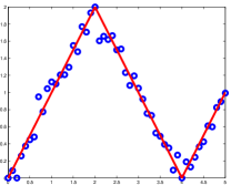
To motivate our next construction let us consider first a simple one dimensional function estimation problem. Given sample $(x_{1},y_{i}),\ldots,(x_{m},y_{m})$ we would like to find a function $f:\mathbb{R}\to\mathbb{R}$ such that $f(x_{i})\approx y_{i}$ for all $i$. The class of piece-wise linear functions can be a good candidate for the approximation function $f$. See for example an illustration in Fig. 1. In fact, it is easy to verify that all smooth functions can be approximated by piece-wise linear functions (see for example the discussion in [41]). In general, we can express piece-wise linear vector-valued functions as

$$f({\mathbf{v}})=\sum_{j=1}^{q}\boldsymbol{1}\!\left[\|{\mathbf{v}}-{\mathbf{v}}_{j}\|<r_{j}\right](\langle{\mathbf{u}}_{j},{\mathbf{v}}\rangle+b_{j})~{},$$

where $q$ is the number of pieces, $({\mathbf{u}}_{j},b_{j})$ represents the linear function corresponding to piece $j$, and $({\mathbf{v}}_{j},r_{j})$ represents the center and radius of piece $j$. This expression can be also written as a linear function over a different domain, $f({\mathbf{v}})=\langle{\mathbf{w}},\psi({\mathbf{v}})\rangle$ where

$$\psi({\mathbf{v}})=\left[\,\boldsymbol{1}\!\left[\|{\mathbf{v}}-{\mathbf{v}}_{1}\|<r_{1}\right][{\mathbf{v}}\,,\,1]\,,\,\ldots\,,\,\boldsymbol{1}\!\left[\|{\mathbf{v}}-{\mathbf{v}}_{q}\|<r_{q}\right][{\mathbf{v}}\,,\,1]\,\right]~{}.$$

In the case of learning a multiclass predictor, we shall learn a predictor ${\mathbf{v}}\mapsto W\psi({\mathbf{v}})$, where $W$ will be a $k$ by $\textrm{dim}(\psi({\mathbf{v}}))$ matrix. ShareBoost can be used for learning $W$. Furthermore, we can apply the variant of ShareBoost described in Section 3.2 to learn a piece-wise linear model which few pieces (that is, each group of features will correspond to one piece of the model). In practice, we first define a large set of candidate centers by applying some clustering method to the training examples, and second we define a set of possible radiuses by taking values of quantiles from the training examples. Then, we train ShareBoost so as to choose a multiclass predictor that only use few pairs $({\mathbf{v}}_{j},r_{j})$.

The advantage of using ShareBoost here is that while it learns a non-linear model it will try to find a model with few linear “pieces”, which is advantageous both in terms of test runtime as well as in terms of generalization performance.

5 Analysis

In this section we provide formal guarantees for the ShareBoost algorithm. The proofs are deferred to the appendix. We first show that if the algorithm has managed to find a matrix $W$ with a small number of non-zero columns and a small training error, then the generalization error of $W$ is also small. The bound below is in terms of the $0\!\!-\!\!1$ loss. A related bound, which is given in terms of the convex loss function, is described in [40].

Theorem 1

Suppose that the ShareBoost algorithm runs for $T$ iterations and let $W$ be its output matrix. Then, with probability of at least $1-\delta$ over the choice of the training set $S$ we have that

$$\operatorname*{\mathbb{P}}_{({\mathbf{x}},y)\sim\mathcal{D}}\left[h_{W}({\mathbf{x}})\neq y\right]\leq\operatorname*{\mathbb{P}}_{({\mathbf{x}},y)\sim S}\left[h_{W}({\mathbf{x}})\neq y\right]$$

$$+O\left(\sqrt{\frac{Tk\log(Tk)\log(k)+T\log(d)+\log(1/\delta)}{|S|}}\right)$$

Next, we analyze the sparsity guarantees of ShareBoost. As mentioned previously, exactly solving eqn. (4) is known to be NP hard. The following main theorem gives an interesting approximation guarantee. It tells us that if there exists an accurate solution with small $\ell_{\infty,1}$ norm, then the ShareBoost algorithm will find a good sparse solution.

Theorem 2

Let $\epsilon>0$ and let $W^{\star}$ be an arbitrary matrix. Assume that we run the ShareBoost algorithm for $T=\left\lceil 4\,\tfrac{1}{\epsilon}\,\|W^{\star}\|_{\infty,1}^{2}\right\rceil$ iterations and let $W$ be the output matrix. Then, $\|W\|_{\infty,0}\leq T$ and $L(W)\leq L(W^{\star})+\epsilon$.

6 Feature Sharing — Illustrative Examples

In this section we present illustrative examples, showing that whenever strong feature sharing is possible then ShareBoost will find it, while competitive methods might fail to produce solutions with a small number of features.

In the analysis of the examples below we use the following simple corollary of Theorem 2.

Corollary 1

Assume that there exists a matrix $W^{\star}$ such that $L(W^{\star})\leq\epsilon$, all entries of $W^{\star}$ are in $[-c,c]$, and $\|W^{\star}\|_{\infty,0}=r$. Then, ShareBoost will find a matrix $W$ with $L(W)\leq 2\epsilon$ and $\|W\|_{\infty,0}\leq 4r^{2}c^{2}/\epsilon$.

The first example we present shows an exponential gap between the number of features required by ShareBoost (as well as mixed norms) and the number of features required by $\ell_{2}$ or $\ell_{1}$ regularization methods. Consider a set of examples such that each example, $({\mathbf{x}},y)$, is of the form ${\mathbf{x}}=[\textrm{bin}(y),2\log(k)\,{\mathbf{e}}^{y}]\in\mathbb{R}^{\log(k)+k}$, where $\textrm{bin}(y)\in\{\pm 1\}^{\log(k)}$ is the binary representation of the number $y$ in the alphabet $\{\pm 1\}$ and ${\mathbf{e}}^{y}$ is the vector which is zero everywhere except $1$ in the $y$’th coordinate. For example, if $k=4$ then $\textrm{bin}(1)=[-1,1]$, $\textrm{bin}(2)=[1,-1]$, $\textrm{bin}(3)=[1,1]$, and $\textrm{bin}(4)=[-1,-1]$.

Consider two matrices. The first matrix, denoted $W^{(s)}$, is the matrix whose row $y$ equals to $[\textrm{bin}(y),(0,\ldots,0)]$. The second matrix, denoted $W^{(f)}$, is the matrix whose row $y$ equals to $[(0,\ldots,0),{\mathbf{e}}^{y}]$. Clearly, the number of features used by $h_{W^{(s)}}$ is $\log(k)$ while the number of features used by $h_{W^{(f)}}$ is $k$.

Observe that both $h_{W^{(f)}}({\mathbf{x}})$ and $h_{W^{(s)}}({\mathbf{x}})$ (see definition in eqn. (1)), will make perfect predictions on the training set. Furthermore, since for each example $({\mathbf{x}},y)$, for each $r\neq y$ we have that $(W^{(s)}{\mathbf{x}})_{r}\in[-\log(k),\log(k)-2]$, for the logistic multiclass loss, for any $c>0$ we have that

$$L(cW^{(f)}) =\log(1+(k-1)e^{1-2c\log(k)})$$

$$<L(cW^{(s)})$$

$$<\log(1+(k-1)e^{1-c(\log(k)-2)})~{}.$$

It follows that for

$$c\geq\frac{1+\log(k-1)-\log(e^{\epsilon}-1)}{\log(k)-2}$$

we have that $L(cW^{(s)})\leq\epsilon$.

Consider an algorithm that solves the regularized problem

$$\min_{W}L(W)+\lambda\,\|W\|_{p,p}~{},$$

where $p$ is either $1$ or $2$. In both cases, we have that $\|W^{(f)}\|_{p,p}<\|W^{(s)}\|_{p,p}$. It follows that for any value of $\lambda$, and for any $c>0$, the value of the objective at $cW^{(f)}$ is smaller than the value at $cW^{(s)}$. In fact, it is not hard to show that the optimal solution takes the form $cW^{(f)}$ for some $c>0$. Therefore, no matter what the regularization parameter $\lambda$ is, the solution of the above regularized problem will use $k$ features, even though there exists a rather good solution that relies on $\log(k)$ shared features.

In contrast, using Corollary 1 we know that if we stop ShareBoost after $\mathrm{poly}(\log(k))$ iterations it will produce a matrix that uses only $\mathrm{poly}(\log(k))$ features and has a small loss. Similarly, it is possible to show that for an appropriate regularization parameter, the mix-norm regularization $\|W\|_{\infty,1}$ will also yield the matrix $W^{(s)}$ rather than the matrix $W^{(f)}$.

In our second example we show that in some situations using the mix-norm regularization,

$$\min_{W}L(W)+\lambda\|W\|_{\infty,1}~{},$$

will also fail to produce a sparse solution, while ShareBoost is still guaranteed to learn a sparse solution. Let $s$ be an integer and consider examples $({\mathbf{x}},y)$ where each ${\mathbf{x}}$ is composed of $s$ blocks, each of which is in $\{\pm 1\}^{\log(k)}$. We consider two types of examples. In the first type, each block of ${\mathbf{x}}$ equals to $\textrm{bin}(y)$. In the second type, we generate example as in the first type, but then we zero one of the blocks (where we choose uniformly at random which block to zero). As before, $(1-\epsilon)m$ examples are of the first type while $\epsilon m$ examples are of the second type.

Consider again two matrices. The first matrix, denoted $W^{(s)}$, is the matrix whose row $y$ equals to $[\textrm{bin}(y),(0,\ldots,0)]$. The second matrix, denoted $W^{(f)}$, is the matrix whose row $y$ equals to $[\textrm{bin}(y),\ldots,\textrm{bin}(y)]/s$. Note that $\|W^{(f)}\|_{\infty,1}=\|W^{(s)}\|_{\infty,1}$. In addition, for any $({\mathbf{x}},y)$ of the second type we have that $\mathbb{E}[W^{(s)}{\mathbf{x}}]=W^{(f)}{\mathbf{x}}$, where expectation is with respect to the choice of which block to zero. Since the loss function is strictly convex, it follows from Jensen’s inequality that $L(W^{(f)})<L(W^{(s)})$. We have thus shown that using the $(\infty,1)$ mix-norm as a regularization will prefer the matrix $W^{(f)}$ over $W^{(s)}$. In fact, it is possible to show that the minimizer of $L(W)+\lambda\|W\|_{\infty,1}$ will be of the form $cW^{(f)}$ for some $c$. Since the number of blocks, $s$, was arbitrarily large, and since ShareBoost is guaranteed to learn a matrix with at most $\mathrm{poly}(\log(k))$ non-zero columns, we conclude that there can be a substantial gap between mix-norm regularization and ShareBoost. The advantage of ShareBoost in this example follows from its ability to break ties (even in an arbitrary way).

Naturally, the aforementioned examples are synthetic and capture extreme situations. However, in our experiments below we show that ShareBoost performs better than mixed-norm regularization on natural data sets as well.

7 Experiments

In this section we demonstrate the merits (and pitfalls) of ShareBoost by comparing it to alternative algorithms in different scenarios. The first experiment exemplifies the feature sharing property of ShareBoost. We perform experiments with an OCR data set and demonstrate a mild growth of the number of features as the number of classes grows from 2 to 36. The second experiment compares ShareBoost to mixed-norm regularization and to the JointBoost algorithm of [35]. We follow the same experimental setup as in [13]. The main finding is that ShareBoost outperforms the mixed-norm regularization method when the output predictor needs to be very sparse, while mixed-norm regularization can be better in the regime of rather dense predictors. We also show that ShareBoost is both faster and more accurate than JointBoost. The third and final set of experiments is on the MNIST handwritten digit dataset where we demonstrate state-of-the-art accuracy at extremely efficient runtime performance.

7.1 Feature Sharing

The main motivation for deriving the ShareBoost algorithm is the need for a multiclass predictor that uses only few features, and in particular, the number of features should increase slowly with the number of classes. To demonstrate this property of ShareBoost we experimented with the Char74k data set which consists of images of digits and letters. We trained ShareBoost with the number of classes varying from 2 classes to the 36 classes corresponding to the 10 digits and 26 capital letters. We calculated how many features were required to achieve a certain fixed accuracy as a function of the number of classes. The description of the feature space is described in Section 7.4.

Figure 2: The number of features required to achieve a fixed accuracy as a function of the number of classes for ShareBoost (dashed) and the 1-vs-rest (solid-circles). The blue lines are for a target error of 20% and the green lines are for 8%.

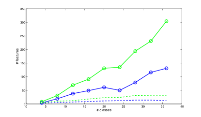
We compared ShareBoost to the 1-vs-rest approach, where in the latter, we trained each binary classifier using the same mechanism as used by ShareBoost. Namely, we minimize the binary logistic loss using a greedy algorithm. Both methods aim at constructing sparse predictors using the same greedy approach. The difference between the methods is that ShareBoost selects features in a shared manner while the 1-vs-rest approach selects features for each binary problem separately. In Fig. 2 we plot the overall number of features required by both methods to achieve a fixed accuracy on the test set as a function of the number of classes. As can be easily seen, the increase in the number of required features is mild for ShareBoost but significant for the 1-vs-rest approach.

7.2 Comparing ShareBoost to Mixed-Norms Regularization

Our next experiment compares ShareBoost to the use of mixed-norm regularization (see eqn. (5)) as a surrogate for the non-convex sparsity constraint. See Section 1.2 for description of the approach. To make the comparison fair, we followed the same experimental setup as in [13] (using code provided by ).

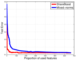
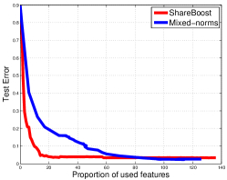
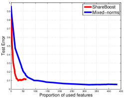
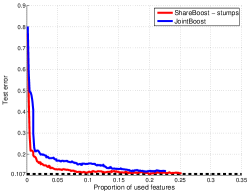
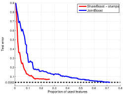
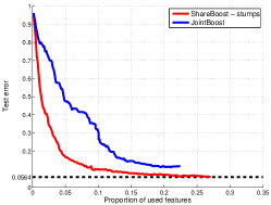
We calculated the whole regularization path for the mixed-norm regularization by running the algorithm of [13] with many values of the regularization parameter $\lambda$. In Fig. 3 we plot the results on three UCI datasets: StatLog, Pendigits and Isolet. The number of classes for the datasets are 7,10,26, respectively. The original dimensionality of these datasets is not very high and therefore, following [13], we expanded the features by taking all products over ordered pairs of features. After this transformation, the number of features were 630, 120, 190036, respectively.

Fig. 3 displays the results. As can be seen, ShareBoost decreases the error much faster than the mixed-norm regularization, and therefore is preferable when the goal is to have a rather sparse solution. When more features are allowed, ShareBoost starts to overfit. This is not surprising since here sparsity is our only mean for controlling the complexity of the learned classifier. To prevent this overfitting effect, one can use the variant of ShareBoost that incorporates regularization—see Section 3.

(a) StatLog	(b) Pendigits	(c) Isolet

Figure 3: ShareBoost compared with mixed-norm regularization (top) and JointBoost (bottom) on several UCI datasets. The horizontal axis is the feature sparsity (fraction of features used) and the vertical axis is the test error rate.

7.3 Comparing ShareBoost to JointBoost

Here we compare ShareBoost to the JointBoost algorithm of [35]. See Section 1.2 for description of JointBoost. As in the previous experiment, we followed the experimental setup as in [13] and ran JointBoost of [35] using their published code with additional implementation of the BFS heuristic for pruning the $2^{k}$ space of all class-subsets as described in their paper.

Fig. 3 (bottom) displays the results. Here we used stump features for both algorithms since these are needed for JointBoost. As can be seen, ShareBoost decreases the error much faster and therefore is preferable when the goal is to have a rather sparse solution. As in the previous experiment we observe that when more features are allowed, ShareBoost starts to overfit. Again, this is not surprising and can be prevented by adding additional regularization. The training runtime of ShareBoost is also much shorter than that of JointBoost (see discussion in Section 1.2).

Reference	3NN	Shape Context	SVM 9-poly	Neural Net	ShareBoost
		Belongie-et-al	DeCosta-et-al	Ciresan-et-al
Error rate	2.7%	0.63%	0.56%	0.35%	0.47%
Errors	270	63	56	35	47
Year	–	2002	2002	2010	2011
Run time	$\times$ 14	$\times$ 1000’s	$\times$ 38	$\times$ 2.5	1

Table 1: Comparison of ShareBoost and relevant methods on error rate and computational complexity over the MNIST dataset. More details in the text.

7.4 MNIST Handwritten Digits Dataset

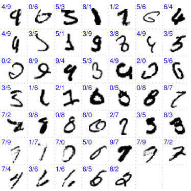
The goal of this experiment is to show that ShareBoost achieves state-of-the-art performance while constructing very fast predictors. We experimented with the MNIST digit dataset, which consists of a training set of $60,000$ digits represented by centered size-normalized $28\times 28$ images, and a test set of $10,000$ digits (see Fig. 6 for some examples). The MNIST dataset has been extensively studied and is considered the standard test for multiclass classification of handwritten digits. The error rate achieved by the most advanced algorithms are below $1\%$ of the test set (i.e., below $100$ classification mistakes on the test set). To get a sense of the challenge involved with the MNIST dataset, consider a straightforward 3-Nearest-Neighbor (3NN) approach where each test example ${\mathbf{x}}$, represented as a vector with $28^{2}$ entries, is matched against the entire training set ${\mathbf{x}}_{j}$ using the distance $d({\mathbf{x}},{\mathbf{x}}_{j})=\|{\mathbf{x}}-{\mathbf{x}}_{j}\|^{2}$. The classification decision is then the majority class label of the three most nearest training examples. This naive 3NN approach achieves an error rate of $2.67\%$ (i.e., $267$ mis-classification errors) with a run-time of unwieldy proportions. Going from 3NN to qNN with $q=4,...,12$ does not produce a better error rate.

More advanced shape-similarity measures could improve the performance of the naive $qNN$ approach but at a heavier run-time cost. For example, the Shape Context similarity measure introduced by [4] uses a Bipartite matching algorithm between descriptors computed along $100$ points in each image. A 3NN using Shape-Context similarity achieves an error rate of $0.63\%$ but at a very high (practically unwieldy) run-time cost. The challenge with the MNIST dataset is, therefore, to design a multiclass algorithm with a small error rate (say below $1\%$) and have an efficient run-time performance.

The top MNIST performer [7] uses a feed-forward Neural-Net with $7.6$ million connections which roughly translates to $7.6$ million multiply-accumulate (MAC) operations at run-time as well. During training, geometrically distorted versions of the original examples were generated in order to expand the training set following [31] who introduced a warping scheme for that purpose. The top performance error rate stands at $0.35\%$ at a run-time cost of $7.6$ million MAC per test example.

Table  1 summarizes the discussion so far including the performance of ShareBoost. The error-rate of ShareBoost with $266$ rounds stands on $0.71\%$ using the original training set and $0.47\%$ with the expanded training set of $360,000$ examples generated by adding five deformed instances per original example and with $T=305$ rounds. The run-time on test examples is around $40\%$ of the leading MNIST performer. The error rate of $0.47\%$ is better than that reported by [11] who used a 1-vs-all SVM with a 9-degree polynomial kernel and with an expanded training set of $780,000$ examples. The number of support vectors (accumulated over the ten separate binary classifiers) was $163,410$ giving rise to a run-time of $21$-fold compared to ShareBoost. We describe below the details of the ShareBoost implementation on the MNIST dataset.

The feature space we designed consists of 7$\times$7 image patches with corresponding spatial masks, constructed as follows. All 7$\times$7 patches were collected from all images and clustered using K-means to produce $1000$ centers $w_{f}$. For each such center (patch) we also associated a set of $16$ possible masks $g_{f}$ in order to limit the spatial locations of the maximal response of the $7\times 7$ patch. The pairs $F=\{(v_{f},g_{f})\}$ form the pool of $d=16,000$ templates (shape plus location). The vector of feature measurements ${\mathbf{x}}\in R^{m}=\left(\ldots,x_{fc},\ldots\right)$ has each of its entries associated with one of the templates where an entry $x_{fc}=\max\left\{(I\otimes w_{f})\times g_{f}^{c}\right\}$. That is, a feature is the maximal response of the convolution of the template $w_{f}$ over the image, weighted by the Gaussian $g_{f}^{c}$.

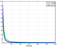
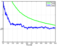
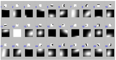
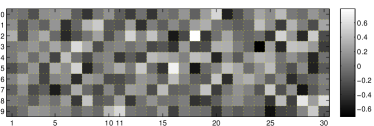
ShareBoost selects a subset of the templates $j_{1},\ldots,j_{T}$ where each $j_{i}$ represents some template pair $(w_{f_{i}},g_{f_{i}}^{c_{i}})$, and the matrix $W\in R^{k\times T}$. A test image $I$ is then converted to $\tilde{\mathbf{x}}\in R^{T}$ using $\tilde{x}_{i}=\max\{(I\otimes w_{f_{i}})\times g_{f_{i}}^{c_{i}}\}$ with the maximum going over the image locations. The prediction $\hat{y}$ is then $\operatorname*{argmax}_{y\in[k]}(W\tilde{\mathbf{x}})_{y}$. Fig. 5(a) shows the first 30 templates that were chosen by ShareBoost and their corresponding spatial masks. For example, the first templates matches a digit part along the top of the image, the eleventh template matches a horizontal stroke near the top of the image and so forth. Fig. 5(b) shows the weights (columns of $W$) of the first 30 templates of the model that produced the best results. For example, the eleventh template which encodes a horizontal line close to the top is expected in the digit “9” but not in the digit “4”. Fig. 6 shows the 47 misclassified samples after $T=305$ rounds of ShareBoost, and Fig. 4 displays the convergence curve of error-rate as a function of the number of rounds.

In terms of run-time on a test image, the system requires $305$ convolutions of $7\times 7$ templates and $540$ dot-product operations which totals to roughly $3.3\cdot 10^{6}$ MAC operations — compared to around $7.5\cdot 10^{6}$ MAC operations of the top MNIST performer. Moreover, due to the fast convergence of ShareBoost, 75 rounds are enough for achieving less than $1\%$ error. Further improvements of ShareBoost on the MNIST dataset are possible such as by extending further the training set using more deformations and by increasing the pool of features with other type of descriptors – but those were not pursued here. The point we desired to make is that ShareBoost can achieve competitive performance with the top MNIST performers, both in accuracy and in run-time, with little effort in feature space design while exhibiting great efficiency during training time as well.

Figure 4: Convergence of Shareboost on the MNIST dataset as it reaches 47 errors. The set was expanded with 5 deformed versions of each input, using the method in [31]. Since the deformations are fairly strong, the training error is higher than the test. Zoomed in version shown on the right.

(a) Leading 30 selected features	(b) Corresponding columns of $W$

Figure 5: (a) The first 30 selected features for the MNIST dataset. Each feature is composed of a 7$\times$7 template and a position mask. (b) The corresponding columns of $W$. The entries of a column represents the ”sharing” among classes pattern. For example, the eleventh template which encodes a horizontal line close to the top is expected in the digits “9,8,5” but not in digit “4”.

Figure 6: ShareBoost achieves an error of $0.47\%$ on the test set which translates to $47$ mistakes displayed above. Each error test example is displayed together with its predicted and True labels.

7.5 Comparing ShareBoost to kernel-based SVM

In the experiments on the MNIST data set reported above, each feature is the maximal response of the convolution of a $7\times 7$ patch over the image, weighted by a spatial mask.

One might wonder if the stellar performance of ShareBoost is maybe due to the patch-based features we designed. In this section we remove doubt by using ShareBoost for training a piece-wise linear predictor, as described in Section 4.2, on MNIST using generic features. We show that ShareBoost comes close to the error rate of SVM with Gaussian kernels, while only requiring $230$ anchor points, which is well below the number of support-vectors needed by kernel-SVM. This underscores the point that ShareBoost can find an extremely fast predictor without sacrificing state-of-the-art performance level.

Figure 7: Test accuracy of ShareBoost on the MNIST dataset as a function of the number of rounds using the generic piece-wise linear construction. Blue: train accuracy. Red: test accuracy. Dashed: SVM with Gaussian kernel accuracy.

Recall that the piece-wise linear predictor is of the following form:

$$h({\mathbf{x}})=\operatorname*{argmax}_{y\in\mathcal{Y}}\left(\sum_{j\in{\cal I}}\boldsymbol{1}\!\left[\|{\mathbf{x}}-{\mathbf{v}}^{(j)}\|<r^{(j)}\right]\,(W_{y,\cdot}^{(j)}{\mathbf{x}}+b_{y}^{(j)})\right),$$

where ${\mathbf{v}}^{(j)}\in\mathbb{R}^{d}$ are anchor points with radius of influence $r^{(j)}$, and $W^{(j)},b^{(j)}$ define together a linear classifier for the $j$’th anchor. ShareBoost selects the set of anchor points and their radiuses together with the corresponding linear classifiers. In this context it is worthwhile to compare classification performance to SVM with Gaussian kernels applied in a 1-vs-all framework. Kernel-SVM also selects a subset of the training set $S$ with corresponding weight coefficients, thus from a mechanistic point of view our piece-wise linear predictor shares the same principles as kernel-SVM.

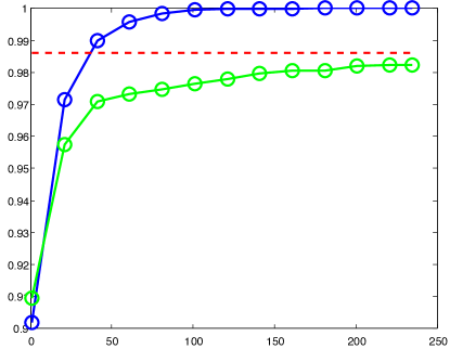
We performed a standard dimensionality reduction using PCA from the original raw pixel dimension of $28^{2}$ to $50$, i.e., every digit was mapped to ${\mathbf{x}}\in R^{50}$ using PCA. The pool of anchor points was taken from a reduced training set by means of clustering $S$ into 1500 clusters and the range of radius values per anchor point was taken from a discrete set of 35 values. Taken together, each round of ShareBoost selected an anchor point ${\mathbf{v}}^{(j)}$ and radius $r^{(j)}$ from a search space of size $52500$. Fig. 7 shows the error-rate per ShareBoost rounds. As can be seen, ShareBoost comes close to the error rate of SVM while only requiring $230$ anchor points, which is well below the number of support-vectors needed by kernel-SVM. This underscores the point that ShareBoost can find an extremely fast predictor without sacrificing state-of-the-art performance level.

8 Acknowledgements

We would like to thank Itay Erlich and Zohar Bar-Yehuda for their dedicated contribution to the implementation of ShareBoost.

Appendix A Proofs

A.1 Proof of Theorem 1

The proof is based on an analysis of the Natarajan dimension of the class of matrices with small number of non-zero columns. The Natarajan dimension is a generalization of the VC dimension for classes of multiclass hypotheses. In particular, we rely on the analysis given in Theorem 25 and Equation 6 of [9]. This implies that if the set of $T$ columns of $W$ are chosen in advance then

$$\operatorname*{\mathbb{P}}_{({\mathbf{x}},y)\sim\mathcal{D}} \left[h_{W}({\mathbf{x}})\neq y\right]~{}\leq~{}\operatorname*{\mathbb{P}}_{({\mathbf{x}},y)\sim S}\left[h_{W}({\mathbf{x}})\neq y\right]+O\left(\sqrt{Tk\log(Tk)\log(k)+\log(1/\delta)}/\sqrt{|S|}\right)~{}.$$

Applying the union bound over all $T\choose d$ options to choose the relevant features we conclude our proof.

A.2 Proof of Theorem 2

To prove the theorem, we start by establishing a certain smoothness property of $L$. First, we need the following.

Lemma 1

. Let $\ell:\mathbb{R}^{k}\to\mathbb{R}$ be defined as

$$\ell({\mathbf{v}})=\log\left(1+\sum_{i\in[k]\setminus\{j\}}e^{1-v_{j}+v_{i}}\right)~{}.$$

Then, for any ${\mathbf{u}},{\mathbf{v}}$ we have

$$\ell({\mathbf{u}}+{\mathbf{v}})\leq\ell({\mathbf{u}})+\langle\nabla\ell({\mathbf{u}}),{\mathbf{v}}\rangle+\|{\mathbf{v}}\|_{\infty}^{2}~{}.$$

Proof  Using Taylor’s theorem, it suffices to show that the Hessian of $\ell$ at any point satisfies

$${\mathbf{v}}^{\dagger}H{\mathbf{v}}\leq 2\|{\mathbf{v}}\|_{\infty}^{2}~{}.$$

Consider some vector ${\mathbf{w}}$ and without loss of generality assume that $j=1$. We have,

$$\frac{\partial\ell({\mathbf{w}})}{\partial w_{1}}=-\frac{\sum_{i=2}^{k}e^{1-w_{1}+w_{i}}}{1+\sum_{p=2}^{k}e^{1-w_{1}+w_{p}}}\stackrel{{\scriptstyle\mathrm{def}}}{{=}}\alpha_{1}$$

and for $i\geq 2$

$$\frac{\partial\ell({\mathbf{w}})}{\partial w_{i}}=\frac{e^{1-w_{1}+w_{i}}}{1+\sum_{p=2}^{k}e^{1-w_{1}+w_{p}}}\stackrel{{\scriptstyle\mathrm{def}}}{{=}}\alpha_{i}~{}.$$

Note that $-\alpha_{1}=\sum_{i=2}^{k}\alpha_{1}\leq 1$, and that for $i\geq 2$, $\alpha_{i}\geq 0$. Let $H$ be the Hessian of $\ell$ at ${\mathbf{w}}$. It follows that for $i\geq 2$,

$$H_{i,i}=\frac{e^{1-w_{1}+w_{i}}}{1+\sum_{p=2}^{k}e^{1-w_{1}+w_{i}}}-\frac{(e^{1-w_{1}+w_{i}})^{2}}{1+(\sum_{p=2}^{k}e^{1-w_{1}+w_{i}})^{2}}=\alpha_{i}-\alpha_{i}^{2}~{}.$$

In addition, for $j\neq i$ where both $j$ and $i$ are not $1$ we have

$$H_{i,j}=\frac{0-e^{1-w_{1}+w_{i}}e^{1-w_{1}+w_{j}}}{(\sum_{p=2}^{k}e^{1-w_{1}+w_{i}})^{2}}=-\alpha_{i}\alpha_{j}~{}.$$

For $i=1$ we have

$$H_{1,1}=-\alpha_{1}-\alpha_{1}^{2}$$

and for $i>1$

$$H_{i,1}=-\alpha_{i}-\alpha_{1}\alpha_{i}$$

We can therefore rewrite $H$ as

$$H = -\alpha\alpha^{\dagger}+\textrm{diag}([-\alpha_{1},\alpha_{2},\ldots,\alpha_{k}])-{\mathbf{e}}_{1}[0,\alpha_{1},\ldots,\alpha_{k}]$$

$$-[0,\alpha_{1},\ldots,\alpha_{k}]^{\dagger}({\mathbf{e}}_{1})^{\dagger}~{}.$$

It thus follows that:

$${\mathbf{v}}^{\dagger}H{\mathbf{v}} =-(\langle\alpha,{\mathbf{v}}\rangle)^{2}-\alpha_{1}v_{1}^{2}+\sum_{i>1}\alpha_{i}v_{i}^{2}-2v_{1}\sum_{i>1}\alpha_{i}v_{i}$$

$$\leq 0+\sum_{i>1}\alpha_{i}(v_{i}^{2}-v_{1}^{2}-2v_{1}v_{i})$$

$$=\sum_{i>1}\alpha_{i}((v_{i}-v_{1})^{2}-2v_{1}^{2})$$

$$\leq 2\max_{i}{\mathbf{v}}_{i}^{2}=2\|{\mathbf{v}}\|_{\infty}^{2}~{},$$

where the last step is because for any $v_{i}\in[-c,c]$, the function $f(v_{1})=(v_{i}-v_{1})^{2}-2v_{1}^{2}$ receives its maximum when $v_{1}=-v_{i}$ and then its value is $2v_{i}^{2}$. This concludes our proof.  

The above lemma implies that $L$ is smooth in the following sense:

Lemma 2

For any $W,U$ s.t. $U={\mathbf{u}}\,{\mathbf{e}}_{r}^{\dagger}$ (that is, only the $r$’th column of $U$ is not zero) we have that

$$L(W-U)\leq L(W)-\langle\nabla L(W),U\rangle+\|{\mathbf{u}}\|_{\infty}^{2}~{}.$$

Proof  Recall that $L(W)$ is the average over $({\mathbf{x}},y)$ of a function of the form $\ell(W{\mathbf{x}})$, where $\ell$ is as defined in Lemma 1. Therefore,

$$\ell((W+U){\mathbf{x}}) \leq\ell(W{\mathbf{x}})+\langle\nabla\ell(W{\mathbf{x}}),U{\mathbf{x}}\rangle+\|U{\mathbf{x}}\|_{\infty}^{2}$$

$$=\ell(W{\mathbf{x}})+\langle\nabla\ell(W{\mathbf{x}}),U{\mathbf{x}}\rangle+|x_{r}|^{2}\|{\mathbf{u}}\|_{\infty}^{2}$$

$$\leq\ell(W{\mathbf{x}})+\langle\nabla\ell(W{\mathbf{x}}),U{\mathbf{x}}\rangle+\|{\mathbf{u}}\|_{\infty}^{2}~{},$$

where the last inequality is because we assume that $\|{\mathbf{x}}\|_{\infty}\leq 1$ for all ${\mathbf{x}}$. The above implies that

$$L(W-U)\leq L(W)-\langle\nabla L(W),U\rangle+\|{\mathbf{u}}\|_{\infty}^{2}~{}.$$ (8)

 

Equipped with the smoothness property of $L$, we now turn to show that if the greedy algorithm has not yet identified all the features of $W^{\star}$ then a single greedy iteration yields a substantial progress. We use the notation ${\mathrm{supp}}(W)$ to denote the indices of columns of $W$ which are not all-zeros.

Lemma 3

Let $F,\bar{F}$ be two subsets of $[d]$ such that $\bar{F}-F\neq\emptyset$ and let

$$W=\operatorname*{argmin}_{V:{\mathrm{supp}}(V)=F}L(V)~{}~{}~{}~{},~{}~{}~{}~{}W^{\star}=\operatorname*{argmin}_{V:{\mathrm{supp}}(V)=\bar{F}}L(V)~{}~{}.$$

Then, if $L(W)>L(W^{\star})$ we have

$$L(W)-\min_{{\mathbf{u}}}L(W+{\mathbf{u}}{\mathbf{e}}_{j}^{\dagger})~{}\geq~{}\frac{\left(L(W)-L(W^{\star})\right)^{2}}{4\,\left(\sum_{i\in\bar{F}-F}\|W^{\star}_{\cdot,i}\|_{\infty}\right)^{2}},$$

where $j=\operatorname*{argmax}_{i}\|\nabla_{i}L(W)\|_{1}$.

Proof  To simplify notation, denote $F^{c}=\bar{F}-F$. Using Lemma 2 we know that for any ${\mathbf{u}}$:

$$L(W-{\mathbf{u}}{\mathbf{e}}_{j}^{\dagger})\leq L(W)-\langle\nabla L(W),{\mathbf{u}}{\mathbf{e}}_{j}^{\dagger}\rangle+\|{\mathbf{u}}\|_{\infty}^{2}~{},$$

In particular, the above holds for the vector of ${\mathbf{u}}=\tfrac{1}{2}\|\nabla_{j}L(W)\|_{1}\,{\mathrm{sgn}}(\nabla_{j}L(W))$ and by rearranging we obtain that

$$L(W)-L(W-{\mathbf{u}}{\mathbf{e}}_{j}^{\dagger}) \geq\langle\nabla L(W),{\mathbf{u}}{\mathbf{e}}_{j}^{\dagger}\rangle-\|{\mathbf{u}}\|_{\infty}^{2}$$

$$=\tfrac{1}{4}\|\nabla_{j}L(W)\|_{1}^{2}~{}.$$

It is therefore suffices to show that

$$\frac{1}{4}\|\nabla_{j}L(W)\|_{1}^{2}~{}\geq~{}\frac{\left(L(W)-L(W^{\star})\right)^{2}}{4\left(\sum_{i\in\bar{F}-F}\|W^{\star}_{\cdot,i}\|_{\infty}\right)^{2}}~{}.$$

Denote $s=\sum_{j\in F^{c}}\|W^{\star}_{\cdot,j}\|_{\infty}$, then an equivalent inequality is

$$s\,\|\nabla_{j}L(W)\|_{1}~{}\geq~{}L(W)-L(W^{\star})~{}.$$

From the convexity of $L$, the right-hand side of the above is upper bounded by $\langle\nabla L(W),W-W^{\star}\rangle$. Hence, it is left to show that

$$s\,\|\nabla_{j}L(W)\|_{1}~{}\geq~{}\langle\nabla L(W),W-W^{\star}\rangle~{}.$$

Since we assume that $W$ is optimal over $F$ we get that $\nabla_{i}L(W)=\mathbf{0}$ for all $i\in F$, hence $\langle\nabla L(W),W\rangle=0$. Additionally, $W^{\star}_{\cdot,i}=\mathbf{0}$ for $i\not\in\bar{F}$. Therefore,

$$\langle\nabla L(W),W-W^{\star}\rangle =-\sum_{i\in F^{c}}\langle\nabla_{i}L(W),W^{\star}_{\cdot,i}\rangle$$

$$\leq\sum_{i\in F^{c}}\|\nabla_{i}L(W)\|_{1}\,\|W^{\star}_{\cdot,i}\|_{\infty}$$

$$\leq s\,\max_{i}\|\nabla_{i}L(W)\|_{1}$$

$$=s\,\|\nabla_{j}L(W)\|_{1}~{},$$

and this concludes our proof.  

Using the above lemma, the proof of our main theorem easily follows.

Proof [of Theorem 2] Denote $\epsilon_{t}=L(W^{(t)})-L(W^{\star})$, where $W^{(t)}$ is the value of $W$ at iteration $t$. The definition of the update implies that $L(W^{(t+1)})\leq\min_{i,{\mathbf{u}}}\,L(W^{(t)}+{\mathbf{u}}{\mathbf{e}}_{i}^{\dagger})$. The conditions of Lemma 3 hold and therefore we obtain that (with $F=F^{(t)}$)

$$\begin{split}\epsilon_{t}-\epsilon_{t+1}&=L(W^{(t)})-L(W^{(t+1)})\geq~{}\frac{\epsilon_{t}^{2}}{4\,\left(\sum_{i\in\bar{F}-F}\|W^{\star}_{\cdot,i}\|_{\infty}\right)^{2}}\\ &\geq~{}\frac{\epsilon_{t}^{2}}{4\,\|W^{\star}\|_{\infty,1}^{2}}~{}.\end{split}$$ (9)

Using Lemma B.2 from [30], the above implies that for $t\geq 4\,\|W^{\star}\|_{\infty,1}^{2}/\epsilon$ we have that $\epsilon_{t}\leq\epsilon$, which concludes our proof.

References

- Amit et al. [2007] Amit, Y., Fink, M., Srebro, N., and Ullman, S. Uncovering shared structures in multiclass classification. In International Conference on Machine Learning, 2007.
- Argyriou et al. [2006] Argyriou, A., Evgeniou, T., and Pontil, M. Multi-task feature learning. In NIPS, pp. 41–48, 2006.
- Bach [2008] Bach, F.R. Consistency of the group lasso and multiple kernel learning. J. of Machine Learning Research, 9:1179–1225, 2008.
- Belongie et al. [2002] Belongie, S., Malik, J., and Puzicha, J. Shape matching and object recognition using shape contexts. IEEE PAMI, 24(4):509–522, April 2002.
- Bengio et al. [2011] Bengio, S., Weston, J., and Grangier, D. Label embedding trees for large multi-class tasks. In NIPS, 2011.
- Candes & Tao [2005] Candes, E.J. and Tao, T. Decoding by linear programming. IEEE Trans. on Information Theory, 51:4203–4215, 2005.
- Ciresan et al. [2010] Ciresan, D. C., Meier, U., G., L. Maria, and Schmidhuber, J. Deep big simple neural nets excel on handwritten digit recognition. CoRR, 2010.
- Crammer & Singer [2003] Crammer, K. and Singer, Y. Ultraconservative online algorithms for multiclass problems. Journal of Machine Learning Research, 3:951–991, 2003.
- Daniely et al. [2011] Daniely, A., Sabato, S., Ben-David, S., and Shalev-Shwartz, S. Multiclass learnability and the erm principle. In COLT, 2011.
- Davis et al. [1997] Davis, G., Mallat, S., and Avellaneda, M. Greedy adaptive approximation. Journal of Constructive Approximation, 13:57–98, 1997.
- Decoste & Bernhard [2002] Decoste, D. and Bernhard, S. Training invariant support vector machines. Mach. Learn., 46:161–190, 2002.
- Donoho [2006] Donoho, D.L. Compressed sensing. In Technical Report, Stanford University, 2006.
- Duchi & Singer [2009] Duchi, J. and Singer, Y. Boosting with structural sparsity. In Proc. ICML, pp. 297–304, 2009.
- Duda & Hart [1973] Duda, R. O. and Hart, P. E. Pattern Classification and Scene Analysis. Wiley, 1973.
- Fink et al. [2006] Fink, M., Shalev-Shwartz, S., Singer, Y., and Ullman, S. Online multiclass learning by interclass hypothesis sharing. In International Conference on Machine Learning, 2006.
- Freund & Schapire [1999] Freund, Y. and Schapire, R. E. A short introduction to boosting. J. of Japanese Society for AI, pp. 771–780, 1999.
- Freund & Schapire [1997] Freund, Y. and Schapire, R.E. A decision-theoretic generalization of on-line learning and an application to boosting. Journal of Computer and System Sciences, pp. 119–139, 1997.
- Hastie & Tibshirani [1995] Hastie, T.J. and Tibshirani, R.J. Generalized additive models. Chapman & Hall, 1995.
- Hsu et al. [2010] Hsu, D., Kakade, S.M., Langford, J., and Zhang, T. Multi-label prediction via compressed sensing. In NIPS, 2010.
- Huang & Zhang [2010] Huang, J. and Zhang, T. The benefit of group sparsity. Annals of Statistics, 38(4), 2010.
- Huang et al. [2009] Huang, J., Zhang, T., and Metaxas, D.N. Learning with structured sparsity. In ICML, 2009.
- Lanckriet et al. [2004] Lanckriet, G.R.G., Cristianini, N., Bartlett, P.L., Ghaoui, L. El, and Jordan, M.I. Learning the kernel matrix with semidefinite programming. J. of Machine Learning Research, pp. 27–72, 2004.
- LeCun et al. [1998] LeCun, Y. L., Bottou, L., Bengio, Y., and Haffner, P. Gradient-based learning applied to document recognition. Proceedings of IEEE, pp. 2278–2324, 1998.
- Majumdar & Ward [2009] Majumdar, A. and Ward, R.K. Fast group sparse classification. Electrical and Computer Engineering, Canadian Journal of, 34(4):136–144, 2009.
- Natarajan [1995] Natarajan, B. Sparse approximate solutions to linear systems. SIAM J. Computing, pp. 227–234, 1995.
- Nesterov & Nesterov [2004] Nesterov, Y. and Nesterov, I.U.E. Introductory lectures on convex optimization: A basic course, volume 87. Springer Netherlands, 2004.
- Quattoni et al. [2008] Quattoni, A., Collins, M., and Darrell, T. Transfer learning for image classification with sparse prototype representations. In CVPR, 2008.
- Quattoni et al. [2009] Quattoni, A., Carreras, X., Collins, M., and Darrell, T. An efficient projection for l 1,infinity regularization. In ICML, pp. 108, 2009.
- Schapire & Singer [1999] Schapire, R. E. and Singer, Y. Improved boosting algorithms using confidence-rated predictions. Machine Learning, 37(3):1–40, 1999.
- Shalev-Shwartz et al. [2010] Shalev-Shwartz, S., Zhang, T., and Srebro, N. Trading accuracy for sparsity in optimization problems with sparsity constraints. Siam Journal on Optimization, 20:2807–2832, 2010.
- Simard et al. [2003] Simard, P. Y., S., Dave, and Platt, John C. Best practices for convolutional neural networks applied to visual document analysis. Document Analysis and Recognition, 2003.
- Taskar et al. [2003] Taskar, B., Guestrin, C., and Koller, D. Max-margin markov networks. In NIPS, 2003.
- Thrun [1996] Thrun, S. Learning to learn: Introduction. Kluwer Academic Publishers, 1996.
- Tibshirani [1996] Tibshirani, R. Regression shrinkage and selection via the lasso. J. Royal. Statist. Soc B., 58(1):267–288, 1996.
- Torralba et al. [2007] Torralba, A., Murphy, K. P., and Freeman, W. T. Sharing visual features for multiclass and multiview object detection. IEEE Transactions on Pattern Analysis and Machine Intelligence (PAMI), pp. 854–869, 2007.
- Tropp & Gilbert [2007] Tropp, J.A. and Gilbert, A.C. Signal recovery from random measurements via orthogonal matching pursuit. Information Theory, IEEE Transactions on, 53(12):4655–4666, 2007.
- Turlach et al. [2000] Turlach, B. A, V., W. N, and Wright, Stephen J. Simultaneous variable selection. Technometrics, 47, 2000.
- Vapnik [1998] Vapnik, V. N. Statistical Learning Theory. Wiley, 1998.
- Xing et al. [2003] Xing, E., Ng, A.Y., Jordan, M., and Russell, S. Distance metric learning, with application to clustering with side-information. In NIPS, 2003.
- Zhang [2004] Zhang, T. Class-size independent generalization analysis of some discriminative multi-category classification. In NIPS, 2004.
- Zhou et al. [2010] Zhou, X., Yu, K., Zhang, T., and Huang, T. Image classification using super-vector coding of local image descriptors. Computer Vision–ECCV 2010, pp. 141–154, 2010.