Stochastic (in)stability of synchronisation of oscillators on networks
Abstract
We consider the influence of correlated noise on the stability of synchronisation of oscillators on a general network using the Kuramoto model for coupled phases . Near the fixed point the impact of the noise is analysed through the Fokker-Planck equation. We deem the stochastic system to be ‘weakly unstable’ if the Mean First Passage Time for the system to drift outside the fixed point basin of attraction is less than the time for which the noise is sustained. We argue that a Mean First Passage Time, computed near the phase synchronised fixed point, gives a useful lower bound on the tolerance of the system to noise. Applying the saddle point approximation, we analytically derive general thresholds for the noise parameters for weak stochastic stability. We illustrate this by numerically solving the full Kuramoto model in the presence of noise for an example complex network.
keywords:
synchronisation oscillator Kuramoto noise Fokker-Planck mean first passage timeMSC:
[2010] 33D50 34F051 Introduction
The spontaneous generation of ordered or patterned behaviour is a significant property of dynamical systems of many nonlinearly coupled heterogeneous entities. This behaviour is relevant to a vast array of real world systems: physical, chemical, biological, ecological and social. Where the dynamics of the component level entities have cyclic characteristics, the model of coupled phase oscillators on a network is a compact mathematical representation offering much insight. The Kuramoto model [1] is a simple example of this, exhibiting transition from incoherence to phase synchrony as a single coupling constant is varied from small to large values. In this paper we explore how thresholds for the strength of noise applied for a finite period of time to the system close to the synchronised state can be determined such that stability is maintained.
The Kuramoto model [1, 2] involves one-dimensional phase oscillators described by angles coupled on a network described by an undirected graph of size . The model is given by the first order differential equation,
| (1) |
Here is the adjacency matrix encoding the graph structure, are intrinsic frequencies of the oscillators, usually drawn from some statistical distribution, and is a global coupling controlling the strength of mutual adjustment between adjacent oscillators. At zero coupling the system behaves incoherently. Increasing the coupling drives the bulk of oscillators to lock into a single core that undergoes harmonic motion according to the average of the frequencies, while others undergo random motion about the unit circle. At lower coupling values phase velocities can synchronise, , and at stronger coupling the phases themselves synchronise, . We are interested in the regime where the latter applies to all nodes, and will refer to this as ‘phase synchronisation’. Kuramoto [1] considered the complete () infinite () case, which can be solved by fluid dynamics techniques. Stability and noise have been separately studied with such methods in [3, 4]. Unfortunately, these cannot be generalised to non-complete finite graphs, in which we are interested. Similarly, it is difficult to draw general conclusions from numerical studies of specific graphs such as [5].
Noise is invoked either because the fine-structure of component entities cannot be fully encoded in deterministic equations such as Eq.(1), or to undermine/encourage known deterministic behaviours. One is interested then in the threshold for tolerance to noise either to understand the limitations of a deterministic model of a system or the capacity of the known deterministic system to cope with imposed noise. In [6], Sakaguchi applied stochastic flucuations to the intrinsic frequencies in Eq.(1) and obtained an equivalent result to Kuramoto in [1] in the complete infinite case. Park, Kim and Ryu [7, 8] have numerically examined noise in the equal frequencies and complete network Kuramoto model (using an extra ‘pinning term’) but, again, their insights cannot be generalised. Analytic approaches to deterministic (Lyapunov) stability of synchronisation, such as that of Pecora and Carroll [9], are welcoming because they open the door to analysis of general graphs and frequencies. The non-polynomial interactions in Eq.(1) mean that the method of [9] only works close to phase synchrony [10]. Noise can nevertheless be examined in the neighborhood of the fixed point basin of attraction. It is known that, except for special cases of stochastic systems that are ‘classically stable’ [11], noise leads to drift outside some bounded region if an arbitrary amount of time is permitted. However, for many biological and social systems, the finite life of entities mean that noise need/may not be sustained indefinitely. There is value then in a criterion for ‘weak stochastic stability’ for the Kuramoto model, so that stability of phase synchronisation can be guaranteed within a finite period of application of noise.
We emphasise that Eq.(1) combined with noise is a stochastic generalisation of the Kuramoto model. Noise can be injected through a combination of fluctuations on the coupling, the frequencies, and the network topology. It is known that near phase synchrony a certain decoupling of the dynamics into collective modes occurs [10, 12]. We therefore adopt the strategy of applying noise to these collective modes. We solve for the stationary probability distributions for these modes from the Fokker-Planck equation. By then computing the Mean First Passage Time (MFPT) for the modes to cross an effective boundary of the basin of attraction for the phase synchronised fixed point we may analytically derive thresholds for various parameters, thereby guaranteeing weak stochastic stability.
By basing ourselves in an approximation near the phase synchronised fixed point, our results do not include effects of recoupling by the modes as noise pushes them outside their basin of attraction, which in turn can lead to quite exotic stabilising effects in the presence of noise. This makes our analytical determination of a Mean First Passage Time a strong under-estimate of the full non-linear result. However, this provides a useful lower bound on tolerances of the system to noise-driven instability. This result enables thresholds to noise to be computed for general graphs and frequencies. The focus of our paper is what can be computed analytically, however we illustrate our results - including the nonlinear effects our analytic approach omits - by numerically solving the full Kuramoto system for a specific non-trivial graph.
We formulate the model in the next section, and then discuss our solution method for the Fokker-Planck system; we show here an example complete numerical solution exhibiting noise generated instability. We next state the results for the stationary probability distribution functions in preparation for characterising the stochastic stability in terms of the MFPT and show how general stability thresholds in the noise parameters can be derived. Subsequently, with a numerical solution of the full model we illustrate how, using the MFPT computed near phase synchrony, stochastic instability can be avoided. We discuss implications of our results for general graphs and look ahead to future work. Details of some derivations are relegated to three appendices.
2 Stochastic equations close to synchrony
2.1 Laplacian decomposition of deterministic case
As mentioned in the introduction, close to phase synchrony the dynamics decouples into independent behaviours of certain collective modes [10, 12]. This decoupling is based on a decomposition of the network into eigenvectors of the graph Laplacian. For a connected unweighted undirected graph the Laplacian is defined as [13]
| (2) |
with the degree of node . The spectrum of Laplacian eigenvalues is positive semi-definite, as explained by Bollobás in [13]. The corresponding system of orthonormal eigenvectors satisfy
Most immediately useful here is the property that the lowest eigenvalue vanishes, . For a connected graph the first non-zero eigenvalue is known as the algebraic connectivity [14]. Graphs with are easily disconnected by removal of a small number of links.
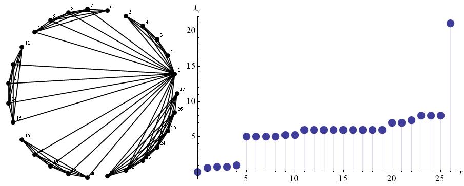
An example of a connected graph of nodes, a variation of a graph due to Ravasz and Barabási (RB) [15], and its related Laplacian spectrum are shown in Fig.1; we shall later use this ‘RB’ graph to illustrate the properties we derive in this paper. In particular, we observe in the spectrum of Fig.1 the single zero eigenvalue, a sequence of four eigenvalues less than one, a broad set between values five and ten, and then the jump at with . That there are four eigenvalues less than one, close to , is indicative of the hierarchy and symmetry of the graph; the circular embedding in Fig.1 reveals a number of ways of disconnecting the graph with four link removals. The proportions of eigenvalues less than one and, respectively, greater than one will vary for graphs of different classes.
In considering how noise can be applied to a network in this context, it is important to explain the network interpretation of the Laplacian eigenvectors . They represent ‘weighted’ sub-graphs of : the component is the (not necessarily positive) numerical weight with which a node is represented in the r-th sub-graph. For the RB graph in Fig.1, for example, the eigenvector corresponding to the third eigenvalue is shown, alongside the eigenvectors for , in Fig.2. Thus describes a subgraph consisting of the nodes with both positive and negative weights applied. We may further say that within the sub-graph, the nodes and form finer sub-structures that are internally correlated but anti-correlated with respect to each other. Such sub-graphs are the network analogue of the combinations of atomic bonds that give rise to phonons as collective excitations in crystal lattices.
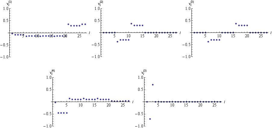
In Fig.2 we observe quite different characteristics in the structures of the lowest lying eigenvectors in terms of the proportion of positive, negative and zero values.
The Laplacian is, in fact, a Laplace-Beltrami operator on the manifold described by . To this extent it reflects properties well-known in condensed matter systems: the eigenvalues are a ‘momentum-squared’ and their corresponding eigenvectors act like ‘probes’ on the sub-graphs. The eigenvectors corresponding to low-lying eigenvalues involve larger scale sub-graphs of while those for higher values reflect finer structures in the graph. This ‘probing’ of sub-structures will vary according to the precision with which one may quantify or manipulate properties of nodes of the network. If the network represents a set of physical or chemical entities one may have a considerably precise means of measuring or altering properties of the nodes. For example, in the case of condensed matter systems one is typically able to excite individual frequency modes of phonons. Contrastingly, if the network is a biological or social system the means of measuring or manipulating the properties may be more limited. Either way, it is important that the probing of sets of nodes may be distinguished in relative strength and in sign, that it may be applied positively or negatively at different parts of the network according to the structure of an eigenvector. We discuss this further below in the context of applying noise.
We now expand the phase angles of the Kuramoto model in the Laplacian basis of eigenmodes,
| (3) |
We refer to the as the Laplacian ‘modes’ of the Kuramoto system. Treating as the components to an -dimensional vector, , with the average over the frequency distribution, we can form the scalar product of the frequency vector and the Laplacian eigenvectors
We now consider the system close to a point of phase synchronisation (),
| (4) |
where from this point we summarise the coupling as . Inserting the decomposition Eq.(3) into the truncated equation of motion Eq.(4), we can extract equations for the eigenmodes ,
| (5) |
while the zero mode of Eq.(4) gives at time after initial time . We see that, indeed, to this order, the modes are decoupled. The exact solution to Eq.(5) is:
| (6) |
where represents the initial configuration. Taking the large limit of this shows that there is a fixed point
| (7) |
whose stability is determined by the Lyapunov exponents in Eq.(6). They do not change sign due to the semi-definiteness of the Laplacian spectrum [13]. Thus phase synchrony is stable in every direction of trajectory space [10] (whose axes can be labelled by the modes ): fluctuations on are small,
| (8) |
as long as the condition is true at the initial time , and
| (9) |
so that the approximations leading to Eq.(4) are valid over all times.
2.2 Bounding the basin of attraction
The define the origin of a basin of attraction in trajectory space whose curvature in every direction of the origin is concave since the are all positive. The boundary of the basin is determined by the range in which , with the difference between any two phases. This leads to . The quantity is the threshold difference in phases for which the linear approximation to sine is deemed valid. To convert this into a general boundary on is difficult.
Some authors have, effectively, derived bounds on norms over the modes [16, 17] in order to give the critical coupling in terms of some aggregate property of the frequency distribution - in the spirit of Kuramoto’s analytical result for the critical coupling of the complete graph [1].
Our experience with numerical solutions of systems with 20-30 nodes [10] is that is a sufficient indicator of the boundary. We shall see this also in the specific example of the RB graph we use in this work. In Appendix A we show, based on the structure of underlying Laplacian eigenvectors and the scaling of their components, how this heuristic choice of the boundary scales with the size of the graph . In the interests of brevity we simply state the basic result here.
For graphs where the lowest non-zero eigenvalue is of the order , , the graph is highly connected, close to a complete graph. The corresponding low-lying eigenvectors are then highly ‘localised’, namely have non-zero components focused in two nodes: for two values of . In that case, the boundary of the basin in can be taken as
| (10) |
At another extreme, a large graph which is easily disconnected into two nearly complete graph components of size by a few link removals, will have an eigenvector which will look like a step function, going from values to at the nodes that form the bridge between the two parts. In that case the boundary of the basin in scales with :
| (11) |
In between these two extremes are graphs whose sub-structures do not scale uniformly with : for example, reproducing the structure of the RB graph (which is designed to exhibit hierarchy and thus be scale-free) for larger . For these the simple scaling arguments we give in Appendix A do not work. Given that at the extremes the size of the basin in increases, it follows that maintaining a heuristic boundary at is an under-estimate. Since we are looking for thresholds for stability under noise, it is reasonable we remain with this choice in the following.
The independence of Laplacian modes, which survives considerably far from the regime where the ‘smallness’ criterion of Eqs.(8) and (9) applies [12], leads to the following simple intuitive picture. The Laplacian eigenmodes with largest values of indicate whether the system can phase synchronise. This quantity brings together the three key elements of the deterministic system: the frequencies, the network topology (through the Laplacian eigenvalues and eigenvectors) and the coupling constant. There are a number of ways the elements may combine to satisfy Eq.(9): sufficiently strong coupling, sufficiently narrow frequency range, and sufficiently large , which amounts to sufficiently strong connectivity. Thus the mode most susceptible to disruption from synchronicity corresponds to that for which is closest to one, which is not necessarily that corresponding to .
We obtain from Eq.(9) a weak type of criterion for synchronisation [16], But because we cannot be more precise about the basin boundary we cannot, at this order, extract a sharp threshold of coupling which distinguishes synchrony from incoherence as distinct phases. Second order fluctuations offer some scope for overcoming this [10]. However, noise induced instabilities are our concern in this paper. Specifically, we shall pose the question: if the deterministic system is stable, according to Eq.(9), what parameter choices in the noise will render the stochastic system unstable?
2.3 Applying noise: Stochastic system in Laplacian decomposition
The well-known logistic equation for population dynamics can be brought to the form Eq.(5) after a change of variables. This is our clue for examining the system in the presence of stochastic fluctuations: we may exploit a significant body of work on noisy population dynamics. Specifically, in [18] and references therein, Goŕa considered a generalisation of the logistic equation by perturbation with two correlated Gaussian White Noise (GWN) terms, and ; the superscripts and stand for additive and multiplicative respectively.
We perform a similar analysis by letting the deterministic system reach a state close to synchrony (Eq.(4)). At time we apply a stochastic disturbance to the system for a finite period of time . We wish to apply noise both additively, on top of the static but otherwise random frequencies at each node, and multiplicatively - namely to the coupling strength of the links between each node. Hence for each graph node we apply the following additive weighted sum of random time dependent noises,
| (12) |
where the Heaviside step functions, , act to switch the noise on and off. Similarly, for each graph link we apply the following multiplicative weighted sum, , of random time dependent noises,
| (13) |
where .
For the full Kuramoto system, applying the noise Eqs.(12,13) leads to the following Langevin-like equations [19]:
| (14) |
in Eq.(14) represents introducing noise on the natural frequencies, , of each graph node, while represents noise on the interaction between nodes and . This form means that nodes for which may nonetheless have noise applied across them. For a non-complete graph there is no natural structure for applying noise multiplicatively other than the graph itself, via for all (as in [7, 8]). Our prescription is, therefore, more general than applying noise uniformly to the existing connections in the static graph given by . However, it is by no means the most general type of noise that could be applied since there are only degrees of freedom (the values of ) for possible entries in a general matrix . Depending on the instantiation of the network, specific non-factoriseable forms for may arise organically. The advantage of our form is that the Fokker-Planck equation is factoriseable, and therefore analytically tractable, permitting us to make some definite statements of the impact of noise on stability of the fixed point.
Note also that the multiplicative noise in Eq.(14) is linear in the phase , implying that for large phases the multiplicative noise will dominate over the bounded sine interaction. This is certainly quite strong, but ultimately we are only interested in the behaviour of the system in the vicinity of phase synchrony so that the dynamics beyond the loss of synchrony will not be studied in any detail. Near phase synchrony, therefore, the system can be expressed either in terms of the phase angles or eigenmodes:
| (15) | |||
| (16) |
The additive and multiplicative GWN terms are themselves given in terms of uncorrelated GWN functions and through
| (17) |
where the following expectation values encode the absence of correlation between and :
The quantity is the diffusion constant. (As approaches zero we obtain the usual deterministic results.) Hence and are correlated in the following way,
| (18) |
We refer to the constant as the correlation parameter as it provides an indication of the mutual correlation between the noises applied to the natural frequencies and link interactions.
2.4 Solving the Langevin equations
Since Eq.(16) is linear in we can apply standard techniques to obtain the solution
| (19) |
where
For short time solutions we can obtain the following approximation to Eq.(19),
| (20) |
where . Here means the expectation value of given condition . We see that the deterministic Lypunov behaviour, given through , picks up a stochastic contribution; see also [20].
2.5 Classical stochastic stability
In [11], stochastic stability is defined as the property that a stochastic system will remain in a neighborhood of a fixed point for all time. We can identify such a case of the near-synchronised Kuramoto model with the following parameter assignments: , , and . This gives the Langevin system
| (21) |
Following [11] for Eq.(21) (for more details refer to B) we find that with
| (22) |
the system indeed remains close to the fixed point for all time. Note that later, when we numerically solve Eq.(14), we shall see solutions that stay close to the fixed point for all time. These are due to interactions inaccessible to the approximation to first order in fluctuations. Thus Eq.(22) leads to stochastically stability within the bounds of first order fluctuations.
We refer to the requirement that the system stay in the vicinity of the fixed point for as classical stochastic stability, an unnecessarily restrictive condition for many real world systems with living entities. We instead adopt a more flexible definition of stochastic stability based on the Mean First Passage Time and the finite time for which the noise is applied and, contrastingly, refer to this as weak stochastic stability.
2.6 Numerical behaviour of full stochastic Kuramoto system
To give a feel for the complete dynamics, before we proceed with analytical solutions near phase synchrony, we show the behaviour based on numerical solutions at a value of the coupling where the deterministic system is known to phase synchronise. We use the RB network [15] in Fig.1 for which synchronisation properties of the deterministic system are known [10]. We also used in [10] a set of intrinsic frequencies drawn from a uniform distribution in the range , for example the set in Fig.3.
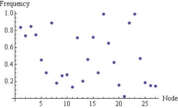
Then the largest values of the fixed point are . Note that both correspond to eigenvectors with all non-zero components. We therefore examine the mode, , because it involves fewer nodes with non-zero weights (as seen in Fig.2). The projection of the frequency vector onto this eigenvector is . We will use this mode and this frequency projection throughout the paper.
According to first order considerations of the deterministic system [10], for all couplings the system should be stably locked in a state of phase synchrony. Numerical calculations confirm this [10]. We therefore adopt a coupling , at which we know the deterministic system is phase synchronised, and examine the effect of noise on the Laplacian mode. Then . The initial configuration is also taken as . We numerically solve the system Eq.(14) using Mathematica for some 1000 instances, with noise as defined in Eqs.(12,13). In the presence of noise we generally find that points suffice up to time steps to manifest the key dynamics. At the system synchronises rapidly within a few time units. Thus guarantees the system is phase synchronised before the noise switches on. We choose
| (23) |
(Note that .)
At this point we temporarily use the traditional symbol for Kuramoto’s order parameter [1] (and no longer as a label for the Laplacian modes):
| (24) |
Values of reflect full phase synchrony, . At these settings, frequently the noise immediately causes the order parameter to deviate from but with a delay before the entire system of oscillators becomes chaotic.
At this stage, we set : the noise is sustained from the moment it begins to the end of the period over which we solve the system. We show in Fig.4 three instances of the typical behaviour. In one there is a delay between and between the initial impact of the noise and the eventual onset of chaos: steadily drops in value before oscillations begin. In another instance there is only a slight diminishing of and stabilisation at some state of partial synchronisation. In others the noise has had little impact over the period for which we solve the system.
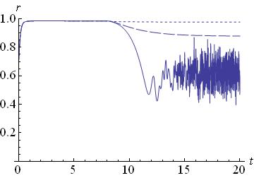
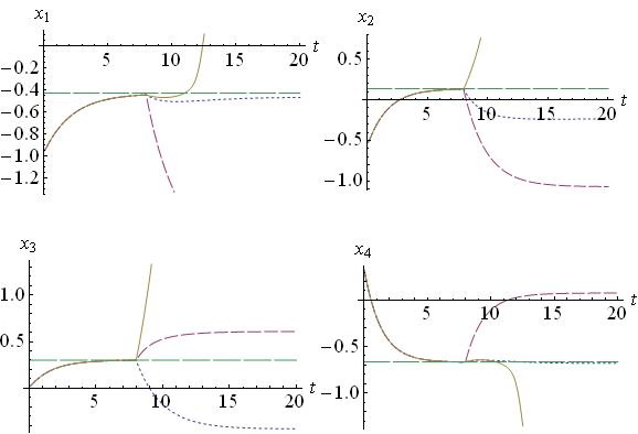
Examining the low-lying Laplacian modes we can understand this time delay in the instance where the order parameter becomes chaotic. The modes are plotted in Fig.5, where the fixed points for each are also indicated; the modes quickly settle to their fixed point before the noise is switched on. Because the eigenvectors all share common nodes with non-zero components there is an immediate effect at on all the modes, even though the noise has only been applied to the third Laplacian eigenvector. However after the noise is switched on each instance behaves quite differently. For the instance in Fig.4 in which the order parameter becomes chaotic - the solid line - we see that in Fig.5 all four of the lowest lying modes eventually diverge in positive or negative directions; again see the solid line in each case. Indeed, the period in which the order parameter decreases monotonically before showing oscillations coincides with the period in which the mode is approaching the value one (demonstrating that there is no ‘sharp’ threshold). Specifically, for this instance, we observe a difference in behaviour for the modes against : the latter two remain suppressed for some time before diverging, respectively, positively and negatively. This is consistent with the fact, visible in Fig.2, that the eigenvectors share common nodes of the same order of -0.5, while are somewhat suppressed at these nodes, but non-zero. However, clearly in Fig.5 the mode reaches the value one fastest, followed by , and then modes and turn around. We argue that this is evidence for driven to the edge of the basin of attraction first, followed closely by , but in the course of this non-linear interations switching on, driving and out of steady-state.
For the other instances, dotted and dashed lines in Fig.5, a type of stabilisation takes place in the presence of noise inside the original basin of attraction but not at the deterministic fixed point. This is evidently a consequence of competition between the deterministic and stochastic aspects of the system, about which our approach has little to say but warrants investigation in its own right. For the corresponding instances in Fig.4, the order parameter has stabilised to some near phase synchronisation value.
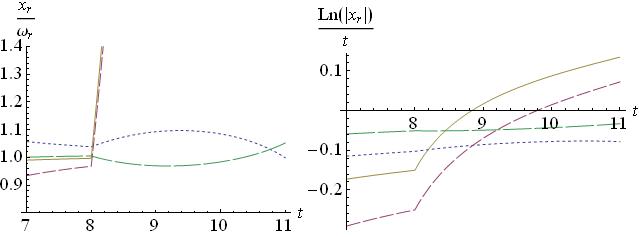
Selecting the particular instance where the order parameter in Fig.4 shows chaotic behaviour, and zooming in to the behaviour shortly after the noise is switched on we see in Fig.6 that the the deviation away from the fixed point is essentially linear consistent with the initial behaviour of an exponential. In the left hand plot of Fig.6, where we normalise by , we see that when and reach large values then and develop noticeable curvature. In the right hand plot for we see that the initial time dependence after the noise begins is consistent with exponential instability: the exponent is initially linear and has noise dependence, consistent with our solution to the Langevin equations, Eq.(20).
The curvature in and in Fig.6 coincides with and both of the order of one: they have left the effective basin of attraction. At this point the variations in the modes become nonlinear as a consequence of the restored interactions; it is at this point that the system has left the regime where our approximation Eq.(4) applies and the behaviour in Fig.4 is chaotic. We see that there is a regime in which the linearised system is valid. Our aim is to compute an average time over which this regime applies.
2.7 Fokker-Planck Equations
Rather than focusing on (where again labels the mode and not the Kuramoto order parameter) in the Langevin equations we address the probability density function for an ensemble of such . Denoted , it determines the probability that the random variable lies in the range . The Fokker-Planck equation governs the evolution of this probability density, given the system is initially in state at initial time :
where now represents the vector, in the Laplacian basis, of components . Because we shall always work in time periods where the noise is applied, we set the Heaviside functions to unity. From the Langevin equation Eq.(16) we follow Goŕa [18] (who uses the Itô interpretation) and derive the Fokker Planck equation [19],
| (25) |
where,
| (26) |
Here represents a diffusion matrix and a drift vector.
3 Solving the stationary Fokker-Planck equations and MFPT
3.1 Decoupling
As the diffusion matrix is diagonal, we decompose into a product of normal modes,
so that Eq.(25) decouples into separate equations for each
| (27) | |||||
Since we have decoupled the modes we herein drop the sub(super)scripts .
3.2 Stationary densities
As we shall see, the MFPT only relies on the stationary solution of the FP equation, so we shall not detail the time dependent solution to Eq.(25). Those interested in full time dependence are encouraged to refer to [21] and references therein. We solve for the stationary density of Eq.(27), denoted , by setting . We obtain the corresponding (Pearson’s) differential equation,
| (28) |
where the constant is chosen for convenience. is also referred to as a weight function.
There are three distinct forms of the stationary densities which are dependent on the following choices of :
-
1.
Case I, is constant;
-
2.
Case II, is quadratic with a single degenerate root; and
-
3.
Case III, is quadratic with non degenerate complex roots.
We now detail these individual cases.
3.2.1 Case I
For this case we set , hence only additive noise is present in the system. We rescale and shift to
in terms of which the normalised stationary probability density function is
| (29) |
The statistical properties of mean, mode and variance are straightforwardly given by
Hence this stationary density is a typical Gaussian which has a peak at the mode and decays exponentially (symmetrically) on both sides. We note that the mode (namely, the peak value) of is given by the steady state solution of the deterministic differential equation (Eq.(7)).
3.2.2 Case II
For this case we set , hence this case corresponds to maximally correlated noise. Setting the following parameters , and as,
| (30) |
the normalised stationary distribution is given by,
| (31) |
where is the usual ‘Euler’ gamma function.
From this it is straightforward to compute properties such as the mean, mode, variance and skewness:
| (32) |
In particular, we see generally see that , meaning that the most probable steady state position of is not the deterministic stationary point. The case can be generated from these results.
3.2.3 Case III
We now constrain and redefine , and for this case as,
| (33) |
The normalised stationary density for this process is,
| (34) |
Key properties for this case include,
| (35) |
Carefully taking the limits recovers the results for mean, mode, variance and skewness for the previous two cases; however there is more involved in the distribution itself. For case III we give examples of parameter settings and corresponding values for properties of the statistical distributions in Table 1.
| 0.002 | 0.304 | ||||
| 0.004 | 0.302 | ||||
| 0.017 | 0.301 | ||||
| 0.091 | 0.244 | ||||
| 0.324 | 0.039 |
We give examples of various stationary densities given by Eq.(34) in Fig.7, choosing parameters such that .
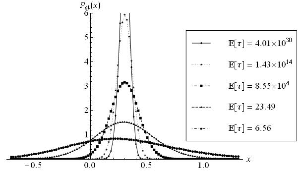
Many of the features of the first and second cases are repeated here, but with a longer tail of the distribution in the most diffuse case (from Eq.(34) the tail is seen to be power law suppressed).
3.3 Computing the MFPT
The MFPT, denoted by
is the expected value of the time taken for the process in Eq.(16) to hit a designated boundary ‘B’, with end points and , given that it begins inside the domain at initial time : . This is reminiscent of the considerations of [22] of on-off intermittency, the phenomenon of dynamical systems evolving in the vicinity of invariant manifolds and undergoing short bursts away from these manifolds.
The MFPT is calculated from the Andronov-Vitt-Pontryagin equation
| (36) |
where the initial position is varied keeping the position of the boundary fixed [11]. The boundary conditions encode that if the system starts on the boundary it takes zero time to cross it. The solution to Eq.(36) is elementary (see C for details),
| (37) |
In this paper, we pursue both numerical and, where possible, analytic computations of the MFPT given a solution to the Fokker-Planck equation. We use the latter to ensure understanding of the behaviour of the former. For numerical studies, -dependent choices of boundary values are straightforward. Similarly, we shall give formulae through the paper for general choices of , though we will concentrate on the minimal choice of for the most part. The legend in Fig.7 provides typical values of MFPT for Case III where this choice of . We observe that the curve with the highest MFPT () is, unsurprisingly, also the least diffuse: its variance is very narrow and the even tail is suppressed inside the region . The probability of the system being near or beyond the effective basin of attraction boundary is exponentially suppressed. Thus extremely long times must expire for the system to exit. The curve with is very similar. Nevertheless, even with small changes in the noise parameters the MFPT has decreased by 16 orders of magnitude. For the remaining plots we can see that the densities are becoming more diffuse and hence their MFPT values are quite small: large variances and long tails means that less time is needed for the system to leave the basin.
As a consequence of the strong peaks of distributions for low MFPT, we can further approximate the MFPT over times for which the decoupled system Eq.(15) is valid, before nonlinearities dominate the behaviour. This is achieved using the Laplace method, essentially saddle point integration of the integrals in Eq.(37). Recalling that we combined the key deterministic parameters in , it is similarly useful to combine stochastic parameters in
Setting and , we obtain the following approximation of the MFPT for the most general case (), for small values:
| (38) |
where,
and,
Details of the derivations of these expressions are given in C, where are kept general. This means that an -dependent choice may be implemented in analytical studies for specific graphs, as discussed earlier. The corresponding expression for is obtained by taking the limit. The expression for is then obtained by taking . In terms of and the corresponding limit is , such that .
4 MFPT and Stability: Analytical Results
We characterise our weaker notion of stochastic stability as
| (39) |
namely if the MFPT is greater than some externally selected threshold time, the system is deemed stable. We therefore restate our earlier question thus: if the system is deterministically stable, , what constraints must be imposed on the combinations of stochastic variables and so that the system also satisfies weak stochastic stability, Eq.(39)?
Since we are approximating at small MFPT, we can naturally find a condition for small . We simply apply Eq.(38) to Eq.(39) to obtain the inequality,
| (40) |
Eq.(40) constrains and such that, given and for deterministic stability and a choice for the period , the system satisfies weak stochastic stability. We shall illustrate more of its content below with the aid of numerical examples.
Insight into how to unpack Eq.(40) can be obtained by considering the Case I limit (, with ). For Eq.(40) we obtain a quadratic in given by:
| (41) |
In Eq.(41) we have discarded solutions which do not satisfy deterministic stability, Eq.(9). In Fig.8 we plot curves for different where Eq.(41) is an equality so that regions below/above a given curve represent weak stochastic stability/instability. The plots are readily understandable: larger values of mean a greater amount of time in which the noise can cause the system to drift out of the basin of attraction; thus lower noise levels, and a smaller area under the curve, are required to maintain stability. For a given value of , one can read thresholds in off curves such as Fig.8 such that stability is satisfied.
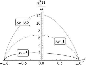
The approximate level curves in Fig.8 qualitatively emulate the corresponding exact equi-MFPT lines in Fig.9, including asymmetry. When considering Fig.9, for any given value of , given by the choice of , one considers a horizontal plane in the and axes. Any part of the horizontal plane which is inside its intersection with the surface is considered stable in the linear regime. Conversely, any part of the horizontal plane which is outside the intersection with the surface is considered unstable in the linear regime. The perimeter of the intersection of the surface and the horizontal plane gives the lines of equi-MFPT - these are approximately given in Fig.8 as parabola-like relationships between and .
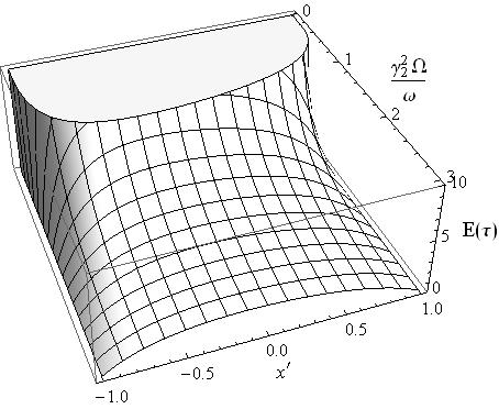
4.1 Case III MFPT
We examine the exact MFPT Eq.(37) for the noise of the general case III by plotting it against pairs of variables: MFPT against and , and MFPT against and . We focus on parameter ranges where the MFPT remains small. We consider three values of the correlation between zero and one.


As with Fig.8, when viewing Figs.10 and 11 for any given value of , one considers the corresponding linear plane with axes and in Fig.10 and axes and in Fig.11. Any part of the plane which is inside its intersection with the surface is considered stable in the linear regime. Conversely, any part of the plane which is outside its intersection with the surface is considered unstable in the linear regime. The perimeter of the intersection of the solid shape and the plane gives the lines of equi-MFPT. These are inverse-like relationships between and in Fig.10, and inverse-like relationships in and in Fig.11. The inverse-like relationship in both sets of graphs can be intuitively understood: as one of the stochastic parameters becomes large the other must be reduced to maintain stability.
With such plots one may now read off noise parameter thresholds such that weak stochastic stability is satisfied: choosing a threshold in MFPT (vertical axis), the area inside the curve represents stability and the area outside instability, so that noise parameter ranges can correspondingly be read off. For example, the ‘blob’ in the centre plots of Figs.10 and 11 indicates noise parameter values for which we earlier numerically solved the full Kuramoto model. We see from the plots that for any MFPT greater than one the parameter choice lies outside the region of stability. This is consistent with how quickly instabilities were typically generated for this noise choice, as seen, for example, in Figs.4.
4.2 Laplace approximation of Case III MFPT
To obtain an analytical bound for Eq.(40) we are required to make further approximations. It is straightforward to see (for example from expressions for the variance of the distributions) that small MFPT values are driven by small values of . Hence for we can apply to Eq.(40) the following simplification:
| (42) |
Inserting Eq.(42) into Eq.(40), we obtain the expression,
| (43) |
We notice that the LHS of Eq.(43) is quintic in and quartic in in contrast to the quadratic dependence on for case I.
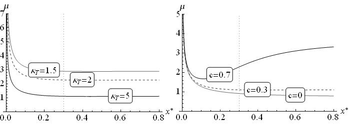
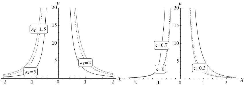
Obtaining regions of stability from Eq.(43) involves numerically solving for the roots of and . To compare against the plots in Figs.10 and 11 in the small MFPT regime we plot in Figs.12 and 13 the points where Eq.(43) becomes an equality against and , and against and . For the most part, the profiles based on the Laplace approximation for small MFPT qualitatively emulate those of the full MFPT computation in Fig.10. The exception is with the large result - right hand plot, Fig.12 - with a dip at low for which is not reproduced in the exact MFPT plot of Fig.10. This is readily understood as a region where the MFPT assumes intermediate values inconsistent with the approximations leading to Eq.(43). Similarly, the plots for small MFPT Fig.13 reproduce the shape of the equi-MFPT profiles of Fig.11 but finer details - the peak in Fig.13 is not as narrow as that in Fig.11 - are lost for intermediate MFPT values where the underlying approximations breakdown.
Generally then, there are interplays between and by which stochastic stability may be achieved for given and . But Eq.(43) provide now analytic expressions by which approximate thresholds may be determined, with finer calculation extracted from the full MFPT or refinements of these methods with higher order terms.
5 MFPT and Stability: Numerical
5.1 A conditional MFPT
In this section we study the behaviour of the stochastic Kuramoto model comparing switching off the noise based on our MFPT valid near-phase-synchronisation with switching off based on an MFPT for the full systeml Eq.(14). To determine an ‘exact’ MFPT we numerically solve Eq.(14), as discussed earlier, and collect the time for which each instance of first crosses the threshold . We then compute the mean over an ensemble of these values of time. The key issue is that, as said earlier, due to non-linear interactions switching on as the boundary of the basin of attraction is approached, many configurations in fact reach new stable positions inside the basin: the values are never reached. We must therefore collect a conditional sample: the time to reach the boundary for the set of configurations that do reach the boundary within the time for which we solve the system (we could also allow for extrapolations of trajectories beyond the maximum time for which we solve, which would give a yet longer MFPT). This is quite different from the MFPT we analytically compute, but gives us something with which to compare.
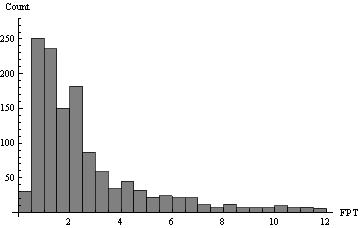
Fig.14 shows a histogram of this conditional sample. Denoting the expected value of the first passage time for over this conditioned sample , we obtain:
| (44) |
For the same values of noise parameters, the MFPT based on Eq.(37) (near phase-synchronisation, but no other approximations) gives:
| (45) |
The latter is less than the former, again, because non-linearities in the former lead to some trajectories never leaving the basin of attraction.
5.2 Switching off the noise
We now compare the impact of switching off the noise in time versus .

In Fig.15 we show the behaviour of the Kuramoto order parameter and the mode when noise is switched off at time , based on . In particular, we see the noise force the system out of the behaviour where the order parameter is close to one, and drop steadily (left hand plot). In most cases, the noise switches off before any chaotic dynamics emerge, and the deterministic synchronising dynamics resume, bringing the system back up to order parameter values of one, and modes back to the fixed point. However there is one instance where the destabilisation is sufficient that chaotic behaviour shows up in the order parameter (left hand plot, curve that drops lowest). Examining the mode in Fig.15 for this case (middle plot), we see that the mode reaches the edge of the basin - the outward trajectory is very clear - before the noise cuts out and most of the instances return to the original fixed point. Indeed, the instance for which the order parameter has shown an initial signal of chaos in the order parameter (left hand plot) corresponds to where attains a value very much larger than one (middle plot, highest curve), before reducing on cessation of the noise; in fact this instance returns to a copy of the original fixed point. Switching off the noise based on does not ‘save’ the system from some form of instability: individual modes are deflected sufficiently from the fixed point basin that they recouple and phase synchronisation is lost. However, the system always recovers upon cessation of the noise, as seen across a large number of instances in the right hand plot of Fig.15.

In contrast, switching off the noise at time , based on the MFPT from the near-phase-synchronised approximation shows no examples of instability. The impact of the noise is so slight that for the order parameter in Fig.16 (left hand plot) we must zoom into the behaviour near the value one to detect a deviation from full synchrony. Here, the time over which noise is applied is insufficient for interactions to switch back on, seen in the modes only slightly deflecting from steady-state values with none reaching values . Alternately, over the period for which noise is applied up to a time based on the MFPT, the approximation near phase synchrony is valid.
6 Summary and Discussion
We have shown that a threshold time for stability of phase synchronisation in the general network Kuramoto model subject to noise can be analytically computed using the Fokker-Planck formalism, leading to the Mean First Passage Time (MFPT). We have exploited a decomposition in graph Laplacian modes and a heuristic choice of boundary values of order one for the basin of attraction in these modes. The noise is applied additively and multiplicatively, with varying degrees of correlation. An approximation close to the phase synchronised fixed point has been critical to this. Because non-linear effects, outside our approximation, lead to unusual stabilisation effects, the MFPT is consistently an under-estimate (compared to, say, a conditional MFPT based on an ensemble of numerical solutions to the exact system that do leave the basin of attraction) of how long the noise can be sustained before instability is achieved. We gave arguments why for some large networks the boundary of the basin may be taken to scale with , and thus there is scope for allowing larger values of MFPT, but the choice of boundary of order one is sufficient to give a lower bound. The MFPT in the linearised system can therefore be used as a threshold for stability, allowing for analytic study of any undirected graph and frequency distribution. With these results one may determine conservative conditions on noise for stability for a given network and frequency distribution. Conversely one may use these results to test the robustness of a variety of networks for given values of noise.
On the basis of our results we can draw some broad implications for the behaviour of a variety known complex networks. For deterministic systems on easily disconnected graphs larger coupling is needed to stabilise phase synchronisation due to the ratio . With noise we have found that this ratio of deterministic parameters plays off against the combinations of stochastic parameters and . Our basic result is that level curves in MFPT show an inverse proportionality between these deterministic and stochastic parameters. This means that the same structural properties that make the system deterministically stable (lower ) also favour stochastic stability, thus allowing greater range of and . Specifically, for fixed coupling and frequencies, complex networks with a bulk of eigenvalues are both deterministically stable and robust against such a diversity of forms of noise. Dense Erdös-Rényi (if generated with high rewiring probability from a regular graph) and Small World graphs, have precisely such spectral properties [23]. Contrastingly, sparse Erdös-Rényi and Scale-Free graphs have Laplacian spectra with a ‘bulk’ in the region due to a large number of subgraphs disconnectable by a few link removals. Such graphs are, thus, more susceptible to stochastic instability.
This same mechanism may also explain for the deterministic Kuramoto model the synchronisability of particular graphs (how fast the graph reaches synchronisation rather than its stability once it gets there); for example, the Small-World graph is known to be more synchronisable [24]. Close to synchronisation but before onset of the linear regime, most of the low-lying Laplacian modes may be understood to be nearly quiescent generating a bath of noise on the remaining dynamical Laplacian modes. The synchronisability problem for the deterministic system may be recast as one of the system near phase synchronisation subject to noise, analogous to how a stochastic Kuramoto system can be derived from the deterministically chaotic Rössler system [25]; as with the Rössler system, one must make some strong assumptions to identify the noise as Gaussian White Noise in this way. In this respect, given our result that Small World networks are more stochastically stable, we can then infer that they are more synchronisable - thus providing a mechanism for the result in [24]
Over and above understanding the impact of noise on well-known complex networks, for us the power of our analytic results (or even numerically computing the MFPT from the solution to the Andronov-Vitt-Pontryagin equation) is that one may design networks to be robust against noise of specific levels.
To say more about transitions from phase synchronicity to alternative fixed points or meta-stable states (such as seen by [7, 8]) requires stochastically probing beyond first order approximations. For example, in our earlier work [10] we saw that second order approximations led to the Lotka-Volterra, rather than logistic, equations. This may help in understanding the non-linear stability behaviours we saw in numerical solutions of the exact system. It also offers the tantalising possibility of exploiting work on the impact of noise on multi-species competition dynamics to make more precise conclusions about phase synchronisation.
Acknowledgements
We thank Murray Batchelor, Richard Taylor, Tony Dekker and Markus Brede for valuable discussions and comments. This work was partly supported through the Internship program of the Australian Mathematical Sciences Institute (AMSI) and the Brazilian research agency FAPESP.
Appendix A The incidence matrix and ranges of Laplacian eigenmodes
We can relate each phase difference to the weighted sum of the eigenmodes , using the construct of the oriented incidence matrix defined as follows. Assign an arbitrary direction to each link of the original unoriented graph . The matrix elements of the oriented incidence matrix are given by
The Laplacian is then constructed by the following sum over links,
The structure means that the orientation plays no further role in the Laplacian of the original unoriented graph or its spectrum. However, the incidence matrix may be used to transform between objects respectively in the node and link spaces, including the Laplacian eigenvectors:
| (47) |
One can also use the incidence matrix to form a convenient expression for the difference of the phases connected by link between nodes and ,
| (48) |
In the above expression we have used the convention that link is incoming to node and outgoing to node . Applying to both sides of Eq.(47) and summing over all we can solve for to obtain,
| (49) |
Hence, beginning with Eq.(3) and Eq.(48), we can express the eigenmodes in terms of the phase differences, and the phase differences in terms of the eigenmodes respectively,
| (50) |
We see that Eq.(50) relates the difference of and with the sum of the difference of the eigenvectors, multiplied by the corresponding eigenmodes.
As stated earlier, the linear approximation to the sine interaction in the Kuramoto equation only holds when . To give some solid (albeit simplified) bounds, we consider a graph of nodes consisting of two equally sized complete graphs of order connected by a few bridging links around nodes . The Laplacian eigenvalues of this type of graph show marked differences with , and . The corresponding eigenvectors can then be characterised as follows:
We now consider the dynamical situation where the Kuramoto system is close to phase locked synchrony with all but one of the at steady-state values, , and seek the values of if the one dynamic approaches the value one. Taking as the dynamic mode, we obtain
| (53) |
The structure of the incidence matrix and eigenvectors leads to
where . Hence
in Eq.(53) since . We thus obtain
| (58) |
We see that is consistent with for all links, or a boundary in phase differences implies a boundary in of .
Contrastingly, if we consider the situation with one of , being dynamic but at steady state, we obtain
Labeling , we have,
| (62) |
We see now that can take values larger than one if . However, because are the corresponding Lyapunov exponents for these modes they are exponentially suppressed and will not lead to deviation from phase locked synchrony.
To illustrate these results we compare for the 27 node RB graph, a graph of 100 nodes form by joining two 50 node complete graphs, and one of 200 nodes formed by joining two 100 node complete graphs.

First we show how the values of vary if one of the all others taken at steady state values . In Fig.17 we show the scatter in across all links for a given value of for which . Note that, rather than generating new frequency spectra for each case here, we simply generate a random sample of values but bounded by . We see that in the RB graph (left panel) the modes have values suppressed, while for larger fluctuations phase differences can occur. However these are precisely the modes for which and therefore have fluctuations exponentially suppressed under Lyapunov stability. Contrastingly, for these larger fluctuations already occur at ; only for these graphs. We also see the periodicity of these larger fluctuations in units of , consistent with Eq.(62). Also in this plot, we see an -dependent suppression of when the mode reaching value one is .
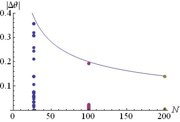
In Fig.18 we examine this lowest lying mode case, plotting against for all links . The suppression of by is evident.
Finally, at the other extreme, consider a complete graph. This has a completely spectrum of eigenvalues and all eigenvectors take the form of Eq.(A) and the boundary will scale with .
Appendix B Classical stochastic stability analysis of linear stochastic systems
Consider the general linear stochastic system,
| (63) |
Following Chapter 11 of [11], the classical concept of stability for a stochastic system is meaningful only when the fixed point, , is shared amongst and , i.e. . Due to linearity can be scaled to and we rewrite Eq.(63) as,
| (64) |
A system is classically stochastically stable if, given the matrices and , there exist symmetric positive-definite matrices and satisfying,
| (65) |
Focusing on the system given by Eq.(21) we see that,
and hence Eq.(65) becomes,
where we have mapped to for obvious convenience.
Because both and are diagonal we may take as the identity matrix. Thus, in order for to be a symmetric positive-definite, and thus for stochastic stability, we require
Appendix C Approximating the MFPT
C.1 Solving the Andronov-Vitt-Pontryagin equation)
C.2 Deriving approximate expressions
We now show how to obtain the approximation for given by Eq.(38). For this we use the Laplace Method, expected to work well when the arguments of the exponentials of the stationary densities have sharp turning points at the modes of the distributions. We begin at Eq.(66) and relabel,
| (67) |
We then Taylor expand and to second order around and - the points where . Hence,
where it is important to note that we assume that . Given the above approximations Eq.(66) becomes,
| (68) | |||||
where is an integration constant and erf is the error function.
We now concentrate on the quadratic exponontial term (expanded around ) multiplied by the error function (expanded around ) in Eq.(68). Eq.(67) assures us that for small , , and hence for the aforementioned exponential term we make the following further approximation,
This allows us to take advantage of the integral,
Thus Eq.(68) becomes,
| (71) | |||
| (74) | |||
| (75) |
where erfi is the complex error function. From , we obtain and,
In Eq.(75) we apply the asymptotic expansions for the complex error function and the hypergeometric function [27],
where . Hence Eq.(75) for small and becomes,
| (79) |
Eq.(79) is the expression used to generate the explicit form of the MFPT in the small valued regime, Eq.(38). Finally, using , and to stand for the respective cases (see Section 3.2), we have explicitly,
and,
References
- [1] Y Kuramoto, Chemical Oscillations, Waves and Turbulence, Springer, Berlin, (1984)
- [2] S H Strogatz, Physica D 143, (2000), 1
- [3] H Sakaguchi, Progr.Theor.Phys. 79, (1988), 39
- [4] S H Strogatz, R E Mirollo, J.Statist.Phys. 60, (1991), 613
- [5] J Gomez-Gardenes, Y Moreno, A Arenas, Phys.Rev.E 75, 066106 (2007); Phys.Rev.Lett. 98, 034101 (2007)
- [6] H Sakaguchi, Progr.Theoret.Phys. 79, (1988), 39
- [7] S H Park, S Kim, Phys.Rev.E 53, (1996), 3425
- [8] S Kim, S H Park, C S Ryu, Phys.Rev.Lett. 78, (1997), 1616
- [9] L M Pecora, T L Carroll, Phys.Rev.Lett. 80, (1998), 2109
- [10] A C Kalloniatis, Phys. Rev. E 82, 066202 (2010)
- [11] Z Schuss, Theory and applications of stochastic processes, Series in Applied Mathematical Sciences 170, Springer, New York, (2010)
- [12] P N McGraw, M Menzinger, Phys.Rev.E 77, 031102 (2008)
- [13] B Bollobás, Modern Graph Theory Springer, New York (1998)
- [14] M Fiedler, Czech. Math. J., 23, (1973), 298
- [15] E Ravasz, A L Barabási, Phys. Rev. E 67, 026112 (2003)
- [16] A Jadbabaie, N Motee, M Barahona, Proceedings of the American Control Conference, Vol. 5., (2004), 4296
- [17] F. Dörfler, F. Bullo, SIAM J. Applied Dynamical Systems, 10, (2011), 1070
- [18] P F Goŕa, Acta Physica Polonica B 36, No. 6, (2005), 1981
- [19] H Risken, The Fokker-Planck Equation, Springer-Verlag, Berlin (1984)
- [20] P.E. Kloeden, E. Platen, Numerical solution of stochastic differential equations, Springer, Berlin, Heidelberg, New York, 1999
- [21] V Linetsky, International Journal of Theoretical and Applied Finance, 7, No. 3, (2004), 337
- [22] S C Venkataramani, T M Antonsen Jr., E Ott, J C Sommerer, Physica D, 96, (1996), 66
- [23] A Jamakovic, P van Mieghem, European Conference on Complex Systems, 2006
- [24] H Hong, M Y Choi, B M Kim, Phys. Rev. E, 65, 026139 (2002)
- [25] A.S. Pikovsky, M.G. Rosenblum, G.V. Osipov, J. Kurths, Physica D 104 (1997), 219-238
- [26] B. Mohar, ”Some Applications of Laplace Eigenvalues in Graphs”, in Graph Symmetry: Algebraic Methods and Applications, Eds. G. Hahn, G. Sabidussi, NATO ASI Ser. C 497, Kluwer, 1997, pp. 225-275.
- [27] S K Kim, Mathematics of Computation, Volume 26, Number 120, (1972), 963