Numerical solutions of the coupled nonlinear Klein–Gordon equations by trigonometric integrator pseudospectral discretization

Abstract.

A scheme stemming from the use of pseudospectral approximations to spatial derivatives followed by a time integrator based on trigonometric polynomials is proposed for the numerical solutions of the coupled nonlinear Klein–Gordon equations. Numerical tests on one- and three-coupled Klein–Gordon equations are presented, which are geared towards understanding the accuracy and stability, and demonstrating the efficiency and high resolution capacity in application.

1. Introduction

The characteristics of nonlinear phenomena in various physics fields as, e.g., fluid dynamics, laser and fiber optics, solid state physics, plasma physics, chemical physics, reaction kinematics and etc., can be mathematically described by nonlinear evolution equations [1]. Among them of great physical significance are the equations that possess soliton solutions. In recent decades a variety of methods, such as the inverse scattering method [1, 2], bilinear transformation [12] and etc., have been developed for obtaining the exact solutions of soliton type equations. In parallel with the analytical treatment a surge of studies have been devoted to the numerics of these equations, which is a topic of great importance in applied science. In the present work the numerics of coupled nonlinear Klein–Gordon equations governing waves in a dispersive media is going to be examined.

$N$-coupled nonlinear Klein–Gordon equations under consider take the general form [3, 11]:

(1.1) $$\left(\frac{\partial^{2}}{\partial t^{2}}-\frac{\partial^{2}}{\partial x^{2}}\right)\psi_{k}+\psi_{k}-2\left(\sum_{p=1}^{N}\psi_{p}^{2}+Q\right)\psi_{k}=0,$$

(1.2) $$\left(\frac{\partial}{\partial t}-\frac{\partial}{\partial x}\right)Q+2\frac{\partial}{\partial t}\sum_{p=1}^{N}\psi_{p}^{2}=0,\quad x\in\mathbb{R},\quad t>0,$$

with $k=1,2,\ldots,N$, for $\psi_{k}(x,t)$ and $Q(x,t)$ sufficiently differentiable functions. Note that there exists an invariant of (1.1)-(1.2):

(1.3) $$E(t)=\int_{\mathbb{R}}\bigg{\{}\sum_{k=1}^{N}\left[\left(\partial_{t}\psi_{k}\right)^{2}+\left(\partial_{x}\psi_{k}\right)^{2}+\psi_{k}^{2}\right]-\bigg{(}\sum_{k=1}^{N}\psi_{k}^{2}\bigg{)}^{2}+\frac{1}{2}Q^{2}\bigg{\}}\mathrm{d}x,\quad t\geq 0,$$

and it suffices to refer the above conserved quantity as energy. Such conservation law can be justified from multiplying both sides of (1.1) by $2\partial_{t}\psi_{k}$ and, respectively, both sides of (1.2) by $Q$, integrating over $\mathbb{R}$ and then summing up for $k=1,2,\ldots,N$. Bilinear form and one-soliton solutions of (1.1)-(1.2) were investigated in [3, 11], and the complete integrability was also constructed from P-analysis [4, 15]. Along the numerical aspects of (1.1)-(1.2), to our best knowledge there are few results derived in literature.

The goal of this paper is to propose an efficient and accurate numerical scheme for solving (1.1)-(1.2). The key point in designing the scheme is based on applying Fourier pseudospectral approximations to the spatial derivatives, followed by applying a time integrator based on trigonometric polynomials, i.e., the so-called Gautschi-type or Deuflhard-type integrator (see e.g. [8, 10]) in phase space to the temporal discretization. The resulting scheme is fully explicit, symmetric in time, spectral-order of accuracy in space and second-order of accuracy in time, easy to implement and with less memory demand. Moreover, numerical tests demonstrate that the scheme is stable and conserves the energy defined by (1.3) very well, which are two favorable properties desired for a scheme in long-time simulation application. Note that the similar technique has been used for standard non-coupled Klein–Gordon equations [5], and for other classes of schemes, as for instance the finite-difference, decomposition and etc., for non-coupled Klein–Gordon equations we refer the readers to [6, 7, 9, 13, 14] and references given therein.

The rest is as follows. In Section 2 efficient numerical scheme is proposed. In Section 3 numerical results are reported for accuracy and stability tests of the scheme, and its application in numerically studying the dynamics of soliton-soliton collisions in one- and three-coupled Klein–Gordon equations. Finally some conclusions are drawn in Section 4.

2. Numerical scheme

In this section we shall propose the efficient numerical discretization. The initial conditions are assumed to be of the form:

(2.1) $$\psi_{k}(x,t=0)=\psi_{k}^{(0)}(x),\quad\partial_{t}\psi_{k}(k,t=0)=\psi_{k}^{(1)}(x),\quad Q(x,t=0)=Q^{(0)}(x),\quad x\in\mathbb{R}.$$

In practice we truncate the whole space problem into an interval $[a,b]$ with periodic boundary conditions

$$\psi_{k}(a,t)=\psi_{k}(b,t),\quad\partial_{x}\psi_{k}(a,t)=\partial_{x}\psi_{k}(b,t),\quad Q(a,t)=Q(b,t),\qquad t\geq 0.$$

Choose mesh size $h:=(b-a)/M$ with $M$ an even positive integer, time step $\tau>0$, and denote the grid points with coordinates $(x_{j},t_{n})=(a+jh,n\tau)$ for $j=0,1,\ldots,M$ and $n=0,1,\ldots$. Let $(\psi_{k})_{j}^{n}$ and $Q_{j}^{n}$ be the approximations of $\psi_{k}(x_{j},t_{n})$ and $Q(x_{j},t_{n})$, and denote by $\psi_{k}^{n}$ and $Q^{n}$ the solution vectors with components$(\psi_{k})_{j}^{n}$ and $Q_{j}^{n}$ respectively.

2.1. Discretization for (1.1)

Assume

(2.2) $$\psi_{k}(x,t)\approx\sum_{l=-M/2}^{M/2-1}\widetilde{(\psi_{k})}_{l}(t)\;~{}\mathrm{exp}\left(i\mu_{l}(x-a)\right),$$

for $a\leq x\leq b$ and $t\geq 0$, with $\mu_{l}=2\pi l/(b-a)$ ($l=-M/2,\ldots,M/2-1$) and $\widetilde{(\psi_{k})}_{l}(t)$ the discrete Fourier transformation coefficient of the $l$th mode,

(2.3) $$\widetilde{(\psi_{k})}_{l}(t)=\frac{1}{M}\sum_{j=0}^{M-1}\psi_{k}(x_{j},t)~{}\mathrm{exp}\left(-i\mu_{l}(x_{j}-a)\right),\quad l=-M/2,\ldots,M/2-1.$$

Approximating the spatial derivatives in (1.1) by Fourier pseudospectral discretization [16], i.e.,

$$-\partial_{xx}\psi_{k}(x,t)\approx\sum_{l=-M/2}^{M/2-1}\mu_{l}^{2}\widetilde{(\psi_{k})}_{l}(t)\;~{}\mathrm{exp}\left(i\mu_{l}(x-a)\right),$$

and noting orthogonality of the Fourier functions, we obtain the following second-order ODEs in phase space, for $l=-M/2,\ldots,M/2-1$,

(2.4) $$\frac{\mathrm{d}^{2}}{\mathrm{d}t^{2}}\widetilde{(\psi_{k})}_{l}(t)+\left(\mu_{l}^{2}+1\right)\widetilde{(\psi_{k})}_{l}(t)-\widetilde{\left(f_{k}\right)}_{l}(t)=0,$$

with $f_{k}(x,t)=2\left(\sum_{p=1}^{N}\psi_{p}^{2}(x,t)+Q(x,t)\right)\psi_{k}(x,t)$ and $\widetilde{\left(f_{k}\right)}_{l}(t)$ defined in an analogous way as (2.2). The analytical solutions of the above second-order ODEs can be written explicitly thanks to variation-of-constants formula. For $t_{n}$ (n=0,1,…) a given time,

$$\widetilde{(\psi_{k})}_{l}(t)= ~{}\widetilde{(\psi_{k})}_{l}(t_{n})\cos\left(\lambda_{l}(t-t_{n})\right)+\lambda_{l}^{-1}\frac{\mathrm{d}}{\mathrm{d}t}\widetilde{(\psi_{k})}_{l}(t_{n})\sin\left(\lambda_{l}(t-t_{n})\right)$$

(2.5) $$+\lambda_{l}^{-1}\int_{t_{n}}^{t}\widetilde{\left(f_{k}\right)}_{l}(s)\sin\left(\lambda_{l}(t-s)\right)\mathrm{d}s,$$

with $\lambda_{l}=\sqrt{\mu_{l}^{2}+1}$.

The approximations of $\psi_{k}(x,t_{1})$ are achieved from (2.5) with $n=0$ and $t=t_{1}=\tau$ together with the initial conditions (2.1) and approximating the integrals by standard trapezoidal rule. For $n=1,2,\ldots$, adding (2.5) with $t=t_{n+1}=t_{n}+\tau$ to its evaluation at $t=t_{n-1}=t_{n}-\tau$, and then approximating the integrals via trapezoidal rule, we get the three-term recurrence:

$$\widetilde{(\psi_{k})}_{l}(t_{n+1})= -\widetilde{(\psi_{k})}_{l}(t_{n-1})+2\widetilde{(\psi_{k})}_{l}(t_{n})\cos\left(\lambda_{l}\tau\right)$$

$$+\lambda_{l}^{-1}\int_{0}^{\tau}\left[\widetilde{\left(f_{k}\right)}_{l}(t_{n}+s)+\widetilde{\left(f_{k}\right)}_{l}(t_{n}-s)\right]\sin\left(\lambda_{l}(\tau-s)\right)\mathrm{d}s$$

(2.6) $$\approx -\widetilde{(\psi_{k})}_{l}(t_{n-1})+2\widetilde{(\psi_{k})}_{l}(t_{n})\cos\left(\lambda_{l}\tau\right)+\tau\lambda_{l}^{-1}\widetilde{\left(f_{k}\right)}_{l}(t_{n})\sin(\lambda_{l}\tau).$$

2.2. Discretization for (1.2)

Again, assuming

$$Q(x,t)\approx\sum_{l=-M/2}^{M/2-1}\widetilde{Q}_{l}(t)~{}~{}\mathrm{exp}\left(i\mu_{l}(x-a)\right),$$

for $a\leq x\leq b,\;t\geq 0$, and approximating the spatial derivative in (1.2) by Fourier pseudospectral discretization [16],

(2.7) $$\partial_{x}Q(x,t)\approx\sum_{l=-M/2}^{M/2-1}i\mu_{l}\widetilde{Q}_{l}(t)~{}~{}\mathrm{exp}\left(i\mu_{l}(x-a)\right),$$

we have the following first-order ODEs in phase space, for $l=-M/2,\ldots,M/2-1$,

(2.8) $$\frac{\mathrm{d}}{\mathrm{d}t}\widetilde{Q}_{l}(t)-i\mu_{l}\widetilde{Q}_{l}(t)=\frac{\mathrm{d}}{\mathrm{d}t}\widetilde{g}_{l}(t),$$

with $g(x,t)=-2\sum_{p=1}^{N}\psi_{p}^{2}(x,t)$. For $t_{n}$ ($n=0,1,\ldots$) a given time, integrating (2.8) from $t=t_{n}$ to $t=t_{n+1}=t_{n}+\tau$ and approximating the integrals via trapezoidal rule, we get,

$$\widetilde{Q}_{l}(t_{n+1})= ~{}~{}\mathrm{exp}\left(i\mu_{l}\tau\right)\widetilde{Q}_{l}(t_{n})+\widetilde{g}_{l}(t_{n+1})-~{}\mathrm{exp}\left(i\mu_{l}\tau\right)\widetilde{g}_{l}(t_{n})$$

$$+i\mu_{l}\int_{t_{n}}^{t_{n+1}}~{}\mathrm{exp}\left(i\mu_{l}(t_{n+1}-t)\right)\widetilde{g}_{l}(t)\mathrm{d}t$$

(2.9) $$\approx ~{}~{}\mathrm{exp}\left(i\mu_{l}\tau\right)\widetilde{Q}_{l}(t_{n})+\left(\frac{i\mu_{l}\tau}{2}+1\right)\widetilde{g}_{l}(t_{n+1})+\left(\frac{i\mu_{l}\tau}{2}-1\right)~{}\mathrm{exp}\left(i\mu_{l}\tau\right)\widetilde{g}_{l}(t_{n}).$$

2.3. Detailed numerical scheme

Choosing $(\psi_{k})^{0}_{j}=\psi_{k}^{(0)}(x_{j})$ and $Q_{j}^{0}=Q^{(0)}(x_{j})$, the detailed numerical scheme is as follows: for $n=1,2,\ldots$ and $j=0,1,\ldots,M$

(2.10) $$(\psi_{k})_{j}^{n}=\sum_{l=-M/2}^{M/2-1}\widetilde{\left(\psi_{k}^{n}\right)}_{l}~{}~{}\mathrm{exp}\left(\frac{2ijl\pi}{M}\right),$$

(2.11) $$Q_{j}^{n}=\sum_{l=-M/2}^{M/2-1}\widetilde{\left(Q^{n}\right)}_{l}~{}~{}\mathrm{exp}\left(\frac{2ijl\pi}{M}\right),$$

where,

(2.12) $$\widetilde{\left(\psi_{k}^{1}\right)}_{l}=\widetilde{\left(\psi_{k}^{(0)}\right)}_{l}\cos\left(\lambda_{l}\tau\right)+\widetilde{\left(\psi_{k}^{(1)}\right)}_{l}\lambda_{l}^{-1}\sin\left(\lambda_{l}\tau\right)+\frac{\tau}{2}\lambda_{l}^{-1}\widetilde{\left(f^{0}_{k}\right)}_{l}\sin\left(\lambda_{l}\tau\right),$$

(2.13) $$\widetilde{\left(\psi_{k}^{n+1}\right)}_{l}=-\widetilde{(\psi_{k}^{n-1})}_{l}+2\widetilde{(\psi_{k}^{n})}_{l}\cos\left(\lambda_{l}\tau\right)+\tau\lambda_{l}^{-1}\widetilde{\left(f_{k}^{n}\right)}_{l}\sin(\lambda_{l}\tau),\quad n=1,2,\ldots,$$

$$\widetilde{\left(Q^{n+1}\right)}_{l}=~{}\mathrm{exp}\left(i\mu_{l}\tau\right)\widetilde{\left(Q^{n}\right)}_{l}+\left(\frac{i\mu_{l}\tau}{2}+1\right)\widetilde{\left(g^{n+1}\right)}_{l}$$

(2.14) $$\qquad\qquad+\left(\frac{i\mu_{l}\tau}{2}-1\right)~{}\mathrm{exp}\left(i\mu_{l}\tau\right)\widetilde{\left(g^{n}\right)}_{l},\quad n=0,1,\ldots.$$

Here, the vector $f_{k}^{n}=\left[\left(f_{k}\right)_{0}^{n},\left(f_{k}\right)_{1}^{n},\ldots,\left(f_{k}\right)_{M}^{n}\right]^{T}$ and $g^{n}=\left[g^{n}_{0},g^{n}_{1},\ldots,g^{n}_{M}\right]^{T}$ are defined by

$$\left(f_{k}\right)_{j}^{n}=2\left(\sum_{p=1}^{N}\left(\left(\psi_{p}\right)^{n}_{j}\right)^{2}+Q_{j}^{n}\right)\left(\psi_{k}\right)^{n}_{j},\qquad g^{n}_{j}=-2\sum_{p=1}^{N}\left(\left(\psi_{p}\right)^{n}_{j}\right)^{2}.$$

If the energy defined by (1.3) is of interests, then the approximation of $\partial_{t}\psi_{k}(x_{j},t_{n})$,

(2.15) $$(\phi_{k})_{j}^{n}=\sum_{l=-M/2}^{M/2-1}\widetilde{\left(\phi_{k}^{n}\right)}_{l}~{}~{}\mathrm{exp}\left(\frac{2ijl\pi}{M}\right),$$

for $j=0,1,\ldots,M$ and $n=1,2,\ldots$ can be obtained from

(2.16) $$\widetilde{\left(\psi_{k}^{n+1}\right)}_{l}-\widetilde{\left(\psi_{k}^{n-1}\right)}_{l}=2\lambda_{l}^{-1}\widetilde{\left(\phi_{k}^{n}\right)}_{l}\sin\left(\lambda_{l}\tau\right),$$

which is achieved by subtracting (2.5) with $t=t_{n+1}=t_{n}+\tau$ from its evaluation at $t=t_{n-1}=t_{n}-\tau$, and applying trapezoidal rule to the integrals.

The scheme (2.10)-(2.16) is fully explicit, symmetric in time by noting that it is unchanged if we interchange $\tau\leftrightarrow-\tau$ and $n\leftrightarrow n+1$, and quite efficient in implementation thanks to FFT. It is of spectral-order of accuracy in space, i.e., it converges exponentially fast as mesh size refined smaller, which is an expected property for the spectral-type discretization. Moreover, as shown by numerical experiments reported in the next section, the scheme is of second-order of accuracy in time, stable and conserves the energy defined by (1.3) very well.

3. Numerical results

Numerical examples are reported in this section towards understanding the accuracy and stability of the numerical scheme (2.10)-(2.16), and applying it to study soliton-soliton collisions in one- and three-coupled nonlinear Klein–Gordon equations.

Table 1. Accuracy tests results: (i) upper part for discretization error in space, under $\tau=0.0001$; (ii) middle part for discretization error in time, under $h=1/8$ and (iii) lower part for conserved quantity analysis, under $h=1/4$ and $\tau=0.02$.

	$h=1/2$	$h=1/4$	$h=1/8$	$h=1/16$
$e(60)$	1.1677E-1	2.8638E-6	1.7098E-6	1.0244E-8
	$\tau=0.04$	$\tau=0.02$	$\tau=0.01$	$\tau=0.005$
$e(60)$	1.1654E-1	2.9405E-2	7.3659E-3	1.8423E-3
$t$	$t=50$	$t=100$	$t=150$	$t=200$
$E(t)$	0.67890052	0.67890052	0.67890050	0.67890051

3.1. Accuracy tests and stability study

It is known that the $N$-coupled nonlinear Klein–Gordon equations admit the following analytical one-soliton solutions [3]:

(3.1) $$\psi_{(c,\;\alpha_{k})}(x,t)=\alpha_{k}\sqrt{\frac{1+c}{1-c}}~{}\mathrm{sech}\left(\frac{x-ct}{\sqrt{1-c^{2}}}\right),$$

(3.2) $$Q_{c}(x,t)=\frac{2c}{c-1}~{}\mathrm{sech}^{2}\left(\frac{x-ct}{\sqrt{1-c^{2}}}\right),$$

with $\left|c\right|<1$ an arbitrary constant, and coefficients $\alpha_{k}$ satisfying $\sum_{k=1}^{N}\alpha_{k}^{2}=1$. To test the accuracy, we solve the one-coupled nonlinear Klein–Gordon equations (i.e. $N=1$ in (1.1)-(1.2)) on $[-24,104]$ for $0\leq t\leq 200$, with initial data $\psi_{1}^{(0)}(x)=\psi_{(0.4,\;1)}(x,t=0)$, $\psi_{1}^{(1)}(x)=\partial_{t}\psi_{(0.4,\;1)}(x,t=0)$ and $Q^{(0)}(x)=Q_{0.4}(x,t=0)$. To quantify the numerical results, the error function $e(t)$ is defined as the maximum error, $e(t_{n}):=\max_{j}\left|(\psi_{1})^{n}_{j}-\psi_{1}(x_{j},t_{n})\right|+\max_{j}\left|Q^{n}_{j}-Q(x_{j},t_{n})\right|$.

 

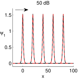
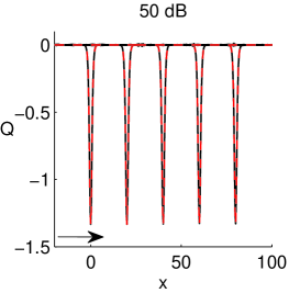
Figure 1. Comparisons between numerical one-soliton results (solid line) from initial data perturbed by adding white Gaussian noise with signal-to-noise ratio 50dB and results (dashed line and red colored online) from initial data without perturbation, under $h=1/4$ and $\tau=0.02$. Wave fronts depicted for $t=0,~{}50,~{}100,~{}150$ and $200$ (from left to right).

To test the discretization error in space, we choose a very fine time step $\tau=0.0001$ such that the error from time discretization is negligible compared to the spatial discretization error. Similarly, we choose a very fine mesh size $h=1/8$ to eliminate the spatial discretization error for testing the discretization error in time. Also, mesh size $h=1/4$ and time step $\tau=0.02$ are chosen to test the conservation of conserved quantity (1.3). The results are listed in Table 1. To study the stability of the scheme, the same initial conditions as chosen previously are used, to which we add white Gaussian noise with signal-to-noise ratio 50dB. The results are depicted in Figure 1.

Based on these results, the following are drawn:

1. The numerical scheme (2.10)-(2.16) is of spectral-order of accuracy in space, i.e., its convergence order in space is higher than any polynomial order, and of second-order of accuracy in time.

2. It conserves the invariant defined by (1.3) very well (up to seven significant digits in the reported example) over a long-time simulation.

3. It is numerically stable, by which we mean a minor perturbation in the initial data dose not bring in significant difference to the results over a long-time simulation and no numerical blow-up occurs.

3.2. Applications on soliton-soliton collisions

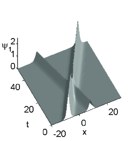
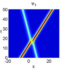
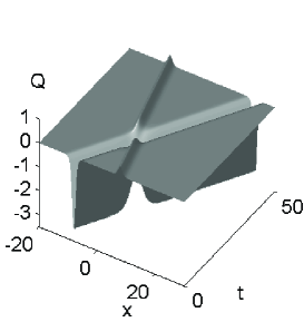
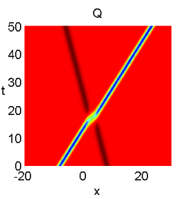
Figure 2. Numerical results for soliton-soliton collisions in one-coupled Klein–Gordon equations. Left column for solution evolution and right column for its contours (color online). Computations are carried out on $[-24,40]$ under $h=1/4$ and $\tau=0.02$. Initial conditions are chosen as (3.3)-(3.5) with $x_{0}=8$ such that initially two one-soliton waves are well separated.

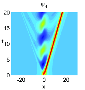
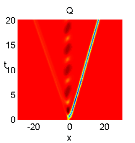
Figure 3. Contours (color online) of numerical results for soliton-soliton collisions in one-coupled Klein–Gordon equations. Computations are carried out on $[-32,32]$ under $h=1/4$ and $\tau=0.02$. Initial conditions are chosen as (3.3)-(3.5) with $x_{0}=1$ such that initially two one-soliton waves are almost at the same location.

First we apply the method to one-coupled nonlinear Klein–Gordon equations, i.e., $N=1$ in (1.1)-(1.2), with initial date:

(3.3) $$\psi_{1}^{(0)}(x)=\psi_{(0.6,\;1)}(x+x_{0},t=0)+\psi_{(-0.25,\;1)}(x-x_{0},t=0),$$

(3.4) $$\psi_{1}^{(1)}(x)=\partial_{t}\psi_{(0.6,\;1)}(x+x_{0},t=0)+\partial_{t}\psi_{(-0.25,\;1)}(x-x_{0},t=0),$$

(3.5) $$Q^{(0)}(x)=Q_{0.6}(x+x_{0},t=0)+Q_{-0.25}(x-x_{0},t=0),$$

with a dislocation parameter $x_{0}>0$ to measure the separation of two one-soliton waves at initial time level. Some results from numerical experiments are shown in Figure 2 and Figure 3. These results indicate that when two solitons are of nearly completed separation at initial time level, after the collision the solutions remain to propagate in soliton pattern as the time proceeds and there is no visible wave structure emitted. On the other hand, when two solitons are not quite separated at initial time level, after the collision the emission of new waves is conspicuous.

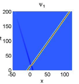
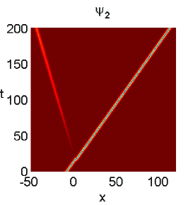
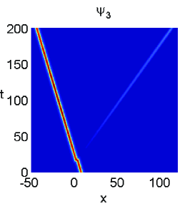
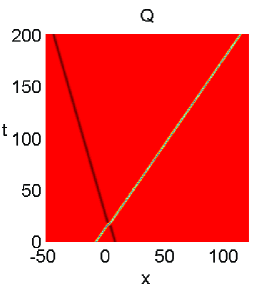
Figure 4. Contours (color online) of numerical results for soliton-soliton collisions in three-coupled Klein–Gordon equations. Computations are carried out on $[-96,160]$ under $h=1/4$ and $\tau=0.02$. Initial conditions are chosen as (3.6)-(3.12) with $x_{0}=8$ such that initially two one-soliton waves are well separated.

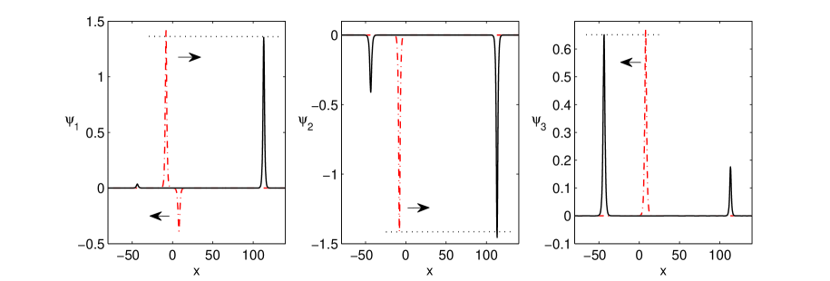
Figure 5. Numerical results of $\psi_{1}$, $\psi_{2}$ and $\psi_{3}$ for soliton-soliton collisions in three-coupled Klein–Gordon equations: solid line corresponds to time $t=200$ and dash-dot line (red colored online) corresponds to time $t=0$. Parameters are same as Figure 4.

Next we present an example of applying the method to three-coupled nonlinear Klein–Gordon equations, i.e., $N=3$ in (1.1)-(1.2), and the initial conditions are taken as

(3.6) $$\psi_{1}^{(0)}(x)=\psi_{(0.6,\;1/\sqrt{2})}(x+x_{0},t=0)+\psi_{(-0.25,\;-1/2)}(x-x_{0},t=0),$$

(3.7) $$\psi_{2}^{(0)}(x)=\psi_{(0.6,\;-1/\sqrt{2})}(x+x_{0},t=0),$$

(3.8) $$\psi_{3}^{(0)}(x)=\psi_{(-0.25,\;\sqrt{3}/2)}(x-x_{0},t=0),$$

(3.9) $$\psi_{1}^{(1)}(x)=\partial_{t}\psi_{(0.6,\;1/\sqrt{2})}(x+x_{0},t=0)+\partial_{t}\psi_{(-0.25,\;-1/2)}(x-x_{0},t=0),$$

(3.10) $$\psi_{2}^{(1)}(x)=\partial_{t}\psi_{(0.6,\;-1/\sqrt{2})}(x+x_{0},t=0),$$

(3.11) $$\psi_{3}^{(1)}(x)=\partial_{t}\psi_{(-0.25,\;\sqrt{3}/2)}(x-x_{0},t=0),$$

(3.12) $$Q^{(0)}(x)=Q_{0,6}(x+x_{0},t=0)+Q_{-0.25}(x-x_{0},t=0),$$

again with a dislocation parameter $x_{0}>0$ to measure the separation of two one-soliton waves at initial time level. Some results from numerical experiments are depicted in Figure 4 and Figure 5, in which initially two soliton waves are well separated and only a wave front moving towards the right $x$-axis exists in $\psi_{2}$ while only a wave front moving towards the left $x$-axis exists in $\psi_{3}$. It shows that after the collision a new wave front moving towards the left $x$-axis appears in $\psi_{2}$ and a new wave front moving towards the right $x$-axis appears in $\psi_{3}$. Also, a conspicuous change in the amplitude of waves is observed, see Figure 5. Results for two solitons not separated at initial time level are quite similar as in one-coupled Klein–Gordon equations.

The results presented in this section indicate that the dynamics of waves governed by coupled nonlinear Klein–Gordon equations is a rather complicated issue. The results also demonstrate the efficiency and high resolution of the proposed method for numerically studying the coupled nonlinear Klein–Gordon equations.

4. Conclusions

A numerical scheme, which is based on the application of pseudospectral approximations to spatial derivatives followed by a trigonometric integrator to temporal discretization in phase space, was proposed for solving coupled nonlinear Klein–Gordon equations. The soliton solutions arising from one-coupled Klein–Gordon equations were examined to test the accuracy and stability. Also, application results of studying soliton-soliton collisions in one- and three-coupled Klein–Gordon equations were reported as examples to demonstrate the efficiency and high resolution of the scheme.

References

- [1] M.J. Ablowitz and P.A. Clarkson, Solitons, nonlinear evolution equations and inverse scattering transform, Cambridge University Press, Cambridge, 1990.
- [2] M.J. Ablowitz and H. Segur, Solitons and inverse scattering transformation, SIAM, Philadelphia, 1981.
- [3] T. Alagesan, Y. Chung and K. Nakkeeran, Soliton solutions of coupled nonlinear Klein–Gordon equations, Chaos Solitions Fract. 21 (2004) 879–882.
- [4] T. Alagesan, Y. Chung and K. Nakkeeran, Painlevé analysis of -coupled nonlinear Klein–Gordon equations, J. Phys. Soc. Jpn. 72 (2003) 1818.
- [5] W. Bao and X. Dong, Analysis and comparison of numerical methods for Klein–Gordon equation in nonrelativistic limit regime, Numer. Math. (in press) DOI 10.1007/s00211-011-0411-2.
- [6] W. Cao and B. Guo, Fourier collocation method for solving nonlinear Klein–Gordon equation, J. Comput. Phys. 108 (1993) 296–305.
- [7] E.Y. Deeba and S.A. Khuri, A decomposition method for solving the nonlinear Klein–Gordon equation, J. Comput. Phys. 124 (1996) 442–448.
- [8] P. Deuflhard, A study of extrapolation methods based on multistep schemes without parasitic solutions, Z. Angew. Math. Phys. 30 (1979) 177–189.
- [9] D.B. Duncan, Symplectic finite difference approximations of the nonlinear Klein–Gordon equation, SIAM J. Numer. Anal. 34 (1997) 1742–1760.
- [10] W. Gautschi, Numerical integration of ordinary differential equations based on trigonometric polynomials, Numer. Math. 3 (1961) 381–397.
- [11] H. Hirota and Y. Ohta, Hierarchies of coupled soliton equations. I, J. Phys. Soc. Jpn. 60 (1991) 798–809.
- [12] R. Hirota, Direct method of finding exact solutions of nonlinear evolution equations, Lect. Notes Math., vol. 515, pp. 40–68, Springer, Berlin-Heidelberg-New York, 1976.
- [13] S. Li and L. Vu-Quoc, Finite difference calculus invariant structure of a class of algorithms for the nonlinear Klein–Gordon equation, SIAM J. Numer. Anal. 32 (1995) 1839–1875.
- [14] P.J. Pascual, S. Jiménez and L. Vázquez, Numerical simulations of a nonlinear Klein–Gordon model. Applications, Lect. Notes Phys., vol. 448, pp. 211–270, Springer, Berlin, 1995.
- [15] K. Porsezian and T. Alagesan, Painlevá analysis and complete integrability of coupled Klein–Gordon equations, Phys. Lett. A 198 (1995) 378–382.
- [16] J. Shen and T. Tang, Spectral and High-Order Methods with Applications, Science Press, Beijing, 2006.