Pricing Derivatives on Multiscale Diffusions: an Eigenfunction Expansion Approach

Abstract

Using tools from spectral analysis, singular and regular perturbation theory, we develop a systematic method for analytically computing the approximate price of a large class derivative-assets. The payoff of the derivative-assets may be path-dependent. Additionally, the process underlying the derivatives may exhibit killing (i.e., jump to default) as well as combined local/nonlocal stochastic volatility. The nonlocal component of volatility may be multiscale, in the sense that it may be driven by one fast-varying and one slow-varying factor. The flexibility of our modeling framework is contrasted by the simplicity of our method. We reduce the derivative pricing problem to that of solving a single eigenvalue equation. Once the eigenvalue equation is solved, the approximate price of a derivative can be calculated formulaically. To illustrate our method, we calculate the approximate price of three derivative-assets: a vanilla option on a defaultable stock, a path-dependent option on a non-defaultable stock, and a bond in a short-rate model.

Keywords: derivative pricing, stochastic volatility, local volatility, default, knock-out, barrier, spectral theory, eigenfunction, singular perturbation theory, regular perturbation theory.

1 Introduction

The spectral representation for the transition density of a general one-dimensional diffusion was obtained in a seminal paper by McKean (1956). Since that time, spectral theory – and more specifically, the study of eigenfunction expansions of linear operators – has become an essential tool for analysing diffusions. As a diffusion often serves as the underlying process on which financial models are built, it is not surprising that methods from spectral theory have made their way into mathematical finance as well.

In particular, many problems related to the pricing of derivative-assets have been solved analytically by using methods from spectral theory. An overview of the spectral method applied to derivative pricing is as follows. Using risk-neutral pricing, one expresses the value of a derivative-asset $u(t,x)$ as a risk-neutral expectation of some function of the future value of an underlying process $X$. Mathematically, this is expressed as

(1.1) $$u(t,x)=\widetilde{\mathbb{E}}_{x}[H(X_{t})]=\int H(y)\,p(t,x,y)\,dy.$$

Here, $p(t,x,y)$ is the transition density of the $X$ under $\widetilde{\mathbb{P}}$. If it turns out that the ininitesmal generator $\mathscr{L}$ of the underlying process is self-adjoint on a Hilbert space with weighting measure $m(x)dx$ and if the spectrum of $\mathscr{L}$ is purely discrete, then the transition density of $X$ has an eigenfunction expansion

(1.2) $$p(t,x,y)=m(y)\sum_{n}e^{-\lambda_{n}t}\psi_{n}(y)\psi_{n}(x),$$

where $\left\{\lambda_{n}\right\}$ are the eigenvalues of $(-\mathscr{L})$ and $\left\{\psi_{n}\right\}$ are the corresponding eigenfunctions

(1.3) $$-\mathscr{L}\,\psi_{n}=\lambda_{n}\,\psi_{n}.$$

The value of a derivative-asset can then be expressed analytically by inserting (1.2) into (1.1)

(1.4) $$u(t,x) =\sum c_{n}\,e^{-\lambda_{n}t}\,\psi_{n}(x), c_{n} =\left(\psi_{n},H\right):=\int H(y)\psi_{n}(y)m(y)dy.$$

Under some basic assumptions, the infinitesimal generator of a general one-dimensional diffusion

(1.5) $$\mathscr{L} =\frac{1}{2}a^{2}(x)\partial^{2}_{xx}+b(x)\partial_{x}-k(x), x \in(e_{1},e_{2}),$$

with domain $\text{dom}(\mathscr{L})$ (described in appendix A.2) is always self-adjoint on the Hilbert space $\mathscr{H}=L^{2}(I,\mathfrak{m})$, where $I\subset\mathbb{R}$ is an interval with endpoints $e_{1}$ and $e_{2}$ and $\mathfrak{m}$ is the speed density of the diffusion

(1.6) $$\mathfrak{m}(x) :=\frac{2}{a^{2}(x)}\exp\left(\int_{x_{0}}^{x}\frac{2\,b(y)}{a^{2}(y)}dy\right). (\text{speed density)}$$

The lower limit of integration $x_{0}\in I$ is arbitrary. Thus, when a one-dimensional diffusion is adequate for describing the dynamics of an underlying, the spectral method outlined above serves as a powerful tool for analytically pricing derivatives on that underlying. Among the topics that have been addressed by applying spectral methods to one-dimensional diffusions are option pricing (both vanilla and exotic), mortgages valuation, interest rate modeling, volatility modeling, and credit risk (see Davydov and Linetsky (2001); Linetsky (2002); Davydov and Linetsky (2003); Linetsky (2004b); Albanese and Lawi (2005); Albanese and Kuznetsov (2004); Albanese, Campolieti, Carr, and Lipton (2001); Lewis (1998); Lipton and McGhee (2002); Goldstein and Keirstead (1997); Gorovoi and Linetsky (2004); Gorovoy and Linetsky (2007); Carr and Linetsky (2006); Linetsky (2004a, c, 2006)). A useful reference on the topic of spectral methods for one-dimensional diffusions in finance is Linetsky (2007).

As widely applicable as one-dimensional diffusions are in finance, there are applications in which one-dimensional diffusions are not adequate for describing the dynamics of an underlying. This is the case, for example, in a stochastic volatility setting, where the volatility of the asset that underlies a derivative is controlled by (possibly multiple) nonlocal diffusions. Ideally, one would like to employ techniques from spectral theory to solve problems that relate to multidimensional diffusions. Unfortunately, whereas the infinitesimal generator of a one-dimensional diffusion is practically guaranteed to be self-adjoint, the infinitesimal generator of a multidimensional diffusion is only self-adjoint when the drift vector satisfies certain constraints imposed by the volatility matrix. The drift constraint is not satisfied by any of the most prominent stochastic volatility models – Heston (1993), Hull and White (1987), Stein and Stein (1991) and the SABR model by Hagan, Kumar, Lesniewski, and Woodward (2002) – which complicates the use of spectral methods.

Recently, Fouque, Jaimungal, and Lorig (2011), show one way to deal with this issue. By combining techniques from singular perturbation theory and spectral theory, the authors are able to express the approximate price of a (possibly path-dependent) option as an eigenfunction expansion, even though the infinitesimal generator of the two-dimensional diffusion they work with is not self-adjoint. As notable as their work is, the results of Fouque, Jaimungal, and Lorig (2011) are valid only when the asset underlying the option is a Black-Scholes-like geometric Brownian motion (GBM) with fast mean-reverting stochastic volatility.

In this paper, we extend the work of Fouque, Jaimungal, and Lorig (2011) in four important ways.

1. As a “base” model, we work with a general one-dimensional diffusion $dX_{t}=\nu(X_{t})dt+a(X_{t})dW_{t}$. This is in contrast to Fouque, Jaimungal, and Lorig (2011), where the only base model considered is a GBM: $dX_{t}=\mu X_{t}dt+\sigma X_{t}dW_{t}$.

2. The general diffusion we work with may exhibit killing (jump to default) at a rate $h(X_{t})\geq 0$. In the GBM case considered in Fouque, Jaimungal, and Lorig (2011), $X$ is always strictly positive.

3. To our general diffusion we add two factors of nonlocal volatility: $a(X_{t})\rightarrow a(X_{t})f(Y_{t},Z_{t})$. The first factor $Y$ is a fast-varying factor. The second factor $Z$ is slow-varying. Thus, our model is a multiscale stochastic volatility model. Again, this is in contrast to Fouque, Jaimungal, and Lorig (2011), where the analysis is limited to a single fast mean-reverting factor of volatility $\sigma X_{t}\rightarrow f(Y_{t})X_{t}$.

4. In changing from the physical probability measure to the risk-neutral pricing measure, we consider a class of market prices of risk that is general enough to treat credit, equity, and interest rate derivatives in a single framework. In Fouque, Jaimungal, and Lorig (2011) the form chosen for the market price of risk restricts the authors to equity derivatives only.

As in Fouque, Jaimungal, and Lorig (2011), we will derive an eigenfunction expansion for the approximate price of a derivative-asset despite the fact that the infinitesimal generator we consider is not (in general) self-adjoint. Unlike Fouque, Jaimungal, and Lorig (2011), because our multidimensional diffusion contains both a fast-varying and a slow-varying factor of volatility, we must combine techniques from both singular and regular perturbation theory to achieve our result. In Fouque, Jaimungal, and Lorig (2011), only singular perturbation techniques are required, due to the presence of a single fast mean-reverting factor of volatility.

Of course, the idea of combining singular and regular perturbation techniques in a multiscale stochastic volatility setting is not particularly new or unique. The seminal paper on the subject, applied in a Black-Scholes-like GBM setting, is due to Fouque, Papanicolaou, Sircar, and Sølna (2004). Further application of the singular and regular perturbation methods developed in Fouque, Papanicolaou, Sircar, and Sølna (2004) led to papers concerning bond-pricing, interest rate derivatives, credit derivatives, and option pricing in a CEV-like setting (see DeSantiago, Fouque, and Sølna (2008); Cotton, Fouque, Papanicolaou, and Sircar (2004); Fouque, Sircar, and Sølna (2006, 2008); Choi, Fouque, and Kim (2010)). There is also a book by Fouque, Papanicolaou, Sircar, and Solna (2011), which contains the many of the key results from the above mentioned publications. What this paper contributes to the existing literature on multiscale diffusions is flexibility and simplicity. From a flexibility standpoint, the methods developed in this paper are able to encapsulate, in a unified framework, many of the results contained in Choi, Fouque, and Kim (2010); Cotton, Fouque, Papanicolaou, and Sircar (2004); DeSantiago, Fouque, and Sølna (2008); Fouque, Sircar, and Sølna (2006); Fouque, Papanicolaou, Sircar, and Sølna (2004, 2011); Fouque, Wignall, and Zhou (2008), as well as further results, which are not contained in these works (e.g., jump to default CEV with multiscale stochastic volatility, see section 4.3). With regards to simplicity, the spectral method we develop reduces the derivative pricing problem to that of solving a single, one-dimensional eigenvalue equation. Once this equation is solved, the approximate price of a derivative-asset can be calculated formulaically by computing a few simple inner products. This is in contrast to the methods developed in Choi, Fouque, and Kim (2010); Cotton, Fouque, Papanicolaou, and Sircar (2004); DeSantiago, Fouque, and Sølna (2008); Fouque, Sircar, and Sølna (2006); Fouque, Papanicolaou, Sircar, and Sølna (2004, 2011); Fouque, Wignall, and Zhou (2008), where, in order to express the approximate price of a derivative-asset, an inhomogeneous partial differential equation (PDE) must be solved.

The rest of this paper proceeds as follows. In section 2 we introduce a class of models described by multiscale diffusions. We also explain the kind of derivative-asset we wish to consider. In section 3 we solve (approximately), the problem of pricing a derivative-asset. This is done in several steps. First, using risk-neutral pricing, we derive a Cauchy problem which, if solved, would yield the exact value of a derivative-asset. Next, we use techniques from singular and regular perturbation theory to formally derive three simpler Cauchy problems, which, if solved, would yield the approximate value of a derivative-asset. Finally, using eigenfunction expansion techniques, we solve these Cauchy problems explicitly. The solutions are given in Theorems 3.1, 3.2 and 3.3. In section 4, we illustrate our method of pricing derivative-assets with three examples. We also provide an appendix, which contains some mathematical results that we use throughout this paper.

2 A Class of Multiscale Models

Let $(\Omega,\mathscr{F},\mathbb{P})$ be a probability space supporting correlated Brownian motions $(W^{x},W^{y},W^{z})$ and an exponential random variable $\mathscr{E}\sim\text{Exp}(1)$, which is independent of $(W^{x},W^{y},W^{z})$. We shall consider a three-factor economy described by a time-homogenous, continuous-time Markov process $\mathscr{X}=(X,Y,Z)$, which takes values in some state space $E=I\times\mathbb{R}\times\mathbb{R}$. Here, $I$ is an interval in $\mathbb{R}$ with endpoints $e_{1}$ and $e_{2}$ such that $-\infty\leq e_{1}<e_{2}\leq\infty$. We assume that $\mathscr{X}$ starts in $E$ and is instantaneously killed (sent to an isolated cemetery state $\Delta$) as soon as $X$ leaves $I$. Specifically, the dynamics of $\mathscr{X}$ under the physical measure $\mathbb{P}$ are as follows:

(2.1) $$\mathscr{X}_{t} =\begin{cases}\left(X_{t},Y_{t},Z_{t}\right)&\tau_{I}>t\\ \Delta&\tau_{I}\leq t\end{cases}, \tau_{I} =\inf\left\{t>0:X_{t}\notin I\right\},$$

where $\left(X,Y,Z\right)$ are given by

(2.2) $$\left\{\begin{aligned} dX_{t}&=\nu(X_{t})\,dt+a(X_{t})f(Y_{t},Z_{t})\,dW^{x}_{t},\\ dY_{t}&=\frac{1}{\epsilon}\alpha(Y_{t})dt+\frac{1}{\sqrt{\epsilon}}\beta(Y_{t})\,dW^{y}_{t},\\ dZ_{t}&=\delta c(Z_{t})dt+\sqrt{\delta}g(Z_{t})\,dW^{z}_{t},\\ d\left\langle W^{x},W^{y}\right\rangle_{t}&=\rho_{xy}\,dt,\\ d\left\langle W^{x},W^{z}\right\rangle_{t}&=\rho_{xz}\,dt,\\ d\left\langle W^{y},W^{z}\right\rangle_{t}&=\rho_{yz}\,dt,\\ (X_{0},Y_{0},Z_{0})&=(x,y,z)\in E.\end{aligned}\right.$$

Here, $(\rho_{xy},\rho_{xz},\rho_{yz})$ satisfy $|\rho_{xy}|,|\rho_{xz}|,|\rho_{yz}|\leq 1$ and $1+2\rho_{xy}\rho_{xz}\rho_{yz}-\rho_{xy}^{2}-\rho_{xz}^{2}-\rho_{yz}^{2}\geq 0$ so that the correlation matrix of the Brownian motions is positive-semidefinite.

The process $X$ could represent a variety of things. For example, it could represent the price of a stock, the value of an index, the risk-free short-rate of interest, etc. More generally, $X$ could represent an exogenous factor that controls the value of any or all of the items mentioned above. Under the physical measure $\mathbb{P}$, the process $X$ has instantaneous drift $\nu(X_{t})$ and stochastic volatility $a(X_{t})f(Y_{t},Z_{t})>0$, which contains both a local component $a(X_{t})$ and nonlocal component $f(Y_{t},Z_{t})$. The nonlocal component of volatility $f(Y_{t},Z_{t})$ is controlled by two factors: $Y$ and $Z$. We note that the infinitesimal generators of $Y$ and $Z$

(2.3) $$\mathscr{L}_{Y}^{\epsilon} =\frac{1}{\epsilon}\left(\frac{1}{2}\beta^{2}(y)\,\partial^{2}_{yy}+\alpha(y)\,\partial_{y}\right),$$

(2.4) $$\mathscr{L}_{Z}^{\delta} =\delta\left(\frac{1}{2}g^{2}(z)\,\partial^{2}_{zz}+c(z)\,\partial_{z}\right),$$

are scaled by factors $1/\epsilon$ and $\delta$ respectively. Thus, $Y$ and $Z$ have intrinsic time-scales $\epsilon>0$ and $1/\delta>0$. We assume $\epsilon<<1$ and $\delta<<1$ so that the intrinsic time-scale of $Y$ is small and the intrinsic time-scale of $Z$ is large. Hence, $Y$ represents a fast-varying factor of volatility and $Z$ represents a slow-varying factor. Note that $\mathscr{L}_{Y}^{\epsilon}$ and $\mathscr{L}_{Z}^{\delta}$ have the form (1.5) with $k(x)=0$ for all $x\in I$. Throughout this paper, we will assume that the domain of any operator of the form (1.5) is given by equation (A.17) of appendix A.2.

We are interested in pricing a (possibly defaultable) derivative-asset, whose payoff at time $t>0$ may depend on the path of $X$. Specifically, we shall consider payoffs of the form

(2.5) Payoff $$=H(X_{t})\,\mathbb{I}_{\left\{\tau>t\right\}}.$$

Here, $\tau$ is a random time, which represents the default time of the derivative-asset. Because we are interested in pricing derivatives, we must specify the dynamics of $(X,Y,Z)$ under the risk-neutral pricing measure, which we denote as $\widetilde{\mathbb{P}}$. We have the following risk-neutral dynamics

(2.6) $$\left\{\begin{aligned} dX_{t}&=\Big{(}b(X_{t})-a(X_{t})f(Y_{t},Z_{t})\Omega(Y_{t},Z_{t})\Big{)}dt+a(X_{t})f(Y_{t},Z_{t})\,d\widetilde{W}^{x}_{t},\\ dY_{t}&=\left(\frac{1}{\epsilon}\alpha(Y_{t})-\frac{1}{\sqrt{\epsilon}}\beta(Y_{t})\Lambda(Y_{t},Z_{t})\right)dt+\frac{1}{\sqrt{\epsilon}}\beta(Y_{t})\,d\widetilde{W}^{y}_{t},\\ dZ_{t}&=\left(\delta c(Z_{t})-\sqrt{\delta}g(Z_{t})\Gamma(Y_{t},Z_{t})\right)dt+\sqrt{\delta}g(Z_{t})\,d\widetilde{W}^{z}_{t},\\ d\left\langle\widetilde{W}^{x},\widetilde{W}^{y}\right\rangle_{t}&=\rho_{xy}\,dt,\\ d\left\langle\widetilde{W}^{x},\widetilde{W}^{z}\right\rangle_{t}&=\rho_{xz}\,dt,\\ d\left\langle\widetilde{W}^{y},\widetilde{W}^{z}\right\rangle_{t}&=\rho_{yz}\,dt,\\ (X_{0},Y_{0},Z_{0})&=(x,y,z)\in E,\end{aligned}\right.$$

where

(2.7) $$d\widetilde{W}_{t}^{x} :=dW_{t}^{x}+\left(\frac{\nu(X_{t})-b(X_{t})}{a(X_{t})f(Y_{t},Z_{t})}+\Omega\left(Y_{t},Z_{t}\right)\right)\,dt,$$

(2.8) $$d\widetilde{W}_{t}^{y} :=dW_{t}^{y}+\Lambda(Y_{t},Z_{t})\,dt,$$

(2.9) $$d\widetilde{W}_{t}^{z} :=dW_{t}^{z}+\Gamma(Y_{t},Z_{t})\,dt,$$

are driftless BM’s under $\widetilde{\mathbb{P}}$. We assume (2.6) has a unique strong solution.

As mentioned above, the random time $\tau$ represents the default time of the derivative-asset. In our framework, default can occur in one of two ways. Either default occurs when $X$ exits the interval $I$, or default occurs at a random time $\tau_{h}$, which is controlled by an instantaneous hazard rate $h(X_{t})\geq 0$. Mathematically, we express the default time $\tau$ as follows

(2.10) $$\left\{\begin{aligned} \tau&=\tau_{I}\wedge\tau_{h},\\ \tau_{I}&=\inf\left\{t\geq 0:X_{t}\notin I\right\},\\ \tau_{h}&=\inf\left\{t\geq 0:\int_{0}^{t}h(X_{s})\,ds\geq\mathscr{E}\right\},&\mathscr{E}&\sim\text{Exp}(1),&&\mathscr{E}\perp\!\!\!\perp(X,Y,Z).\end{aligned}\right.$$

Note that the exponentially distributed random variable $\mathscr{E}$ is independent of $(X,Y,Z)$.

Following Elliott, Jeanblanc, and Yor (2000), to keep track of $\tau_{h}$, we introduce the indicator process $D_{t}:=\mathbb{I}_{\{t\geq\tau_{h}\}}$. Denote by $\mathbb{D}=\{\mathscr{D}_{t},t\geq 0\}$ the filtration generated by $D$ and by $\mathbb{F}=\{\mathscr{F}_{t},t\geq 0\}$ the filtration generated by $(W^{x},W^{y},W^{z})$. Define the enlarged filtration $\mathbb{G}=\{\mathscr{G}_{t},t\geq 0\}$ where $\mathscr{G}_{t}=\mathscr{F}_{t}\vee\mathscr{D}_{t}$. Note that $(X,Y,Z)$ is adapted to $\mathbb{G}$ and $\tau$ is a $\mathbb{G}$-stopping time (i.e., $\{\tau\leq t\}\in\mathscr{G}_{t}$ for every $t\geq 0$).

We shall assume our economy includes a risk-free asset, which grows instantaneously at short-rate $r(X_{t})\geq 0$. Thus, if our economy includes, for example, a non-dividend-paying defaultable asset $S$, whose price process is described by $S_{t}=\mathbb{I}_{\{\tau>t\}}X_{t}$, where the state space of $X$ was $I=(0,\infty)$, then the discounted asset price $\{e^{-\int_{0}^{t}r(X_{s})ds}S_{t},t\geq 0\}$ must be a $(\widetilde{\mathbb{P}},\mathbb{G})$-martingale. The martingale property can be achieved by setting $b(X_{t})=\left[r(X_{t})+h(X_{t})\right]X_{t}$ and $\Omega(Y_{t},Z_{t})=0$ in (2.6). The reason for adding the hazard rate $h(X_{t})$ to the risk-free rate of interest $r(X_{t})$ in the drift of $X$ is to compensate for the possibility of a default (see Carr and Linetsky (2006), Section 2).

On the other hand, if $X$ only describes the risk-free rate of interest through $r(X_{t})$, then in changing from the physical measure $\mathbb{P}$ to the pricing measure $\widetilde{\mathbb{P}}$, one may not have a reason to change the drift of $X$ from $\nu(X_{t})$ to $b(X_{t})$. However, one may still wish to consider the effect of including a market price of risk. In this case, one could set $b(X_{t})=\nu(X_{t})$ and keep $\Omega(Y_{t},Z_{t})\neq 0$ in (2.6).

We have now described our economy under both the physical and risk-neutral pricing measures, and we have specified the kind of derivative-asset we wish to price. However, we have not been specific about certain technical assumptions, which we shall need in order to prove the accuracy of our pricing approximation. Specific model assumptions can be found in Appendix A.3.

3 Derivative Pricing

We wish to price a derivative-asset whose payoff is of the form (2.5), where the default time $\tau$ is given by (2.10). Using risk-neutral pricing and the Markov property of $\mathscr{X}$, the value $u^{\epsilon,\delta}(t,x,y,z)$ of such a derivative-asset at time zero is given by

(3.1) $$u^{\epsilon,\delta}(t,x,y,z) =\widetilde{\mathbb{E}}_{x,y,z}\left[\exp\left(-\int_{0}^{t}r(X_{s})\,ds\right)H(X_{t})\,\mathbb{I}_{\left\{t>\tau\right\}}\right],$$

where $(x,y,z)\in E$ represents the starting point of the process $(X,Y,Z)$. By conditioning on the path of $X$ (see p. 225 of Linetsky (2007)) and by using the Feynman-Kac formula, one can show that $u^{\epsilon,\delta}(t,x,y,z)$ satisfies the following Cauchy problem

(3.2) $$\left(-\partial_{t}+\mathscr{L}^{\epsilon,\delta}\right)u^{\epsilon,\delta} =0, (x,y,z)\in E,\,t\in\mathbb{R}^{+},$$

(3.3) $$u^{\epsilon,\delta}(0,x,y,z) =H(x),$$

where the operator $\mathscr{L}^{\epsilon,\delta}$ is given by

(3.4) $$\mathscr{L}^{\epsilon,\delta} =\frac{1}{\epsilon}\mathscr{L}_{0}+\frac{1}{\sqrt{\epsilon}}\mathscr{L}_{1}+\mathscr{L}_{2}+\sqrt{\frac{\delta}{\epsilon}}\mathscr{M}_{3}+\sqrt{\delta}\mathscr{M}_{1}+\delta\mathscr{M}_{2},$$

(3.5) $$\mathscr{L}_{0} =\frac{1}{2}\beta^{2}(y)\,\partial^{2}_{yy}+\alpha(y)\,\partial_{y},$$

(3.6) $$\mathscr{L}_{1} =\beta(y)\Big{(}\rho_{xy}a(x)f(y,z)\partial_{x}-\Lambda(y,z)\Big{)}\partial_{y},$$

(3.7) $$\mathscr{L}_{2} =\frac{1}{2}a^{2}(x)f^{2}(y,z)\partial^{2}_{xx}+\Big{(}b(x)-a(x)\Omega(y,z)f(y,z)\Big{)}\partial_{x}-k(x),$$

(3.8) $$\mathscr{M}_{3} =\rho_{xz}\beta(y)g(z)\partial^{2}_{yz},$$

(3.9) $$\mathscr{M}_{1} =g(z)\Big{(}\rho_{xz}a(x)f(y,z)\partial_{x}-\Gamma(y,z)\Big{)}\partial_{z},$$

(3.10) $$\mathscr{M}_{2} =\frac{1}{2}g^{2}(z)\partial^{2}_{zz}+c(z)\partial_{z},$$

(3.11) $$k(x) =r(x)+h(x).$$

Aside from the initial condition (3.3), the function $u^{\epsilon,\delta}(t,x,y,z)$ must satisfy additional boundary conditions (BCs) at the endpoints $e_{1}$ and $e_{2}$ of the interval $I$. The BCs at $e_{1}$ and $e_{2}$ are understood to be contained in the domain of $\mathscr{L}^{\epsilon,\delta}$ and will depend on the nature of the process $\mathscr{X}$ near the endpoints of $I$. Appropriate BCs are discussed in appendix A.2.

From equation (2.3) we see that $\mathscr{L}_{0}=\mathscr{L}_{Y}^{1}$. We assume that a diffusion with generator $\mathscr{L}_{Y}^{1}$ has an invariant distribution $\Pi$ with density $\pi$. In section 3.1, it will be important to note that the operator $\mathscr{L}_{0}$ with $\text{dom}(\mathscr{L}_{0})=L^{2}(\mathbb{R},\pi)$ is self-adjoint acting on the Hilbert space $L^{2}(\mathbb{R},\pi)$.

3.1 Formal Asymptotic Analysis

We wish to solve Cauchy problem (3.2)-(3.3). For general $(f,\alpha,\beta,\Lambda,c,g,\Gamma)$, no analytic solution exists. However, we notice that, for fixed $\delta$, the terms in (3.4) containing $\epsilon$ are diverging in the small-$\epsilon$ limit, giving rise to a singular perturbation. Meanwhile, for fixed $\epsilon$, the terms containing $\delta$ are small in the small-$\delta$ limit, giving rise to a regular perturbation. Thus, the small-$\epsilon$ and small-$\delta$ regime gives rise to a combined singular-regular perturbation about the $\mathscr{O}(1)$ operator $\mathscr{L}_{2}$. This suggests that we seek an asymptotic solution to Cauchy problem (3.2)-(3.3). To this end, we expand $u^{\epsilon,\delta}$ in powers of $\sqrt{\epsilon}$ and $\sqrt{\delta}$ as follows

(3.12) $$u^{\epsilon,\delta} =\sum_{j\geq 0}\sum_{i\geq 0}\sqrt{\epsilon}^{\,i}\sqrt{\delta}^{\,j}u_{i,j}.$$

Our goal will be to find an approximation of the price $u^{\epsilon,\delta}\approx u_{0,0}+\sqrt{\epsilon}u_{1,0}+\sqrt{\delta}u_{0,1}$. The choice of expanding in half-integer powers of $\epsilon$ and $\delta$ is natural given the form of $\mathscr{L}^{\epsilon,\delta}$. We will justify this expansion when we prove the accuracy of our pricing approximation in Theorem 3.4.

Because we are performing a dual expansion in half-integer powers of $\epsilon$ and $\delta$, we must decide which of these parameters we will expand in first. We choose to perform a regular perturbation expansion with respect to $\delta$ first. Then, within each of the equations that result from the regular perturbation analysis, we will perform a singular perturbation expansion with respect to $\epsilon$.

Regular Perturbation Analysis of Equation (3.2)

The regular perturbation expansion proceeds by separating terms in $\mathscr{L}^{\epsilon,\delta}$ and $u^{\epsilon,\delta}$ by powers of $\sqrt{\delta}$

(3.13) $$\mathscr{L}^{\epsilon,\delta} =\mathscr{L}^{\epsilon}+\sqrt{\delta}\,\mathscr{M}^{\epsilon}+\delta\mathscr{M}_{2}, u^{\epsilon,\delta} =\sum_{j\geq 0}\left(\sqrt{\delta}\right)^{j}u_{j}^{\epsilon},$$

where

(3.14) $$\mathscr{L}^{\epsilon} =\frac{1}{\epsilon}\mathscr{L}_{0}+\frac{1}{\sqrt{\epsilon}}\mathscr{L}_{1}+\mathscr{L}_{2}, \mathscr{M}^{\epsilon} =\frac{1}{\sqrt{\epsilon}}\mathscr{M}_{3}+\mathscr{M}_{1},$$

(3.15) $$u_{j}^{\epsilon} =\sum_{i\geq 0}\left(\sqrt{\epsilon}\right)^{i}u_{i,j},$$

Inserting expansions (3.13) into PDE (3.2) and collecting terms of like-powers of $\sqrt{\delta}$ we find that the lowest order equations of the regular perturbation expansion are

(3.16) $$\mathscr{O}(1): 0 =\left(-\partial_{t}+\mathscr{L}^{\epsilon}\right)u_{0}^{\epsilon},$$

(3.17) $$\mathscr{O}(\sqrt{\delta}): 0 =\left(-\partial_{t}+\mathscr{L}^{\epsilon}\right)u_{1}^{\epsilon}+\mathscr{M}^{\epsilon}u_{0}^{\epsilon}.$$

Now, within equations (3.16) and (3.17), we will perform a singular perturbation expansion with respect to the parameter $\epsilon$. We begin with (3.16), the $\mathscr{O}(1)$ equation.

Singular Perturbation Analysis of Equation (3.16)

We insert expansions (3.14) and (3.15) into (3.16) and collect terms of like-powers of $\sqrt{\epsilon}$. The resulting order $\mathscr{O}\left(1/\epsilon\right)$ and $\mathscr{O}\left(1/\sqrt{\epsilon}\right)$ equations are

(3.18) $$\mathscr{O}\left(1/\epsilon\right): 0 =\mathscr{L}_{0}u_{0,0},$$

(3.19) $$\mathscr{O}\left(1/\sqrt{\epsilon}\right): 0 =\mathscr{L}_{0}u_{1,0}+\mathscr{L}_{1}u_{0,0}.$$

We note that all terms in $\mathscr{L}_{0}$ and $\mathscr{L}_{1}$ take derivatives with respect to $y$. Therefore, if $u_{0,0}$ and $u_{1,0}$ are independent of $y$, equations (3.18) and (3.19) will be satisfied. Thus, we choose $u_{0,0}=u_{0,0}(t,x,z)$ and $u_{1,0}=u_{1,0}(t,x,z)$. Continuing the asymptotic analysis, the order $\mathscr{O}\left(1\right)$ and $\mathscr{O}\left(\sqrt{\epsilon}\right)$ equations are

(3.20) $$\mathscr{O}(1): 0 =\mathscr{L}_{0}u_{2,0}+\left(-\partial_{t}+\mathscr{L}_{2}\right)u_{0,0},$$

(3.21) $$\mathscr{O}(\sqrt{\epsilon}): 0 =\mathscr{L}_{0}u_{3,0}+\mathscr{L}_{1}u_{2,0}+\left(-\partial_{t}+\mathscr{L}_{2}\right)u_{1,0}.$$

where we have used $\mathscr{L}_{1}u_{1,0}=0$ in (3.20). Equations (3.20) and (3.21) are Poisson equations of the form

(3.22) $$0 =\mathscr{L}_{0}u+\chi.$$

Recall that $\mathscr{L}_{0}$ is a self-adjoint operator acting on $L^{2}(\mathbb{R},\pi)$. By the Fredholm alternative , in order for equations of the form (3.22) to admit solutions $u\in\text{dom}(\mathscr{L}_{0})=L^{2}(\mathbb{R},\pi)$, the following centering condition condition must be satisfied

(3.23) $$\left\langle\chi\right\rangle :=\int\chi(y)\,\pi(y)\,dy=0,$$

where we have introduced the notation $\left\langle\cdot\right\rangle$ to indicate averaging over the invariant distribution $\Pi$. In equations (3.20) and (3.21) centering condition (3.23) corresponds to

(3.24) $$\mathscr{O}(1): 0 =\left(-\partial_{t}+\left\langle\mathscr{L}_{2}\right\rangle\right)u_{0,0},$$

(3.25) $$\mathscr{O}(\sqrt{\epsilon}): 0 =\left\langle\mathscr{L}_{1}u_{2,0}\right\rangle+\left(-\partial_{t}+\left\langle\mathscr{L}_{2}\right\rangle\right)u_{1,0}.$$

The operator $\left\langle\mathscr{L}_{2}\right\rangle$ is given by

(3.26) $$\left\langle\mathscr{L}_{2}\right\rangle =\frac{1}{2}\overline{\sigma}^{2}\,a^{2}(x)\partial^{2}_{xx}+\Big{(}b(x)-\overline{f\!\Omega}\,\,a(x)\Big{)}\partial_{x}-k(x), x \in(e_{1},e_{2}),$$

where we have defined

(3.27) $$\overline{\sigma}^{2}(z) :=\left\langle f^{2}(\cdot,z)\right\rangle, \overline{f\!\Omega}(z) :=\left\langle f(\cdot,z)\Omega(\cdot,z)\right\rangle,$$

We assume $\overline{\sigma}^{2}(z)<\infty$ and $\overline{f\!\Omega}(z)<\infty$. Given appropriate BCs at $e_{1}$ and $e_{2}$, one can find a unique solution $u_{0,0}$ to PDE (3.24). However, in order to make use of (3.25) we need an expression for $\left\langle\mathscr{L}_{1}u_{2,0}\right\rangle$. To this end, we note from (3.20) that

(3.28) $$\mathscr{L}_{0}u_{2,0} =-\left(-\partial_{t}+\mathscr{L}_{2}\right)u_{0,0}$$

(3.29) $$=-\left(-\partial_{t}+\mathscr{L}_{2}\right)u_{0,0}+\left(-\partial_{t}+\left\langle\mathscr{L}_{2}\right\rangle\right)u_{0,0}$$

(3.30) $$=-\left(\frac{1}{2}a^{2}\Big{(}f^{2}-\overline{\sigma}^{2}\Big{)}\partial^{2}_{xx}-a\Big{(}f\Omega-\overline{f\!\Omega}\Big{)}\partial_{x}\right)u_{0,0}.$$

Now, we introduce $\phi(y,z)$ and $\eta(y,z)$ as the solutions to the following Poisson equations

(3.31) $$\mathscr{L}_{0}\,\phi =f^{2}-\overline{\sigma}^{2}, \mathscr{L}_{0}\,\eta =f\Omega-\overline{f\!\Omega}.$$

Using (3.31), we can express $u_{2,0}$ as

(3.32) $$u_{2,0} =-\left(\frac{1}{2}a^{2}\,\phi\,\partial^{2}_{xx}-a\,\eta\,\partial_{x}\right)u_{0,0}+C.$$

Note that $C$ is a constant that is independent of $y$. Now, inserting (3.6) and (3.32) into $\left\langle\mathscr{L}_{0}u_{2,0}\right\rangle$ we find

(3.33) $$\left\langle\mathscr{L}_{1}u_{2,0}\right\rangle =-\left\langle\left(\beta\Big{(}\rho_{xy}\,a\,f\,\partial_{x}-\Lambda\Big{)}\partial_{y}\right)\left(\frac{1}{2}\,a^{2}\,\phi\,\partial^{2}_{xx}-a\eta\,\partial_{x}\right)u_{0,0}\right\rangle=-\mathscr{A}\,u_{0,0}.$$

The operator $\mathscr{A}$ is given by

(3.34) $$\mathscr{A} =-\mathscr{V}_{3}\,a(x)\partial_{x}a^{2}(x)\partial^{2}_{xx}-\mathscr{V}_{2}\,a^{2}(x)\partial^{2}_{xx}-\mathscr{U}_{2}\,a(x)\partial_{x}a(x)\partial_{x}-\mathscr{U}_{1}\,a(x)\partial_{x},$$

where we have defined four group parameters

(3.35) $$\mathscr{V}_{3} =-\frac{\rho_{xy}}{2}\Big{\langle}\beta f\partial_{y}\phi\Big{\rangle}, \mathscr{V}_{2} =\frac{1}{2}\Big{\langle}\beta\Lambda\partial_{y}\phi\Big{\rangle}, \mathscr{U}_{2} =\rho_{xy}\Big{\langle}\beta f\partial_{y}\eta\Big{\rangle}, \mathscr{U}_{1} =-\Big{\langle}\beta\Lambda\partial_{y}\eta\Big{\rangle}.$$

Inserting (3.33) into (3.25) we find

(3.36) $$\mathscr{A}\,u_{0,0} =\left(-\partial_{t}+\left\langle\mathscr{L}_{2}\right\rangle\right)u_{1,0}.$$

Given an expression for $u_{0,0}$ and appropriate BCs, one can use PDE (3.36) to find an expression for $u_{1,0}$. This is as far as we will take the analysis of equation (3.16). We now return to the $\mathscr{O}(\sqrt{\delta})$ equation (3.17).

Singular Perturbation Analysis of Equation (3.17)

The singular perturbation analysis of (3.17) proceeds by inserting expansions (3.14) and (3.15) into (3.17) and collecting terms of like-powers of $\sqrt{\epsilon}$. The resulting order $\mathscr{O}(\sqrt{\delta}/\epsilon)$ and $\mathscr{O}(\sqrt{\delta}/\sqrt{\epsilon})$ equations are

(3.37) $$\mathscr{O}(\sqrt{\delta}/\epsilon): 0 =\mathscr{L}_{0}u_{0,1},$$

(3.38) $$\mathscr{O}(\sqrt{\delta}/\sqrt{\epsilon}): 0 =\mathscr{L}_{0}u_{1,1}+\mathscr{L}_{1}u_{0,1},$$

where we have used $\mathscr{M}_{3}u_{0,0}=0$. We note that if $u_{0,1}$ and $u_{1,1}$ are independent of $y$, equations (3.37) and (3.38) will automatically be satisfied. Thus, we choose $u_{0,1}=u_{0,1}(x,z)$ and $u_{1,1}=u_{1,1}(x,z)$. Continuing the asymptotic analysis, the order $\mathscr{O}(\sqrt{\delta})$ equation is

(3.39) $$\mathscr{O}(\sqrt{\delta}): 0 =\mathscr{L}_{0}u_{2,1}+\left(-\partial_{t}+\mathscr{L}_{2}\right)u_{0,1}+\mathscr{M}_{1}u_{0,0},$$

where we have used $\mathscr{L}_{1}u_{1,1}=0$ and $\mathscr{M}_{3}u_{1,0}=0$. We note that equation (3.39) is a Poisson equation for $u_{2,1}$ of form (3.22). By the Fredholm alternative, in order for (3.39) to admit a solution $u_{2,1}\in L^{2}(\mathbb{R},\pi)$ centering condition (3.23) must be satisfied. In (3.39) centering condition (3.23) corresponds to

(3.40) $$0 =\left(-\partial_{t}+\left\langle\mathscr{L}_{2}\right\rangle\right)u_{0,1}+\left\langle\mathscr{M}_{1}\right\rangle u_{0,0}.$$

Note that $u_{0,0}(t,x,z)$ depends on $z$ only through $\overline{\sigma}(z)$ and $\overline{f\!\Omega}(z)$. Thus, in (3.40) $\left\langle\mathscr{M}_{1}\right\rangle$ can be written

(3.41) $$\left\langle\mathscr{M}_{1}\right\rangle =-\mathscr{B}\partial_{z},$$

(3.42) $$\mathscr{B} =-\mathscr{V}_{1}a(x)\partial_{x}-\mathscr{V}_{0}, \mathscr{V}_{1} :=g\rho_{xz}\left\langle f\right\rangle, \mathscr{V}_{0} :=-g\left\langle\Gamma\right\rangle,$$

(3.43) $$\partial_{z} =\overline{\sigma}^{\prime}\partial_{\overline{\sigma}}+\overline{f\!\Omega}^{\prime}\partial_{\overline{f\!\Omega}}, \overline{\sigma}^{\prime} :=\partial_{z}\overline{\sigma}, \overline{f\!\Omega}^{\prime} :=\partial_{z}\overline{f\!\Omega}.$$

Note that we have introduced four more group parameters: $\mathscr{V}_{1}$, $\mathscr{V}_{0}$, $\overline{\sigma}^{\prime}$ and $\overline{f\!\Omega}^{\prime}$. This is as far as we will take the asymptotic analysis of equation (3.2). For convenience, we review the most important results of this section.

Main Results of the Asymptotic Analysis

(3.44) $$\mathscr{O}(1): \left(-\partial_{t}+\left\langle\mathscr{L}_{2}\right\rangle\right)u_{0,0} =0, u_{0,0}(0,x,z) =H(x),$$

(3.45) $$\mathscr{O}(\sqrt{\epsilon}): \left(-\partial_{t}+\left\langle\mathscr{L}_{2}\right\rangle\right)u_{1,0} =\mathscr{A}u_{0,0}, u_{1,0}(0,x,z) =0$$

(3.46) $$\mathscr{O}(\sqrt{\delta}): \left(-\partial_{t}+\left\langle\mathscr{L}_{2}\right\rangle\right)u_{0,1} =\mathscr{B}\partial_{z}u_{0,0}, u_{0,1}(0,x,z) =0.$$

The operators $\left\langle\mathscr{L}_{2}\right\rangle$, $\mathscr{A}$, $\mathscr{B}$ and $\partial_{z}$ are defined in (3.26), (3.34), (3.42) and (3.43) respectively. Note that we have imposed BCs at $t=0$.

3.2 Explicit Solutions for $u_{0,0}$, $u_{1,0}$ and $u_{0,1}$

In this section we shall explicitly solve equations (3.44), (3.45) and (3.46) in terms of the eigenfunctions $\{\psi_{n}\}$ and eigenvalues $\{\lambda_{n}\}$ of the operator $\left\langle\mathscr{L}_{2}\right\rangle$. To begin, we note that $\left\langle\mathscr{L}_{2}\right\rangle$, given by (3.26), has the form of an infinitesimal generator of a one-dimensional diffusion (1.5) with volatility $\overline{\sigma}\,a(x)$, drift $\left(b(x)-\overline{f\!\Omega}\,\,a(x)\right)$ and killing rate $k(x)$. The $\text{dom}(\left\langle\mathscr{L}_{2}\right\rangle)$ includes BCs, which must be imposed at the endpoints $e_{1}$ and $e_{2}$. Appendix A.2 describes the appropriate BCs to impose for a general one-dimensional diffusion with a generator of the form (1.5).

Throughout this section we assume $\left\langle\mathscr{L}_{2}\right\rangle$ has a purely discrete spectrum. We fix a Hilbert space $\mathscr{H}=L^{2}(I,\mathfrak{m})$ where $\mathfrak{m}$ is the speed density corresponding to $\left\langle\mathscr{L}_{2}\right\rangle$. The operator $\left\langle\mathscr{L}_{2}\right\rangle$ is self-adjoint in $\mathscr{H}$ and its domain is a dense subset of $\mathscr{H}$. Thus, the eigenfunctions $\{\psi_{n}\}$ of $\left\langle\mathscr{L}_{2}\right\rangle$ form an orthonormal basis in $\mathscr{H}$. It is not necessarily true that either $\mathscr{A}:\mathscr{H}\to\mathscr{H}$, $\mathscr{B}:\mathscr{H}\to\mathscr{H}$ or $\partial_{z}:\mathscr{H}\to\mathscr{H}$. As such, we define

(3.47) $$\text{dom}(\mathscr{A}) :=\left\{\psi\in\mathscr{H}:\mathscr{A}\psi\in\mathscr{H}\right\}, \text{dom}(\mathscr{B}) :=\left\{\psi\in\mathscr{H}:\mathscr{B}\psi\in\mathscr{H}\right\},$$

(3.48) $$\text{dom}(\partial_{z}) :=\left\{\psi\in\mathscr{H}:\partial_{z}\psi\in\mathscr{H}\right\}.$$

Theorem 3.1.

Assume that we can solve the following eigenvalue equation

(3.49) $$-\left\langle\mathscr{L}_{2}\right\rangle\psi_{n} =\lambda_{n}\psi_{n}, \psi_{n} \in\text{\emph{dom}}\left(\left\langle\mathscr{L}_{2}\right\rangle\right),$$

and assume $H\in\mathscr{H}$. Then the solution $u_{0,0}$ to (3.44) is given by

(3.50) $$u_{0,0} =\sum_{n}c_{n}\psi_{n}T_{n}, c_{n} =\left(\psi_{n},H\right), T_{n} =e^{-t\,\lambda_{n}}.$$

Proof.

One can easily verify that $u_{0,0}$ satisfies PDE (3.44) assuming (3.49) holds. To see that the BC $u_{0,0}(0,x,z)=H(x)$ is satisfied, notice that $T_{n}(0,z)=1$ and apply equation (A.7) to the payoff function $H$

(3.51) $$\text{Id}\,H =\sum_{n}\left(\psi_{n},H\right)\psi_{n}=\sum_{n}c_{n}\psi_{n}.$$

∎

Theorem 3.2.

Let $c_{n}$, $\psi_{n}$ and $T_{n}$ be as described in Theorem 3.1 and define

(3.52) $$\mathscr{A}_{k,n} :=\left(\psi_{k},\mathscr{A}\psi_{n}\right), U_{k,n} :=\frac{T_{k}-T_{n}}{\lambda_{k}-\lambda_{n}}.$$

Then the solution $u_{1,0}$ to equation (3.45) is

(3.53) $$u_{1,0} =\sum_{n}\sum_{k\neq n}c_{n}\,\mathscr{A}_{k,n}\psi_{k}U_{k,n}-\sum_{n}c_{n}\,\mathscr{A}_{n,n}\psi_{n}\,t\,T_{n}.$$

Proof.

See appendix A.5. ∎

Note that $u_{1,0}$ is linear in the group parameters $(\mathscr{V}_{3},\mathscr{V}_{2},\mathscr{U}_{2},\mathscr{U}_{1})$.

Theorem 3.3.

Let $c_{n}$, $\psi_{n}$ and $T_{n}$ be as described in Theorem 3.1, let $U_{k,n}$ be as described in Theorem 3.2 and define

(3.54) $$\widetilde{\mathscr{B}}_{k,n} :=\left(\psi_{k},\mathscr{B}\partial_{z}\psi_{n}\right), \mathscr{B}_{k,n} :=\left(\psi_{k},\mathscr{B}\psi_{n}\right), V_{k,n} :=\frac{T_{k}-T_{n}}{\left(\lambda_{k}-\lambda_{n}\right)^{2}}+\frac{t\,T_{n}}{\lambda_{k}-\lambda_{n}}.$$

Then the solution $u_{0,1}$ to equation (3.45) is

(3.55) $$u_{0,1} =\sum_{n}\sum_{k\neq n}c_{n}\widetilde{\mathscr{B}}_{k,n}\psi_{k}U_{k,n}-\sum_{n}c_{n}\,\widetilde{\mathscr{B}}_{n,n}\psi_{n}\,t\,T_{n}$$

(3.56) $$\qquad+\sum_{n}\sum_{k\neq n}(\partial_{z}c_{n})\mathscr{B}_{k,n}\psi_{k}U_{k,n}-\sum_{n}(\partial_{z}c_{n})\mathscr{B}_{n,n}\psi_{n}\,t\,T_{n}$$

(3.57) $$\qquad+\sum_{n}\sum_{k\neq n}c_{n}\mathscr{B}_{k,n}\psi_{k}\left(\partial_{z}\lambda_{n}\right)V_{k,n}+\sum_{n}c_{n}\mathscr{B}_{n,n}\psi_{n}\left(\partial_{z}\lambda_{n}\right)\tfrac{1}{2}t^{2}\,T_{n}.$$

Proof.

See appendix A.6. ∎

Note that $u_{0,1}$ is linear in $(\mathscr{V}_{1}\overline{\sigma}^{\prime},\mathscr{V}_{1}\overline{f\!\Omega}^{\prime},\mathscr{V}_{0}\overline{\sigma}^{\prime},\mathscr{V}_{0}\overline{f\!\Omega}^{\prime})$.

Accuracy of the Pricing Approximation

We have now derived an approximation $u^{\epsilon,\delta}\approx u_{0,0}+\sqrt{\epsilon}\,u_{1,0}+\sqrt{\delta}\,u_{0,1}$ for the price of a derivative-asset. However, this derivation relied on formal singular and regular perturbation arguments. In what follows, we establish the accuracy of our approximation. For our accuracy result, in addition to the assumptions listed in section A.3, we shall need one additional assumption

• The payoff function $H(x)$ and all of its derivatives are smooth and bounded.

Obviously, many common derivatives – e.g., call and put options – do not fit this assumption. To prove the accuracy of our pricing approximation for calls and puts would require regularizing the option payoff as is done in Fouque, Papanicolaou, Sircar, and Sølna (2003). The regularization procedure is beyond the scope of this paper. As such, we limit our analysis to options with smooth and bounded payoffs. Our accuracy result is as follows:

Theorem 3.4.

For fixed $(t,x,y,z)$, there exists a constant $C$ such that for any $\epsilon\leq 1$, $\delta\leq 1$ we have

(3.58) $$\left|u^{\epsilon,\delta}-\left(u_{0,0}+\sqrt{\epsilon}\,u_{0,0}+\sqrt{\delta}\,u_{0,1}\right)\right|\leq C\left(\epsilon+\delta\right).$$

Proof.

See appendix A.7. ∎

Theorem 3.4 gives us information about how our pricing approximation behaves as $\epsilon\to 0$ and $\delta\to 0$. In practice, both $\epsilon$ and $\delta$ are small, but fixed (they do not go to zero). Without knowing what the constant $C$ is in theorem 3.4, it is difficult to gauge exactly how good our pricing approximation is. As such, in the examples provided in section 4, we will compare the approximate prices of derivative-assets (calculated using Theorems 3.1, 3.2 and 3.3) to their exact prices (calculated via Monte Carlo simulation).

4 Examples

In this section we compute the approximate price of three derivative-assets: a double-barrier call option, a bond in a short-rate model, and a European call on a defaultable stock.

4.1 Double-Barrier Call Option with Multiscale Stochastic Volatility

In our first example, we let $X$ represent the value of a non-dividend paying asset (e.g., a stock, index, etc.). Often, $X$ is modeled as a GBM with constant volatility (e.g., Black-Scholes). Here, we model $X$ as a GBM with multiscale stochastic volatility. Specifically, the $\widetilde{\mathbb{P}}$ dynamics of $X$ are given by

(4.1) $$dX_{t} =rX_{t}\,dt+f\left(Y_{t},Z_{t}\right)X_{t}\,d\widetilde{W}^{x}_{t}, h(X_{t}) =0,$$

where $r$ is the risk-free rate of interest and $Y$ and $Z$ are fast- and slow-varying factors of volatility, as described in (2.6). Note that, as it should be, the discounted price of the asset $\left(e^{-rt}X_{t}\right)$ is a martingale under $\widetilde{\mathbb{P}}$. We will calculate the approximate price of a double-barrier call option written on $X$.

To start, we use equations (1.6) and (3.26) to write the operator $\left\langle\mathscr{L}_{2}\right\rangle$ and its associated speed density $\mathfrak{m}(x)$

(4.2) $$\left\langle\mathscr{L}_{2}\right\rangle =\frac{1}{2}\overline{\sigma}^{2}x^{2}\partial^{2}_{xx}+r\,x\,\partial_{x}-r, \mathfrak{m}(x) =\frac{2}{\overline{\sigma}^{2}x^{2}}\exp\left(\frac{2r}{\overline{\sigma}^{2}}\log x\right).$$

For a double-barrier call option with knock-out barriers at $L$ and $R$, the option payoff is

(4.3) $$H(X_{t})\,\mathbb{I}_{\{\tau>t\}} =\left(X_{t}-K\right)^{+}\,\mathbb{I}_{\{\tau_{I}>t\}}, I =(L,R), 0<L<K<R,$$

To calculate the value of this option we must first solve eigenvalue equation (3.49) with $\left\langle\mathscr{L}_{2}\right\rangle$ given by (4.2) and with BCs

(4.4) $$\lim_{x\searrow L}\psi_{n}(x) =0, \lim_{x\nearrow R}\psi_{n}(x) =0.$$

Note that we have imposed the regular killing BC at the endpoints $L$ and $R$. The solution to (3.49) with the above BCs can be found on page 262 of Linetsky (2007)

(4.5) $$\psi_{n}(x) =\frac{\overline{\sigma}\sqrt{x}}{\sqrt{\log(R/L)}}\exp\left(\frac{-r}{\overline{\sigma}^{2}}\log x\right)\sin\left(\frac{n\pi\log(x/L)}{\log(R/L)}\right), n =1,2,3,\cdots,$$

(4.6) $$\lambda_{n} =\frac{1}{2}\left(\frac{n\pi\overline{\sigma}}{\log(R/L)}\right)^{2}+\left(\frac{\nu^{2}}{2}+r\right), \nu =\frac{r}{\overline{\sigma}}-\frac{\overline{\sigma}}{2}.$$

Next, we use expressions (3.34) and (3.42) to write expressions for the operators $\mathscr{A}$ and $\mathscr{B}$

(4.7) $$\mathscr{A} =-\mathscr{V}_{3}x\,\partial_{x}x^{2}\partial^{2}_{xx}-\mathscr{V}_{2}x^{2}\partial^{2}_{xx}, \mathscr{B} =-\mathscr{V}_{1}x\,\partial_{x}-\mathscr{V}_{0}.$$

Using (4.7) it is now straightforward to calculate inner products $\mathscr{A}_{k,n}$, $\mathscr{B}_{k,n}$ and $\widetilde{\mathscr{B}}_{k,n}$. For $k\neq n$ we find

(4.8) $$\mathscr{A}_{k,n} =-\mathscr{V}_{3}\left(\frac{\left(-1+(-1)^{k+n}\right)kn\left(4n^{2}\pi^{2}\overline{\sigma}^{4}+\left(-12r^{2}+4r\overline{\sigma}^{2}+\overline{\sigma}^{4}\right)\log^{2}(R/L)\right)}{2\left(k^{2}-n^{2}\right)\overline{\sigma}^{4}\log^{3}(R/L)}\right)$$

(4.9) $$\qquad-\mathscr{V}_{2}\left(\frac{4\left(-1+(-1)^{k+n}\right)knr}{\left(k^{2}-n^{2}\right)\overline{\sigma}^{2}\log(R/L)}\right),$$

(4.10) $$\mathscr{B}_{k,n} =\mathscr{V}_{1}\frac{2\left(-1+(-1)^{k+n}\right)kn}{(k-n)(k+n)\log(R/L)},$$

(4.11) $$\widetilde{\mathscr{B}}_{k,n} =-\mathscr{V}_{1}\overline{\sigma}^{\prime}\left(\Upsilon_{k,n}\right)-\mathscr{V}_{0}\overline{\sigma}^{\prime}\left(\frac{8\left(-1+(-1)^{k+n}\right)knr\log(R/L)}{\left(k^{2}-n^{2}\right)^{2}\pi^{2}\overline{\sigma}^{3}}\right),$$

(4.12) $$\Upsilon_{k,n} :=\frac{4knr\left(\log(L)-(-1)^{k+n}\log(R)\right)}{\left(k^{2}-n^{2}\right)\overline{\sigma}^{3}\log(R/L)}$$

(4.13) $$\qquad-\frac{2\left(-1+(-1)^{k+n}\right)kn\left((k-n)(k+n)\pi^{2}\overline{\sigma}^{4}-2r\left(-2r+\overline{\sigma}^{2}\right)\log^{2}(R/L)\right)}{\left(k^{2}-n^{2}\right)^{2}\pi^{2}\overline{\sigma}^{5}\log(R/L)},$$

and for $k=n$ we find

(4.14) $$\mathscr{A}_{n,n} =-\mathscr{V}_{3}\left(\frac{1}{\overline{\sigma}^{3}}\left(\frac{3n^{2}\pi^{2}\nu}{\log^{2}(R/L)}-\nu^{3}\right)-\frac{1}{\overline{\sigma}^{2}}\left(\nu^{2}-\frac{n^{2}\pi^{2}}{\log^{2}(R/L)}\right)\right)-\mathscr{V}_{2}\left(\frac{1}{\overline{\sigma}^{2}}\left(\nu^{2}-\frac{n^{2}\pi^{2}}{\log^{2}(R/L)}\right)+\frac{\nu}{\overline{\sigma}}\right),$$

(4.15) $$\mathscr{B}_{n,n} =\mathscr{V}_{1}\left(\frac{2r-\overline{\sigma}^{2}}{2\overline{\sigma}^{2}}\right)-\mathscr{V}_{0},$$

(4.16) $$\widetilde{\mathscr{B}}_{n,n} =-\mathscr{V}_{1}\overline{\sigma}^{\prime}\left(\frac{1}{2\overline{\sigma}}-\frac{r\nu\left(\log^{2}(R)-\log^{2}(L)\right)}{\overline{\sigma}^{4}\log\left(R/L\right)}\right)-\mathscr{V}_{0}\overline{\sigma}^{\prime}\left(\frac{1}{\overline{\sigma}}+\frac{r\left(\log^{2}(R)-\log^{2}(L)\right)}{\overline{\sigma}^{3}\log\left(R/L\right)}\right).$$

The calculation of $c_{n}$ can be found on page 262 of Linetsky (2007)

(4.17) $$c_{n} =\left(\psi_{n}(\cdot),(\cdot-K)^{+}\right)=\frac{L^{\nu/\overline{\sigma}}}{\log\left(R/L\right)}\Big{(}L\,\Phi_{n}(\nu+\overline{\sigma})-K\,\Phi_{n}(\nu)\Big{)},$$

(4.18) $$\Phi_{n}(z) :=\frac{2}{\omega_{n}^{2}+z^{2}}\Big{(}\exp\left(\mathfrak{K}z\right)\big{(}\omega_{n}\cos\left(\omega_{n}\mathfrak{K}\right)-z\sin\left(\omega_{n}\mathfrak{K}\right)\big{)}-\exp\left(\mathfrak{U}z\right)(-1)^{n}\omega_{n}\Big{)},$$

(4.19) $$\omega_{n} :=\frac{n\pi}{\mathfrak{U}},\qquad\mathfrak{K}:=\frac{1}{\overline{\sigma}}\log\left(\frac{K}{L}\right),\qquad\mathfrak{U}:=\frac{1}{\overline{\sigma}}\log\left(\frac{R}{L}\right).$$

Approximate option prices can now be computed using Theorems 3.1, 3.2 and 3.3.

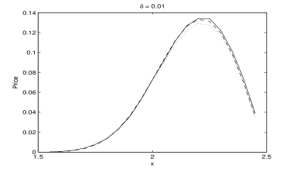
Figure 1: The price of a double-barrier call option is plotted as a function of the underlying $x$. On the left we consider the Black-Scholes model with only a fast-varying factor of volatility $Y$ whose dynamics are given by 4.20. On the right, we consider the Black-Scholes model with only a slow-varying factor of volatility $Z$ whose dynamics a given by 4.22. In each plot, the solid black line corresponds to the full price of the option, the dashed line corresponds to our approximation, and the dotted line corresponds to the Black-Scholes price. For the plots on the left we use parameters $t=1/12$, $y=0$, $r=0.05$, $\sigma=0.34$, $\rho_{xy}=-0.5$, $\beta=1$, $L=1.5$, $K=2.0$, $R=2.5$. For the plots on the right we use parameters $t=1/12$, $z=2$, $r=0.05$, $\sigma=0.34$, $\rho_{xz}=-0.5$, $g=2$, $L=1.5$, $K=2.0$, $R=2.5$.

On the left side of figure 1 we plot the approximate price $u_{0,0}+\sqrt{\epsilon}\,u_{1,0}$ of a double-barrier call option for a specific model that has only a fast-varying factor of volatility. We suppose the dynamics of $Y$ and the volatility function $f$ are given by

(4.20) $$dY_{t} =\left(-\frac{1}{\epsilon}\,Y_{t}-\frac{1}{\sqrt{\epsilon}}\beta\,\text{Erf}(Y_{t})\right)dt+\beta\,d\widetilde{W}_{t}^{y}, f(Y_{t}) =\frac{\sigma\,\exp\left(Y_{t}\right)}{\exp\left(-\beta^{2}/2\right)},$$

(4.21) $$\text{Erf}(y) :=\frac{2}{\sqrt{\pi}}\int_{0}^{y}e^{-t^{2}}dt.$$

From comparison we also plot the full price $u^{\epsilon}$ (calculated by Monte Carlo simulation) and $u_{0,0}$, which corresponds to the Black-Scholes price with volatility $\overline{\sigma}$. On the right side of figure 1 we plot the approximate price $u_{0,0}+\sqrt{\delta}\,u_{0,1}$ of a double-barrier call option for a specific model that contains only a slow-varying factor of volatility. We suppose the dynamics of $Z$ and the volatility function $f$ are given by

(4.22) $$dZ_{t} =\left(-\delta\,Z_{t}-\sqrt{\delta}\,g\,\text{Erf}(Z_{t})\right)dt+g\,d\widetilde{W}_{t}^{z}, f(Z_{t}) =\frac{\sigma\,\exp\left(Z_{t}\right)}{\exp\left(z\right)}.$$

For comparison, we also plot the full price $u^{\delta}$ (calculated by Monte Carlo simulation) and the Black-Scholes price $u_{0,0}$. As expected, as $\epsilon$ and $\delta$ go to zero, the approximate price converges to the full price, which conveges to the Black-Scholes price.

4.2 Vasicek Short-Rate with Multiscale Stochastic Volatility

In our second example, we let $X$ represent the short-rate of interest. One of the most widely known short-rate models is that of Vasicek (1977), in which $X$ is modeled as an OU process. Here, we model $X$ as an OU with multiscale stochastic volatility. Specifically, the $\widetilde{\mathbb{P}}$ dynamics of $X$ are given by

(4.23) $$dX_{t} =\Big{(}\kappa\left(\theta-X_{t}\right)-f(Y_{t},Z_{t})\Omega(Y_{t},Z_{t})\Big{)}dt+f\left(Y_{t},Z_{t}\right)\,d\widetilde{W}^{x}_{t}, r(X_{t}) =X_{t}, h(X_{t}) =0,$$

where $Y$ and $Z$ are fast- and slow-varying factors of volatility, as described in (2.6). We will calculate the approximate price of zero-coupon bond in this setting.

To start, we use equations (1.6) and (3.26) to write the operator $\left\langle\mathscr{L}_{2}\right\rangle$ and its associated speed density $\mathfrak{m}(x)$

(4.24) $$\left\langle\mathscr{L}_{2}\right\rangle =\frac{1}{2}\overline{\sigma}^{2}\partial^{2}_{xx}+\kappa\left(\overline{\theta}-x\right)\partial_{x}-x, \mathfrak{m}(x) =\frac{2}{\overline{\sigma}^{2}}\exp\left(\frac{-\kappa}{\overline{\sigma}^{2}}\left(\overline{\theta}-x\right)^{2}\right), \overline{\theta} =\theta-\tfrac{1}{\kappa}\overline{f\!\Omega}.$$

For a zero-coupon bond, the payoff at maturity is

(4.25) $$H(X_{t})\,\mathbb{I}_{\left\{\tau>t\right\}} =1.$$

In order to price a bond with payoff (4.25), we must solve eigenvalue equation (3.49) on the interval $I=(-\infty,\infty)$ with $\left\langle\mathscr{L}_{2}\right\rangle$ given by (4.24). As both $-\infty$ and $\infty$ are natural boundaries, no BCs need to be specified. The solution to this eigenvalue problem can be found in equation (4.6) of Gorovoi and Linetsky (2004)

(4.26) $$\psi_{n} =\mathscr{N}_{n}\exp\left(-A\,\xi-\frac{1}{2}A^{2}\right)H_{n}\left(\xi+A\right), \mathscr{N}_{n} =\left(\sqrt{\frac{\kappa}{\pi}}\frac{\overline{\sigma}}{2^{n+1}n!}\right)^{1/2},$$

(4.27) $$A =\frac{\overline{\sigma}}{\kappa^{3/2}}, \xi =\frac{\sqrt{\kappa}}{\overline{\sigma}}\left(x-\overline{\theta}\right),$$

(4.28) $$\lambda_{n} =\lambda_{n}=\overline{\theta}-\frac{\overline{\sigma}^{2}}{2\kappa^{2}}+\kappa\,n, n =0,1,2,\cdots.$$

Here, $\{H_{n}\}$ are the (physicists’) Hermite polynomials. Next, we use (3.34) and (3.42) to write expressions for the operators $\mathscr{A}$ and $\mathscr{B}$

(4.29) $$\mathscr{A} =-\mathscr{V}_{3}\,\partial^{3}_{xxx}-\left(\mathscr{V}_{2}+\mathscr{U}_{2}\right)\partial^{2}_{xx}-\mathscr{U}_{1}\,\partial_{x}, \mathscr{B} =-\mathscr{V}_{1}\,\partial_{x}-\mathscr{V}_{0}.$$

It is now straightforward to calculate inner products $\mathscr{A}_{k,n}$, $\mathscr{B}_{k,n}$ and $\widetilde{\mathscr{B}}_{k,n}$. Using the recursion relations

(4.30) $$\partial_{x}H_{n} =2\,nH_{n-1}, 2\,x\,H_{n} =H_{n+1}+\partial_{x}H_{n},$$

we find

(4.33) $$\mathscr{A}_{k,n} =-\mathscr{V}_{3}\left\{\sum_{m=0}^{3\wedge n}\left(\begin{array}[]{c}3\\ m\end{array}\right)\left(\frac{-1}{\kappa}\right)^{3-m}\left(\frac{2\sqrt{\kappa}}{\overline{\sigma}}\right)^{m}\frac{n!\,\mathscr{N}_{n}}{(n-m)!\,\mathscr{N}_{n-m}}\delta_{k,n-m}\right\}$$

(4.36) $$\qquad-\left(\mathscr{V}_{2}+\mathscr{U}_{2}\right)\left\{\sum_{m=0}^{2\wedge n}\left(\begin{array}[]{c}2\\ m\end{array}\right)\left(\frac{-1}{\kappa}\right)^{2-m}\left(\frac{2\sqrt{\kappa}}{\overline{\sigma}}\right)^{m}\frac{n!\,\mathscr{N}_{n}}{(n-m)!\,\mathscr{N}_{n-m}}\delta_{k,n-m}\right\}$$

(4.37) $$\qquad-\mathscr{U}_{1}\left\{\left(\frac{-1}{\kappa}\right)\delta_{k,n}+\left(\frac{2\sqrt{\kappa}}{\overline{\sigma}}\right)\frac{n!\,\mathscr{N}_{n}}{(n-1)!\mathscr{N}_{n-1}}\delta_{k,n-1}\right\},$$

(4.38) $$\mathscr{B}_{k,n} =-\mathscr{V}_{1}\left\{\left(\frac{-1}{\kappa}\right)\delta_{k,n}+\left(\frac{2\sqrt{\kappa}}{\overline{\sigma}}\right)\frac{n!\,\mathscr{N}_{n}}{(n-1)!\mathscr{N}_{n-1}}\delta_{k,n-1}\right\}-\mathscr{V}_{0}\,\delta_{k,n},$$

(4.39) $$\widetilde{\mathscr{B}}_{k,n} =-\mathscr{V}_{1}\overline{\sigma}^{\prime}\left\{\left[\left(\frac{-1}{\kappa}\right)\left(\frac{1}{2\overline{\sigma}}-\frac{\overline{\sigma}}{\kappa^{3}}-\frac{n}{\overline{\sigma}}\right)\right]\delta_{k,n}\right.$$

(4.40) $$\left.\qquad\qquad+\left[\left(\frac{-1}{\kappa}\right)\left(\frac{4}{\kappa^{3/2}}\right)+\left(\frac{2\sqrt{\kappa}}{\overline{\sigma}}\right)\left(\frac{1}{2\overline{\sigma}}-\frac{\overline{\sigma}}{\kappa^{3}}-\frac{n}{\overline{\sigma}}\right)\right]\frac{n!\mathscr{N}_{n}}{(n-1)!\mathscr{N}_{n-1}}\delta_{k,n-1}\right.$$

(4.41) $$\left.\qquad\qquad+\left[\left(\frac{-1}{\kappa}\right)\left(\frac{-2}{\overline{\sigma}}\right)+\left(\frac{2\sqrt{\kappa}}{\overline{\sigma}}\right)\left(\frac{4}{\kappa^{3/2}}\right)\right]\frac{n!\mathscr{N}_{n}}{(n-2)!\mathscr{N}_{n-2}}\delta_{k,n-2}\right.$$

(4.42) $$\left.\qquad\qquad+\left[\left(\frac{2\sqrt{\kappa}}{\overline{\sigma}}\right)\left(\frac{-2}{\overline{\sigma}}\right)\right]\frac{n!\mathscr{N}_{n}}{(n-3)!\mathscr{N}_{n-3}}\delta_{k,n-3}\right\}$$

(4.43) $$\qquad-\mathscr{V}_{0}\overline{\sigma}^{\prime}\left\{\left(\frac{1}{2\overline{\sigma}}-\frac{\overline{\sigma}}{\kappa^{3}}-\frac{n}{\overline{\sigma}}\right)\delta_{k,n}+\left(\frac{4}{\kappa^{3/2}}\right)\frac{n!\,\mathscr{N}_{n}}{(n-1)!\mathscr{N}_{n-1}}\delta_{k,n-1}\right.$$

(4.44) $$\left.\qquad\qquad+\left(\frac{-2}{\overline{\sigma}}\right)\frac{n!\mathscr{N}_{n}}{(n-2)!\mathscr{N}_{n-2}}\delta_{k,n-2}\right\}$$

(4.45) $$\qquad-\mathscr{V}_{1}\overline{f\!\Omega}^{\prime}\left\{\left(\frac{1}{\kappa^{3}}\right)\delta_{k,n}+\left(\frac{-4}{\overline{\sigma}\kappa^{3/2}}\right)\frac{n!\mathscr{N}_{n}}{(n-1)!\mathscr{N}_{n-1}}\delta_{k,n-1}+\left(\frac{4}{\overline{\sigma}^{2}}\right)\frac{n!\mathscr{N}_{n}}{(n-2)!\mathscr{N}_{n-2}}\delta_{k,n-2}\right\}$$

(4.46) $$\qquad-\mathscr{V}_{0}\overline{f\!\Omega}^{\prime}\left\{\left(\frac{-1}{\kappa^{2}}\right)\delta_{k,n}+\left(\frac{2}{\overline{\sigma}\sqrt{\kappa}}\right)\frac{n!\mathscr{N}_{n}}{(n-1)!\mathscr{N}_{n-1}}\delta_{k,n-1}\right\}.$$

The computation of $c_{n}$ be found on page 63 of in Gorovoi and Linetsky (2004)

(4.47) $$c_{n} =\left(\psi_{n},1\right)=\frac{2}{\overline{\sigma}}\sqrt{\frac{\pi}{\kappa}}\mathscr{N}_{n}A^{n}e^{-A^{2}/4}.$$

The approximate price of a bond can now be calculated using Theorems 3.1, 3.2 and 3.3.

Yield Curve

For a zero-coupon bond, it is often the yield curve, rather than the bond price itself, that is of fundamental importance. The yield $R^{\epsilon,\delta}$ of a zero-coupon bond that pays one dollar at time $t$ is defined via the relation

(4.48) $$u^{\epsilon,\delta} =\exp\left(-R^{\epsilon,\delta}t\right).$$

We can obtain an approximation for the yield of a zero-coupon bond by expanding both the bond price $u^{\epsilon,\delta}$ and yield $R^{\epsilon,\delta}$ in powers of $\sqrt{\epsilon}$ and $\sqrt{\delta}$ as follows

(4.49) $$u_{0,0}+\sqrt{\epsilon}\,u_{1,0}+\sqrt{\delta}\,u_{0,1}+\cdots =e^{-\left(R_{0,0}+\sqrt{\epsilon}\,R_{1,0}+\sqrt{\delta}\,R_{0,1}+\cdots\right)\,t}$$

(4.50) $$=e^{-R_{0,0}t}+\sqrt{\epsilon}\left(-R_{1,0}\,t\right)e^{-R_{0,0}t}+\sqrt{\delta}\left(-R_{0,1}\,t\right)e^{-R_{0,0}t}+\cdots.$$

Matching terms of like-powers of $\sqrt{\epsilon}$ and $\sqrt{\delta}$ we obtain

(4.51) $$R^{\epsilon,\delta} \approx R_{0,0}+\sqrt{\epsilon}\,R_{1,0}+\sqrt{\delta}\,R_{0,1},$$

(4.52) $$R_{0,0} =-\tfrac{1}{t}\log\left(u_{0,0}\right),\qquad R_{1,0}=\frac{-u_{1,0}}{t\,u_{0,0}},\qquad R_{0,1}=\frac{-u_{0,1}}{t\,u_{0,0}},$$

On the left side of figure 2 we plot the approximate yield $R_{0,0}+\sqrt{\epsilon}\,R_{1,0}$ of a zero coupon bond for a specific model that has only a fast-varying factor of volatility. We suppose the dynamics of $Y$ and the volatility function $f$ are given by (4.20). For comparison, we also plot the full yield $R^{\epsilon}$ (calculated by Monte Carlo simulation) and the Vasicek yield $R_{0,0}$. On the right side of figure 2 we plot the approximate yield $R_{0,0}+\sqrt{\delta}\,R_{0,1}$ of a zero coupon bond for a specific model that has only a slow-varying factor of volatility. We suppose the dynamics of $Z$ and the volatility function $f$ are given by (4.22). For comparison, we also plot the full yield $R^{\delta}$ (calculated by Monte Carlo simulation) and the Vasicek yield $R_{0,0}$. As expected, as $\epsilon$ and $\delta$ go to zero, the approximate yield converges to the full yield, which converges to the Vasicek yield.

4.3 Jump to Default CEV with Multiscale Stochastic Volatility

In our final example, we consider a non-dividend-paying, defaultable asset $S_{t}=\mathbb{I}_{\{\tau>t\}}X_{t}$. As $S$ must be non-negative, we let the state space of $X$ be $(e_{1},e_{2})=(0,\infty)$. We base our multiscale diffusion on the jump to default constant elastic variance model (JDCEV) of Carr and Linetsky (2006). Specifically, the $\widetilde{\mathbb{P}}$ dynamics of $X$ prior to default are given by

(4.53) $$dX_{t} =\left(\mu+c\,X_{t}^{2\eta}\right)X_{t}\,dt+\left(f(Y_{t},Z_{t})\,X_{t}^{\eta}\right)X_{t}\,d\widetilde{W}_{t}^{x}, h(X_{t}) =\mu+c\,X_{t}^{2\eta}.$$

For computational convenience we have set the risk-free interest rate to zero: $r=0$. The constants $\mu$ and $c$ are assumed to be strictly positive. As always, $Y$ and $Z$ are fast- and slow-varying factors of volatility, as described in (2.6). Note that the volatility of $X$ has both a local component $X_{t}^{\eta}$ and a nonlocal multiscale component $f(Y_{t},Z_{t})$. We assume $\eta<0$ so that the local component of volatility $X_{t}^{\eta}$ increases as $X_{t}$ decreases, reflecting the fact that price and volatility are negatively correlated. The stochastic hazard rate $h(X_{t})$ also increases as $X$ decreases, capturing the idea that the probability of default increases as $X$ tends to zero. Note that $S$ is a $\widetilde{\mathbb{P}}$-martingale, as it should be. We will calculate the approximate price of a European put option written on $S$. The price of a European call option can be obtained through put-call parity.

To begin, we use (1.6) and (3.26) to write the operator $\left\langle\mathscr{L}_{2}\right\rangle$ and its associated speed density $\mathfrak{m}(x)$

(4.54) $$\left\langle\mathscr{L}_{2}\right\rangle =\frac{1}{2}\overline{\sigma}^{2}x^{2\eta+2}\partial^{2}_{xx}+\left(\mu+c\,x^{2\eta}\right)x\,\partial_{x}-\left(\mu+c\,x^{2\eta}\right),$$

(4.55) $$\mathfrak{m}(x) =\frac{2}{\overline{\sigma}^{2}}x^{2c/\overline{\sigma}^{2}-2-2\eta}\exp\left(A\,x^{-2\eta}\right), A =\frac{\mu}{\overline{\sigma}^{2}|\eta|}$$

For the diffusion associated with infinitesimal generator (4.54) the endpoint $e_{2}=\infty$ is a natural boundary. However, the classification of endpoint $e_{1}=0$ depends on the values of $\eta$ and $c/\overline{\sigma}^{2}$. The classification is as follows

(4.56) $$c/\overline{\sigma}^{2} \geq 1/2 \eta <0, e_{1}=0$$ and is natural,

(4.57) $$c/\overline{\sigma}^{2} \in(0,1/2) \eta \in[c/\overline{\sigma}^{2}-1/2,0), e_{1}=0$$ and is exit,

(4.58) $$c/\overline{\sigma}^{2} \in(0,1/2) \eta <c/\overline{\sigma}^{2}-1/2, e_{1}=0$$ and is regular.

If the parameters ($c$, $\overline{\sigma}$, $\eta$) are chosen such that $e_{1}=0$ is regular, then we specify $e_{1}=0$ as a killing boundary. To calculate the approximate price of a European put we must solve the eigenvalue equation (3.49) on the interval $(0,\infty)$ with $\left\langle\mathscr{L}_{2}\right\rangle$ given by (4.54) and with the BC

(4.59) $$\lim_{x\searrow 0}\psi_{n}(x) =0, c/\overline{\sigma}^{2} \in(0,1/2).$$ if

The solution is given in equation (8.11) of Theorem 8.2 in Mendoza-Arriaga, Carr, and Linetsky (2010)

(4.60) $$\psi_{n} =A^{\nu/2}\sqrt{\frac{(n-1)!\,\mu}{\Gamma(\nu+n)}}\,x\,\exp\left(-A\,x^{-2\eta}\right)L_{n-1}^{(\nu)}\left(A\,x^{-2\eta}\right), n =1,2,3,\cdots,$$

(4.61) $$\lambda_{n} =2\mu|\eta|(n+\nu), \nu =\frac{1+2\,(c/\overline{\sigma}^{2})}{2|\eta|},$$

where $\{L_{n}^{(\nu)}\}$ are the generalized Laguerre polynomials. Next, we use (3.34) and (3.42) to write expressions for the operators $\mathscr{A}$ and $\mathscr{B}$

(4.62) $$\mathscr{A} =-\mathscr{V}_{3}\,x^{\eta+1}\partial_{x}x^{2\eta+2}\partial^{2}_{xx}-\mathscr{V}_{2}\,x^{2\eta+2}\partial^{2}_{xx}, \mathscr{B} =-\mathscr{V}_{1}\,x^{\eta+1}\partial_{x}-\mathscr{V}_{0}.$$

Analytic expressions for $\mathscr{A}_{k,n}$, $\mathscr{B}_{k,n}$ and $\widetilde{\mathscr{B}}_{k,n}$ are easily derived by making the change of variables $A\,x^{-2\eta}\to y$, using $\partial_{y}L_{n}^{\nu}(y)=-L_{n-1}^{(\nu+1)}(y)$ and

(4.63) $$\int_{0}^{\infty}y^{\gamma}e^{-y}L_{n}^{(\alpha)}(y)L_{m}^{(\beta)}(y)\,dy$$

(4.66) $$\qquad=\frac{\Gamma(\alpha-\gamma+n)\Gamma(\beta+1+m)\Gamma(\gamma+1)}{\Gamma(\alpha-\gamma)\Gamma(\beta+1)\,n!\,m!}\,{}_{3}F_{2}\left(\begin{array}[]{ccc}\gamma+1,&-m,&\gamma+1-\alpha\\ \beta+1,&\gamma+1-\alpha-n,&\end{array};1\right),$$

where where ${}_{p}F_{q}$ is a generalized hypergeometric function (the above formula is given in equation (14) of Shawagfeh (2011)). As the formulas for $\mathscr{A}_{k,n}$, $\mathscr{B}_{k,n}$ and $\widetilde{\mathscr{B}}_{k,n}$ are quite long, for the sake of brevity, we do not provide them here.

The payoff of a European put option with strike price $K>0$ can be decomposed as follows

(4.67) $$(K-S_{t})^{+} =(K-X_{t})^{+}\,\mathbb{I}_{\left\{\tau>t\right\}}+K\left(1-\mathbb{I}_{\left\{\tau>t\right\}}\right).$$

The first term on the RHS of (4.67) represents the payoff of a put given no default prior to time $t$. The second term represents the payoff of a put option given a default occurs prior to time $t$. Thus, the value of a put option with strike price $K$ – denoted $u^{\epsilon,\delta}(t,x;K)$ – can be expressed as the sum of two parts

(4.68) $$u^{\epsilon,\delta}(t,x;K) =u_{0}^{\epsilon,\delta}(t,x;K)+u_{D}^{\epsilon,\delta}(t,x;K),$$

where

(4.69) $$u_{0}^{\epsilon,\delta}(t,x;K) =\widetilde{\mathbb{E}}_{x,y,z}\left[(K-X_{t})^{+}\mathbb{I}_{\left\{\tau>t\right\}}\right],$$

(4.70) $$u_{D}^{\epsilon,\delta}(t,x;K) =K-K\,\widetilde{\mathbb{E}}_{x,y,z}\left[\mathbb{I}_{\left\{\tau>t\right\}}\right]$$

(4.71) $$=K-K\int_{0}^{\infty}\widetilde{\mathbb{E}}_{x,y,z}\left[\delta_{x^{\prime}}(X_{t})\,\mathbb{I}_{\left\{\tau>t\right\}}\right]dx^{\prime}$$

(4.72) $$=K-K\,\int_{0}^{\infty}u_{1}^{\epsilon,\delta}(t,x;x^{\prime})\,dx^{\prime},$$

(4.73) $$u_{1}^{\epsilon,\delta}(t,x;x^{\prime}) =\widetilde{\mathbb{E}}_{x,y,z}\left[\delta_{x^{\prime}}(X_{t})\,\mathbb{I}_{\left\{\tau>t\right\}}\right].$$

Note, because $1\notin L^{2}(\mathbb{R}^{+},\mathfrak{m})$, we have used the fact that $1=\int_{0}^{\infty}\delta_{x^{\prime}}(X_{t})\,dx^{\prime}$ on the set $\left\{\tau>t\right\}$. This substitution comes at a cost; the integral in (4.72) must be computed numerically. However, numerical evaluation of (4.72) is not computationally intensive and does not pose any major difficulties.

Since the payoff functions $H_{0}(x)=(K-x)^{+}$ and $H_{1}(x)=\delta_{x^{\prime}}(x)$ belong to $L^{2}(\mathbb{R}^{+},\mathfrak{m})$, we may calculate

(4.74) $$c_{0,n} =\left(\psi_{n}(\cdot),(k-\cdot)^{+}\right), c_{1,n} =\left(\psi_{n},\delta_{x^{\prime}}\right).$$

The expression for $c_{0,n}$ can be found in equation (8.15) of Theorem 8.4 in Mendoza-Arriaga, Carr, and Linetsky (2010). The expression for $c_{1,n}$ is computed trivially. We have

(4.75) $$c_{0,n} =\frac{A^{\nu/2+1}K^{2c/\overline{\sigma}^{2}+1-2\eta}\sqrt{\Gamma(\nu+n)}}{\Gamma(\nu+1)\sqrt{\mu(n-1)!}}\,\times$$

(4.78) $$\qquad\left[\frac{|\eta|}{(c/\overline{\sigma}^{2})+|\eta|}\,{}_{2}F_{2}\left(\begin{array}[]{cc}1-n,&\tfrac{c/\overline{\sigma}^{2}}{|\eta|}+1\\ \nu+1,&\tfrac{c/\overline{\sigma}^{2}}{|\eta|}+2\end{array};A\,K^{-2\eta}\right)-\frac{\Gamma(\nu+1)(n-1)!}{\Gamma(\nu+n+1)}L_{n-1}^{(\nu+1)}(A\,K^{-2\eta})\right],$$

(4.79) $$c_{1,n} =\psi_{n}(x^{\prime})\,\mathfrak{m}(x^{\prime}).$$

The approximate price of a European put option can now be computed using Theorems 3.1, 3.2 and 3.3.

For European options, it is often the implied volatility induced by an option price, rather than the option price itself that is of primary interest. Recall that the implied volatility $I^{\epsilon,\delta}$ of a put option with price $u^{\epsilon,\delta}(t,x;K)$ is defined implicitly through

(4.80) $$u^{\epsilon,\delta}(t,x;K)=u^{\text{BS}}(t,x,I^{\epsilon,\delta};K)$$

where $u^{\text{BS}}(t,x,I^{\epsilon,\delta};K)$ is the Black-Scholes price of a put as calculated with volatility $I^{\epsilon,\delta}$.

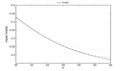
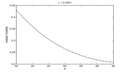
Figure 3: The implied volatility of a European put option is plotted as a function of the strike price $K$. On the left we consider a JDCEV model with only a fast-varying factor of volatility $Y$ whose dynamics are given by 4.20. On the right, we consider the JDCEV model with only a slow-varying factor of volatility $Z$ whose dynamics a given by 4.22. In each plot, the solid black line corresponds to the full implied volatility, the dashed line corresponds to our approximation, and the dotted line corresponds to the JDCEV implied volatility. For the plots on the left we use parameters $t=1$, $x=50$, $\mu=0.05$, $\sigma=10$, $\eta=-1$, $c=0.5$, $\rho_{xy}=-0.5$, $y=0$ and $\beta=2$. For the plots on the right we use parameters $t=1$, $x=50$, $\mu=0.05$, $\sigma=10$, $\eta=-1$, $c=0.5$, $\rho_{xz}=-0.5$, $z=2$ and $g=2$.

On the left side of figure 3 we plot the implied volatility induced by the approximate price $u_{0,0}+\sqrt{\epsilon}\,u_{1,0}$ of a put option for a specific model that has only a fast-varying factor of volatility. We suppose the dynamics of $Y$ and the volatility function $f$ are given by (4.20). For comparison, we also plot the implied volatility induced by the full price $u^{\epsilon}$ (calculated by Monte Carlo simulation) and the implied volatility induced by the JDCEV price $u_{0,0}$. On the right side of figure 3 we plot the implied volatility induced by the approximate price $u_{0,0}+\sqrt{\delta}\,u_{0,1}$ of a put option for a specific model that has only a slow-varying factor of volatility. We suppose the dynamics of $Z$ and the volatility function $f$ are given by (4.22). For comparison, we also plot the implied volatility induced by the full price $u^{\delta}$ (calculated by Monte Carlo simulation) and the implied volatility induced by the JDCEV price $u_{0,0}$. As expected, as $\epsilon$ and $\delta$ go to zero, the implied volatility induced by the approximate price converges to the implied volatility induced by the full price, which converges to the implied volatility induced by the JDCEV price.

5 Review and Conclusions

This paper develops a general method for obtaining the approximate price for a large class of derivative-assets. The payoff of the derivatives may be path-dependent and the process underlying the derivative-assets may exhibit jump to default as well as combined local/nonlocal stochastic volatility. The intensity of the jump to default event may be state-dependent and the nonlocal component of volatility may be multiscale, driven by one fast-varying and one slow-varying factor.

One key advantage of our pricing methodology is that, by combining techniques from spectral theory, singular perturbation theory and regular perturbation theory, we reduce the derivative pricing problem to that of solving a single eigenvalue equation. Once this equation is solved, the approximate price of a derivative-asset may be calculated formulaically. We have illustrated the simplicity and flexibility of our method by calculating the approximate prices of thre derivative assets: a double-barrier option on a non-defaultable stock, a European option on a defaultable stock, and a non-defaultable bond in a short-rate model.

We believe that the flexibility of our framework, as well as the analytic tractability that our pricing methodology provides merit further research in this area. A logical next step, for example, would be to extend the results of this paper to include cases where the eigenvalue equation (3.49) does not have a purely discrete spectrum.

Thanks

The authors of this paper would like to thank Stephan Sturm, Ronnie Sircar and Jean-Pierre Fouque for helpful conversations. Additionally, the authors would like to thank two anonymous referees, whose comments vastly improved both the quality and readability of this manuscript.

Appendix A Appendix

A.1 Self-Adjoint Operators acting on a Hilbert Space

In this appendix we summarize some basic properties of self-adjoint operators acting on a Hilbert space. A detailed exposition on this topic (including proofs) can be found in Reed and Simon (1980). We shall closely follow Linetsky (2007), who provides a more streamlined review.

Let $\mathscr{H}$ be a real, separable Hilbert space with inner product $(\cdot,\cdot)$. A linear operator is a pair $(\text{dom}(\mathscr{L}),\mathscr{L})$ where $\text{dom}(\mathscr{L})$ is a linear subset of $\mathscr{H}$ and $\mathscr{L}$ is a linear map $\mathscr{L}:\text{dom}(\mathscr{L})\to\mathscr{H}$. The adjoint of an operator $\mathscr{L}$ is an operator $\mathscr{L}^{*}$ such that $(\mathscr{L}f,g)=(f,\mathscr{L}^{*}g),\forall\,f\in\text{dom}(\mathscr{L}),g\in\text{dom}(\mathscr{L}^{*})$, where

(A.1) $$\text{dom}(\mathscr{L}^{*}):=\{g\in\mathscr{H}:\exists\,h\in\mathscr{H}\text{ such that }(\mathscr{L}f,g)=(f,h)\,\,\forall\,f\in\text{dom}(\mathscr{L})\}.$$

An operator $(\text{dom}(\mathscr{L}),\mathscr{L})$ is said to be self-adjoint in $\mathscr{H}$ if

(A.2) $$\text{dom}{(\mathscr{L})} =\text{dom}(\mathscr{L}^{*}), (\mathscr{L}f,g) =(f,\mathscr{L}g) \forall\,f,g\in\text{dom}(\mathscr{L}).$$

Throughout this appendix, for any self-adjoint operator $\mathscr{L}$, we will assume that $\text{dom}(\mathscr{L})$ is a dense subset of $\mathscr{H}$.

Given a linear operator $\mathscr{L}$, the resolvent set $\rho(\mathscr{L})$ is defined as the set of $\lambda\in\mathbb{C}$ such that the mapping $(\mathscr{L}-\text{Id}\,\lambda)$ is one-to-one and $R_{\lambda}:=(\mathscr{L}-\text{Id}\,\lambda)^{-1}$ is continuous with $\text{dom}(R_{\lambda})=\mathscr{H}$. The operator $R_{\lambda}:\mathscr{H}\to\mathscr{H}$ is called the resolvent. The spectrum $\sigma(\mathscr{L})$ of an operator $\mathscr{L}$ is defined as $\sigma(\mathscr{L}):=\mathbb{C}\setminus\rho(\mathscr{L})$. If $\mathscr{L}$ is self-adjoint, its spectrum is non-empty and real. We say that $\lambda\in\sigma(\mathscr{L})$ is an eigenvalue of $\mathscr{L}$ if there exists $\psi\in\text{dom}(\mathscr{L})$ such that the eigenvalue equation is satisfied

(A.3) $$\mathscr{L}\,\psi =\lambda\,\psi.$$

A function $\psi$ that solves (A.3) is called an eigenfunction of $\mathscr{L}$ corresponding to $\lambda$. The multiplicity of an eigenvalue $\lambda$ is the number of linearly independent eigenfunctions for which equation (A.3) is satisfied. The spectrum of an operator $\mathscr{L}$ can be decomposed into two disjoint sets called the discrete and essential spectrum $\sigma(\mathscr{L})=\sigma_{d}(\mathscr{L})\cup\sigma_{e}(\mathscr{L})$. For a self-adjoint operator $\mathscr{L}$, a number $\lambda\in\mathbb{R}$ belongs to $\sigma_{d}(\mathscr{L})$ if and only if $\lambda$ is an isolated point of $\sigma(\mathscr{L})$ and $\lambda$ is an eigenvalue of finite multiplicity.

The spectral representation Theorem is an important tool for analysing self-adjoint operators acting on a Hilbert space. We state this theorem below in a form which is convenient for the computations in this paper.

Theorem A.1.

Assume $\mathscr{L}$ is a self-adjoint operator in $\mathscr{H}$ and assume $\mathscr{L}$ has a purely discrete spectrum (i.e., $\sigma_{e}(\mathscr{L})=\{\emptyset\}$). The Spectral Representation Theorem states that $\mathscr{L}f$ has an eigenfunction expansion

(A.4) $$\mathscr{L}f =\sum_{n}\lambda_{n}\,(\psi_{n},f)\,\psi_{n}, \forall\,f \in\text{\emph{dom}}(\mathscr{L}),$$

where the sum runs over all solutions $\{\lambda_{n},\psi_{n}\}$ of the eigenvalue equation (A.3). Furthermore, for any real-valued Borel-measurable function on $\mathbb{R}$ one can define an operator $\phi(\mathscr{L})$ using functional calculus

(A.5) $$\phi(\mathscr{L})f :=\sum_{n}\phi(\lambda_{n})\,(\psi_{n},f)\,\psi_{n}, \forall\,f \in\text{\emph{dom}}(\phi(\mathscr{L})),$$

(A.6) $$\text{\emph{dom}}(\phi(\mathscr{L})) :=\{f\in\text{\emph{dom}}(\mathscr{L}):\sum_{n}\phi^{2}(\lambda_{n})\left(\psi_{n},f\right)^{2}<\infty\}.$$

The operator $\phi(\mathscr{L})$ is self-adjoint in $\mathscr{H}$ and $\text{\emph{dom}}(\phi(\mathscr{L}))\subseteq\text{\emph{dom}}(\mathscr{L})$.

Proof.

See Reed and Simon (1980) Theorem VIII.6. ∎

Note that setting $\phi(\lambda)=\text{Id}$ yields

(A.7) $$\text{Id}\,f =\sum_{n}(\psi_{n},f)\,\psi_{n}, \forall\,f \in\mathscr{H},$$

which is equivalent to saying that the eigenfunctions $\{\psi_{n}\}$ of a densely defined self-adjoint operator in $\mathscr{H}$ form a Schauder basis. In fact, the basis can be chosen to be orthonormal $(\psi_{n},\psi_{m})=\delta_{n,m}$. Also note, setting $\phi(\lambda)=R_{\lambda}$ yields an eigenfunction representation of the resolvent operator

(A.8) $$R_{\lambda}\,f =\sum_{n}\frac{(\psi_{n},f)}{\lambda_{n}-\lambda}\,\psi_{n}, \forall\,f \in\mathscr{H},\,\lambda\in\rho(\mathscr{L}).$$

A.2 Boundary Conditions

According to Feller (1954), the endpoints $e_{1}$ and $e_{2}$ of a one-dimensional diffusion in an interval $I$ can be classified as either natural, exit, entrance or regular. The classification, which can be found in Borodin and Salminen (2002); Linetsky (2007), is done as follows. For a general infinitesimal generator $\mathscr{L}$ of the form (1.5) one can associate a scale density

(A.9) $$\mathfrak{s}(x) :=\exp\left(-\int_{x_{0}}^{x}\frac{2b(y)}{a^{2}(y)}dy\right), (\text{scale density)}$$

where the lower limit of integration $x_{0}\in(e_{1},e_{2})$ may be chosen arbitrarily. From $\mathfrak{s}$ one can define a scale function $\mathscr{S}$

(A.10) $$\mathscr{S}\left(\left[x,y\right]\right) :=\int_{x}^{y}\mathfrak{s}(z)\,dz, x,y \in\left(e_{1},e_{2}\right),$$

(A.11) $$\mathscr{S}\left(\left(e_{1},y\right]\right) :=\lim_{x\searrow e_{1}}\mathscr{S}\left(\left[x,y\right]\right), \mathscr{S}\left(\left[x,e_{2}\right)\right) :=\lim_{y\nearrow e_{2}}\mathscr{S}\left(\left[x,y\right]\right).$$

Note that the above limits may be infinite. For some arbitrary $y\in\left(e_{1},e_{2}\right)$ we define

(A.12) $$I_{1} :=\int_{e_{1}}^{y}\mathscr{S}\left(\left(e_{1},x\right]\right)\left(1+k(x)\right)\mathfrak{m}(x)\,dx, I_{2} :=\int_{y}^{e_{2}}\mathscr{S}\left(\left[x,e_{2}\right)\right)\left(1+k(x)\right)\mathfrak{m}(x)\,dx,$$

(A.13) $$J_{1} :=\int_{e_{1}}^{y}\mathscr{S}\left(\left[x,y\right]\right)\left(1+k(x)\right)\mathfrak{m}(x)\,dx, J_{2} :=\int_{y}^{e_{2}}\mathscr{S}\left(\left[y,x\right]\right)\left(1+k(x)\right)\mathfrak{m}(x)\,dx.$$

An endpoint $e_{i}$ is classified as

• Natural if $I_{i}=\infty$ and $J_{i}=\infty$. No BC needs to be specified at a natural boundary. The interval $I$ is taken to be open at a natural boundary.

• Exit if $I_{i}<\infty$ and $J_{i}=\infty$. The appropriate BC at an exit boundary is

  (A.14) $$\lim_{x\rightarrow e_{i}}\psi(x) =0.$$

  The interval $I$ is taken to be open at an exit boundary.

• Entrance if $I_{i}=\infty$ and $J_{i}<\infty$. The appropriate BC at an entrance boundary is

  (A.15) $$\lim_{x\rightarrow e_{i}}\frac{\partial_{x}\psi(x)}{\mathfrak{s}(x)} =0.$$

  The interval $I$ is taken to be open at an entrance boundary.

• Regular if $I_{i}<\infty$ and $J_{i}<\infty$. We must specify the behavior of a diffusion at a regular boundary. Here, we consider only killing and instantaneously reflecting behavior, for which the appropriate BCs are

  (A.16) $$\lim_{x\rightarrow e_{i}}\psi(x) =0\qquad\text{(killing BC)}, \lim_{x\rightarrow e_{i}}\frac{\partial_{x}\psi(x)}{\mathfrak{s}(x)} =0\qquad\text{(instantaneously reflecting BC)}$$

  The interval $I$ is taken to be open at a regular boundary specified as a killing boundary and closed at a regular boundary specified as instantaneously reflecting.

The domain of $\mathscr{L}$ is then

(A.17) $$\text{Dom}\left(\mathscr{L}\right) =\left\{f\in L^{2}\left(I,\mathfrak{m}\right):f,\partial_{x}f\in AC_{\text{loc}}(I),\mathscr{L}f\in L^{2}\left(I,\mathfrak{m}\right),\text{BCs at $e_{1}$ and $e_{2}$}\right\},$$

where $AC_{\text{loc}}(I)$ is the space of functions that are absolutely continuous over each compact subinterval of $I$ (see Linetsky (2007), p. 242). The BCs at $e_{1}$ and $e_{2}$ correspond to the BCs specified above for natural, exit, entrance and regular boundaries.

A.3 Specific Model Assumptions

1. We assume existence and uniqueness of $(X,Y,Z)$ as the strong solution to (2.2).

2. We assume existence and uniqueness of $(X,Y,Z)$ as the strong solution to (2.6).

3. There exist positive constants $C_{\Lambda}<\infty$ and $C_{\Gamma}<\infty$ such that $||\Lambda||_{\infty}<C_{\Lambda}$ and $||\Gamma||_{\infty}<C_{\Gamma}$.

4. Define the time-rescaled process $Y^{(1)}_{t}:=Y_{\epsilon\,t}$. Under $\mathbb{P}$, the process $Y^{(1)}$ has infinitesimal generator $\mathscr{L}_{0}$. Under $\mathbb{P}$ we assume:

   1. The process $Y^{(1)}$ is ergodic and has a unique invariant distribution $\Pi$ with density $\pi$.

   2. The operator $\mathscr{L}_{0}$ has a strictly positive spectral gap – meaning the smallest non-zero eigenvalue $\lambda_{min}$ of $\left(-\mathscr{L}_{0}\right)$ is strictly positive.

   3. The process $Y^{(1)}$ is reversible – meaning $\mathscr{L}_{0}$ is self-adjoint acting on $L^{2}\left(\mathbb{R},\pi\right)$.

   These assumptions guarantee (see Fouque, Papanicolaou, Sircar, and Solna (2011), p. 93) exponential convergence of $Y^{(1)}$ to its invariant distribution

   (A.18) $$\left|\mathbb{E}\left[g\left(Y_{t}^{(1)}\right)\right]-\left\langle g\right\rangle\right| \leq C\,\exp\left(-\lambda_{min}t\right), \forall\,g \in L^{2}\left(\mathbb{R},\pi\right).$$

   The above assumptions also ensure (see Fouque, Papanicolaou, Sircar, and Solna (2011), p. 139) that for all $k\in\mathbb{N}$ there exists $C(k)<\infty$ such that

   (A.19) $$\sup_{t}\mathbb{E}\left[\left|Y_{t}^{(1)}\right|^{k}\right] \leq C(k).$$

5. Define the time-rescaled process $Z^{(1)}_{t}:=Z_{t/\delta}$. Under $\mathbb{P}$, the process $Z^{(1)}$ has infinitesimal generator $\mathscr{M}_{2}$. Under $\mathbb{P}$ we assume the process $Z^{(1)}$ admits moments that are uniformly bounded in $s<t$. That is, for all $k\in\mathbb{N}$ there exists $C(t,k)<\infty$ such that

   (A.20) $$\sup_{s\leq t}\mathbb{E}\left[\left|Z_{s}^{(1)}\right|^{k}\right] \leq C(t,k).$$

6. We assume that the functions $f(y,z)$ and $\Omega(y,z)$ satisfy $\overline{\sigma}^{2}(z)<\infty$, $\overline{f\!\Omega}(z)<\infty$ and the solutions $\phi(y,z)$ and $\eta(y,z)$ to Poisson equations (3.31) are at most polynomially growing.

7. The functions $a(x)$ $b(x)$, $r(x)$ and $h(x)$ satisfy $a>0$, $a\in C^{2}(I)$, $b\in C^{1}(I)$, $r\geq 0$, $r\in C(I)$, $h\geq 0$, and $h\in C(I)$.

8. The spectrum of the operator $\left\langle\mathscr{L}_{2}\right\rangle$, defined in (3.26), is simple and purely discrete.

We note that two of the processes that are most commonly used to model volatility – the Cox-Ingersoll-Ross (CIR) and Ornstein-Uhlenbeck (OU) processes – satisfy the assumptions placed on both $Y^{(1)}$ and $Z^{(1)}$.

A.4 Poisson Equations and the Fredholm Alternative

In this appendix we review the existence and uniqueness of solutions to Poisson equations. Central to this discussion will be a statement of the Fredholm alternative. Our presentation follows page 93 of Fouque, Papanicolaou, Sircar, and Solna (2011), as well as page 124 of Fouque, Garnier, Papanicolaou, and Sølna (2007).

Let $\mathscr{L}$ be a self-adjoint operator densely defined on a real separable Hilbert space $\mathscr{H}$, and let $\{\psi_{n},\lambda_{n}\}$ be the complete set of solutions to eigenvalue equation $\mathscr{L}\psi_{n}=\lambda_{n}\psi_{n}$. Consider the following Poisson problem: find, $\psi\in\mathscr{H}$ such that

(A.21) $$\left(\mathscr{L}-\lambda\right)\psi =\chi,$$

where the function $\chi\in\mathscr{H}$ and the constant $\lambda$ are given.

Theorem A.2.

The Fredholm Alternative states that one of the following is true:

1. Either $\lambda$ is not an eigenvalue of $\mathscr{L}$, in which case equation (A.21) has a unique solution

   (A.22) $$\psi =R_{\lambda}\,\chi=\sum_{n}\frac{(\psi_{n},\chi)}{\lambda_{n}-\lambda}\,\psi_{n}.$$

2. Or, $\lambda$ is an eigenvalue of $\mathscr{L}$. Suppose this is the case. Let $\lambda=\lambda_{1}=\lambda_{2}=\cdots=\lambda_{m}$ (i.e., the eigenvalue $\lambda$ has multiplicity $m$). Then (A.21) has a solution if and only if $\left(\psi_{n},\chi\right)=0$ for all $n\leq m$. Assuming $\left(\psi_{n},\chi\right)=0$ for all $n\leq m$, a solution to (A.21) has the form

   (A.23) $$\psi =\sum_{n>m}\frac{(\psi_{n},\chi)}{\lambda_{n}-\lambda_{k}}\,\psi_{n}+\sum_{n\leq m}c_{n}\psi_{n}, c_{n} \in\mathbb{R}.$$

Proof.

See Reed and Simon (1980), Theorem VI.14 and the ensuing corollary. ∎

Classically, the Fredholm alternative Theorem holds for compact operators on a Hilbert space. However, the Theorem also holds true for differential operators $\mathscr{L}$ of the form (1.5), with domain (A.17) acting on the Hilbert space $\mathscr{H}=L^{2}(I,\mathfrak{m})$, where $\mathfrak{m}$ is the speed density corresponding to $\mathscr{L}$ (see section 9.4.2 of Haberman (2004)).

In particular, we note that $\lambda=0$ is an eigenvalue of $\mathscr{L}_{0}$, which is a self-adjoint operator in $L^{2}(\mathbb{R},\pi)$. The corresponding (normalized) eigenfunction is the constant $\psi_{\lambda}=1$. Thus, in order for $\mathscr{L}_{0}u=\chi$ to have a solution $u\in L^{2}(\mathbb{R},\pi)$ we must have $\left(1,\chi\right)=\int\chi\pi dy=:\left\langle\chi\right\rangle=0$, which is the centering condition (3.23).

A.5 Proof of Theorem 3.2

We must show that $u_{1,0}$, given by (3.53) satisfies PDE and BC (3.45). It is obvious that the BC $u_{1,0}(0,x,z)=0$ is satisfied. To show that $u_{1,0}$ satisfies PDE (3.45) we note that

(A.24) $$\mathscr{A}u_{0,0} =\sum_{n}c_{n}\left(\mathscr{A}\psi_{n}\right)T_{n}=\sum_{n}\sum_{k}c_{n}\mathscr{A}_{k,n}\psi_{k}T_{n},$$

where we have used (A.7) in the second equality. Now, using (3.49) and

(A.25) $$\left(-\partial_{t}-\lambda_{k}\right)U_{k,n} =T_{n}, \left(-\partial_{t}-\lambda_{n}\right)t\,T_{n} =-T_{n},$$

it is easy to show that

(A.26) $$\left(-\partial_{t}+\left\langle\mathscr{L}_{2}\right\rangle\right)u_{1,0}=\eqref{eq:A10u00}.$$

A.6 Proof of Theorem 3.3

We must show that $u_{0,1}$, given by (3.57) satisfies PDE and BC (3.46). It is obvious that the BC $u_{0,1}(0,x,z)=0$ is satisfied. To show that $u_{0,1}$ satisfies PDE (3.45) we note that

(A.27) $$\mathscr{B}\partial_{z}u_{0,0} =\sum_{n}c_{n}\left(\mathscr{B}\partial_{z}\psi_{n}\right)T_{n}+\sum_{n}\left(\partial_{z}c_{n}\right)\left(\mathscr{B}\psi_{n}\right)T_{n}+\sum_{n}c_{n}\left(\mathscr{B}\psi_{n}\right)\left(\partial_{z}T_{n}\right)$$

(A.28) $$=\sum_{n}\sum_{k}c_{n}\widetilde{\mathscr{B}}_{k,n}\psi_{k}T_{n}+\sum_{n}\sum_{k}(\partial_{z}c_{n})\mathscr{B}_{k,n}\psi_{k}T_{n}-\sum_{n}\sum_{k}c_{n}\mathscr{B}_{k,n}\psi_{k}(\partial_{z}\lambda_{n})t\,T_{n},$$

where we have used (A.7) in the second equality. Now, using (3.49), (A.25) and

(A.29) $$\left(-\partial_{t}-\lambda_{k}\right)V_{k,n} =-t\,T_{n}, \left(-\partial_{t}-\lambda_{n}\right)\tfrac{1}{2}t^{2}\,T_{n} =-t\,T_{n}$$

it is easy to show that

(A.30) $$\left(-\partial_{t}+\left\langle\mathscr{L}_{2}\right\rangle\right)u_{0,1} =\eqref{eq:Mdzu00}.$$

A.7 Proof of accuracy

Before establishing our main accuracy result – Theorem 3.4 – we shall need the following lemma.

Lemma A.3.

Suppose $J(y,z)$ is at most polynomially growing. Then, for every $(y,z)$ and $s<t$, there exists a positive constant $C<\infty$ such that for any $\epsilon\leq 1$ and $\delta\leq 1$, we have the following inequality

(A.31) $$\widetilde{\mathbb{E}}_{y,z}\left[\,|J(Y_{s},Z_{s})|\,\right] \leq C.$$

Proof of Lemma A.3.

It is enough to prove the result for $J(y,z)=y^{k}$ and $J(y,z)=z^{k}$ for any $k\in\mathbb{N}$. We begin with $J(y,z)=z^{k}$. Under the physical measure $\mathbb{P}$ we have

(A.32) $$\mathbb{E}\left[|Z_{s}|^{k}\right] =\mathbb{E}\left[|Z_{\delta s}^{(1)}|^{k}\right]\leq\sup_{\delta\leq 1}\mathbb{E}\left[|Z_{\delta s}^{(1)}|^{k}\right]\leq C(s,k)\leq C(t,k),$$

by (A.20). Now define an exponential martingale $M_{t}^{(\Gamma)}$, which relates the dynamics of $Z$ under the risk-neutral measure $\widetilde{\mathbb{P}}$ to its dynamics under the physical measure $\mathbb{P}$. We have

(A.33) $$M_{t}^{(\Gamma)} :=\exp\left(-\int_{0}^{t}\Gamma(Y_{s},Z_{s})\,dW_{s}^{z}-\frac{1}{2}\int_{0}^{t}\Gamma^{2}(Y_{s},Z_{s})\,ds\right)=\left.\frac{d\widetilde{\mathbb{P}}}{d\mathbb{P}}\right|_{\mathscr{F}_{t}}.$$

The $\widetilde{\mathbb{P}}$-expectation of $\left|Z_{s}\right|^{k}$ can be found as follows:

(A.34) $$\widetilde{\mathbb{E}}\left[\left|Z_{s}\right|^{k}\right] =\mathbb{E}\left[|Z_{s}|^{k}M_{s}^{(\Gamma)}\right]$$

(A.35) $$=\mathbb{E}\left[|Z_{s}|^{k}\exp\left(\frac{1}{2}\int_{0}^{s}\Gamma^{2}(Y_{u},Z_{u})\,du\right)\left(M_{s}^{(2\Gamma)}\right)^{1/2}\right]$$

(A.36) $$\leq\left(\mathbb{E}\left[|Z_{s}|^{2k}\exp\left(\int_{0}^{s}\Gamma^{2}(Y_{u},Z_{u})\,du\right)\right]\right)^{1/2}\left(\mathbb{E}\left[M_{s}^{(2\Gamma)}\right]\right)^{1/2}$$ (by Cuachy-Schwarz)

(A.37) $$=\left(\mathbb{E}\left[|Z_{s}|^{2k}\exp\left(\int_{0}^{s}\Gamma^{2}(Y_{u},Z_{u})\,du\right)\right]\right)^{1/2} M^{(2\Gamma)} \mathbb{P}$$ ( is a -martingale)

(A.38) $$\leq\left(\mathbb{E}\left[|Z_{\delta s}^{(1)}|^{2k}\right]\exp\left(s\,||\Gamma||_{\infty}^{2})\right)\right)^{1/2}\leq C,$$

where we have used assumption 3 of section A.3 in the last line. We now examine the case $J(y,z)=y^{k}$. We have

(A.39) $$\mathbb{E}\left[|Y_{s}|^{k}\right] =\mathbb{E}\left[|Y_{s/\epsilon}^{(1)}|^{k}\right]\leq\sup_{\epsilon\leq 1}\mathbb{E}\left[|Y_{s/\epsilon}^{(1)}|^{k}\right]\leq C(k),$$

by (A.19). Using the same argument as above, one can easily show

(A.40) $$\widetilde{\mathbb{E}}\left[\left|Y_{s}\right|^{k}\right] =\mathbb{E}\left[|Y_{s}|^{k}M_{s}^{(\Lambda)}\right]\leq\left(\mathbb{E}\left[|Y_{s/\epsilon}^{(1)}|^{2k}\right]\exp\left(s\,||\Lambda||_{\infty}^{2})\right)\right)^{1/2}\leq C,$$

which proves the lemma. ∎

We are now in a position to prove Theorem 3.4. We begin by defining a remainder term $R^{\epsilon,\delta}$ by

(A.41) $$u^{\epsilon,\delta} =u_{0,0}+\sqrt{\epsilon}\,u_{0,0}+\sqrt{\delta}\,u_{0,1}+\epsilon\left(u_{2,0}+\sqrt{\epsilon}\,u_{3,0}\right)+\sqrt{\delta}\left(\sqrt{\epsilon}\,u_{1,1}+\epsilon\,u_{2,1}\right)+R^{\epsilon,\delta}.$$

The functions $u_{0,0}$, $u_{1,0}$ and $u_{0,1}$ are the unique solutions to (3.44), (3.45) and (3.46) respectively. The function $u_{2,0}$ is given by (3.32). And $u_{2,0}$ is the solution to Poisson equation (3.21). To characterize $u_{1,1}$ and $u_{2,1}$ we must continue the singular perturbation analysis of equation (3.17) a bit further. The $\mathscr{O}(\sqrt{\epsilon\,\delta})$ equation that results from continuing the asymptotic analysis is

(A.42) $$\mathscr{O}(\sqrt{\epsilon\,\delta}): 0 =\mathscr{L}_{0}u_{3,1}+\mathscr{L}_{1}u_{2,1}+\left(-\partial_{t}+\mathscr{L}_{2}\right)u_{1,1}+\mathscr{M}_{3}u_{2,0}+\mathscr{M}_{1}u_{1,0}$$

Equation (A.42) is a Poisson equation of the form (3.22). In order for (A.42) to admit a solution $u_{3,1}$ in $L^{2}(\mathbb{R},\pi)$, centering condition (3.23) must in satisfied. In (A.42) the centering condition corresponds to

(A.43) $$0 =\left\langle\mathscr{L}_{1}u_{2,1}\right\rangle+\left(-\partial_{t}+\left\langle\mathscr{L}_{2}\right\rangle\right)u_{1,1}+\left\langle\mathscr{M}_{3}u_{2,0}\right\rangle+\left\langle\mathscr{M}_{1}\right\rangle u_{1,0}.$$

Now, by introducing $\xi(y,z)$ and $\zeta(y,z)$ as solutions to

(A.44) $$\mathscr{L}_{0}\xi =f-\left\langle f\right\rangle, \mathscr{L}_{0}\zeta =\Gamma-\left\langle\Gamma\right\rangle.$$

and by subtracting (3.40) from (3.39), we can express $u_{2,1}$ as

(A.45) $$u_{2,1} =-\left(\frac{1}{2}a^{2}\,\phi\,\partial^{2}_{xx}-a\,\eta\,\partial_{x}\right)u_{0,1}-g\,\Big{(}\rho_{xz}\,a\,\xi\,\partial_{x}-\zeta\,\Big{)}\partial_{z}u_{0,0}+D,$$

where $D(x,z)$ is a constant which is independent of $y$. Substituting (A.45) into (A.43) characterizes $u_{1,1}$ in terms of $u_{0,0}$, $u_{1,0}$, $u_{1,0}$ and $u_{0,1}$. We choose $u_{1,1}$ as the solution to (A.43) with BC $u(0,x,z)=0$.

Now, we compute

(A.46) $$0 =\left(-\partial_{t}+\mathscr{L}^{\epsilon,\delta}\right)u^{\epsilon,\delta}$$

(A.47) $$=\left(-\partial_{t}+\mathscr{L}^{\epsilon,\delta}\right)R^{\epsilon,\delta}+\frac{1}{\epsilon}F_{0}+\frac{1}{\sqrt{\epsilon}}F_{1}+F_{2}+\sqrt{\delta}\left(\frac{1}{\epsilon}F_{3}+\frac{1}{\sqrt{\epsilon}}F_{4}+F_{5}\right)$$

(A.48) $$\qquad+\epsilon\,R_{1}^{\epsilon}+\sqrt{\epsilon\,\delta}\,R_{2}^{\epsilon}+\delta R_{3}^{\epsilon},$$

where

(A.49) $$F_{0} =\mathscr{L}_{0}u_{0,0},$$

(A.50) $$F_{1} =\mathscr{L}_{0}u_{1,0}+\mathscr{L}_{1}u_{0,0},$$

(A.51) $$F_{2} =\mathscr{L}_{0}u_{2,0}+\mathscr{L}_{1}u_{1,0}+\left(-\partial_{t}+\mathscr{L}_{2}\right)u_{0,0},$$

(A.52) $$F_{3} =\mathscr{L}_{0}u_{0,1},$$

(A.53) $$F_{4} =\mathscr{L}_{0}u_{1,1}+\mathscr{L}_{1}u_{0,1}+\mathscr{M}_{3}u_{0,0},$$

(A.54) $$F_{5} =\mathscr{L}_{0}u_{2,1}+\mathscr{L}_{1}u_{1,1}+\mathscr{M}_{3}u_{1,0}+\mathscr{M}_{1}u_{0,0}+\left(-\partial_{t}+\mathscr{L}_{2}\right)u_{0,1},$$

and

(A.55) $$R_{1}^{\epsilon} =\left(-\partial_{t}+\mathscr{L}_{2}\right)u_{2,0}+\mathscr{L}_{1}u_{3,0}+\sqrt{\epsilon}\left(-\partial_{t}+\mathscr{L}_{2}\right)u_{3,0},$$

(A.56) $$R_{2}^{\epsilon} =\left(-\partial_{t}+\mathscr{L}_{2}\right)u_{1,1}+\mathscr{L}_{1}u_{2,1}+\mathscr{M}_{1}u_{1,0}+\mathscr{M}_{3}u_{2,0}$$

(A.57) $$\qquad+\,\sqrt{\epsilon}\left(\left(-\partial_{t}+\mathscr{L}_{2}\right)u_{2,1}+\mathscr{M}_{1}u_{2,0}+\mathscr{M}_{3}u_{3,0}\right)+\epsilon\,\mathscr{M}_{1}u_{3,0},$$

(A.58) $$R_{3}^{\epsilon} =\mathscr{M}_{1}u_{0,1}+\mathscr{M}_{2}u_{0,0}+\mathscr{M}_{3}u_{1,1}+\sqrt{\epsilon}\left(\mathscr{M}_{1}u_{1,1}+\mathscr{M}_{2}u_{1,0}+\mathscr{M}_{3}u_{2,1}\right)$$

(A.59) $$\qquad+\,\epsilon\left(\mathscr{M}_{1}u_{2,1}+\mathscr{M}_{2}u_{2,0}\right).$$

From the choices made in section 3.1, it is straightforward to show $F_{0}=F_{1}=F_{2}=F_{3}=F_{4}=F_{5}=0$. Hence, from (A.48) we have

(A.60) $$0 =\left(-\partial_{t}+\mathscr{L}^{\epsilon,\delta}\right)R^{\epsilon,\delta}+\epsilon\,R_{1}^{\epsilon}+\sqrt{\epsilon\,\delta}\,R_{2}^{\epsilon}+\delta R_{3}^{\epsilon},$$

(A.61) $$R(0,x,y,z) =\epsilon\,G_{1}^{\epsilon}(x,y,z)+\sqrt{\epsilon\,\delta}\,G_{2}^{\epsilon}(x,y,z),$$

where

(A.62) $$G_{1}^{\epsilon}(x,y,z) :=-u_{2,0}(0,x,y,z)-\sqrt{\epsilon}\,u_{3,0}(0,x,y,z),$$

(A.63) $$G_{2}^{\epsilon}(x,y,z) :=-u_{1,1}(0,x,y,z)-\sqrt{\epsilon}\,u_{2,1}(0,x,y,z).$$

Using the Feynman-Kac formula, we can express $R^{\epsilon,\delta}(t,x,y,z)$, which is the solution to PDE (A.60) with BC (A.61), as an expectation

(A.64) $$R^{\epsilon,\delta}(t,x,y,z) =\epsilon\,\widetilde{\mathbb{E}}_{x,y,z}\left[e^{-\int_{0}^{t}k(X_{s})ds}G_{1}^{\epsilon}(X_{t},Y_{t},Z_{t})+\int_{0}^{t}e^{-\int_{0}^{s}k(X_{u})du}R_{1}^{\epsilon}(s,X_{s},Y_{s},Z_{s})\,ds\right]$$

(A.65) $$\qquad+\,\sqrt{\epsilon\,\delta}\,\widetilde{\mathbb{E}}_{x,y,z}\left[e^{-\int_{0}^{t}k(X_{s})ds}G_{2}^{\epsilon}(X_{t},Y_{t},Z_{t})+\int_{0}^{t}e^{-\int_{0}^{s}k(X_{u})du}R_{2}^{\epsilon}(s,X_{s},Y_{s},Z_{s})\,ds\right]$$

(A.66) $$\qquad+\,\delta\,\widetilde{\mathbb{E}}_{x,y,z}\left[\int_{0}^{t}e^{-\int_{0}^{s}k(X_{u})du}R_{3}^{\epsilon}(s,X_{s},Y_{s},Z_{s})\,ds\right].$$

From the assumptions of section A.3 one can deduce that the functions $\left(R_{1}^{\epsilon},R_{2}^{\epsilon},R_{3}^{\epsilon},G_{1}^{\epsilon},G_{2}^{\epsilon}\right)$ are bounded in $x$ and at most polynomially growing in $(y,z)$ (see Fouque, Papanicolaou, Sircar, and Solna (2011)). Hence, by Lemma A.3 we have

(A.67) $$\left|R^{\epsilon,\delta}\right| \leq\epsilon\,C_{1}+\sqrt{\epsilon\,\delta}\,C_{2}+\delta\,C_{3}\leq\left(\epsilon+\delta\right)\,C_{4}.$$

Finally

(A.68) $$\left|u^{\epsilon,\delta}-\left(u_{0,0}+\sqrt{\epsilon}\,u_{1,0}+\sqrt{\delta}\,u_{0,1}\right)\right|$$

(A.69) $$\qquad\leq\left|R^{\epsilon,\delta}\right|+\left|\epsilon\,u_{2,0}+\epsilon^{3/2}u_{3,0}+\sqrt{\epsilon\,\delta}\,u_{1,1}+\epsilon\sqrt{\delta}\,u_{2,1}\right|$$

(A.70) $$\qquad\leq\left(\epsilon+\delta\right)C_{4}+\epsilon\,\left|u_{2,0}+\sqrt{\epsilon}\,u_{3,0}\right|+\sqrt{\epsilon\,\delta}\,\left|u_{1,1}+\sqrt{\epsilon}\,u_{2,1}\right|$$

(A.71) $$\qquad\leq\left(\epsilon+\delta\right)C,$$

which is the claimed accuracy result.

Figure 2: The yield of a zero coupon bond is plotted as a function of the time to maturity $t$. On the left we consider the Vasicek model with only a fast-varying factor of volatility $Y$ whose dynamics are given by 4.20. On the right, we consider the Vasicek model with only a slow-varying factor of volatility $Z$ whose dynamics a given by 4.22. In each plot, the solid black line corresponds to the full yield of the bond, the dashed line corresponds to our approximation, and the dotted line corresponds to the Vasicek yield. For the plots on the left we use parameters $x=0.03$, $y=0$, $\theta=0.05$, $\sigma=0.02$, $\rho_{xy}=-0.5$, $\beta=1$, $\Omega=0.1\,e^{\beta^{2}/4}$. For the plots on the right we use parameters $x=0.03$, $z=1.0$, $\theta=0.05$, $\sigma=0.02$, $\rho_{xz}=-0.5$, $g=1$, $\Omega=0.1$.

References

- Albanese et al. (2001) Albanese, C., G. Campolieti, P. Carr, and A. Lipton (2001). Black-scholes goes hypergeometric. Risk 14(12), 99–103.
- Albanese and Kuznetsov (2004) Albanese, C. and A. Kuznetsov (2004). Unifying the three volatility models. Risk Magazine 17(3), 94–98.
- Albanese and Lawi (2005) Albanese, C. and S. Lawi (2005). Laplace transforms for integrals of markov processes. Markov Processes Related Fields (11), 677–724.
- Borodin and Salminen (2002) Borodin, A. and P. Salminen (2002). Handbook of Brownian motion: facts and formulae. Birkhauser.
- Carr and Linetsky (2006) Carr, P. and V. Linetsky (2006). A jump to default extended cev model: An application of bessel processes. Finance and Stochastics 10(3), 303–330.
- Choi et al. (2010) Choi, S.-Y., J.-P. Fouque, and J.-H. Kim (2010). Option pricing under hybrid stochastic and local volatility. Submitted.
- Cotton et al. (2004) Cotton, P., J.-P. Fouque, G. Papanicolaou, and R. Sircar (2004). Stochastic volatility corrections for interest rate derivatives. Mathematical Finance 14(2).
- Davydov and Linetsky (2001) Davydov, D. and V. Linetsky (2001). Structuring, pricing and hedging double-barrier step options. Journal of Computational Finance 5, 55–88.
- Davydov and Linetsky (2003) Davydov, D. and V. Linetsky (2003). Pricing options on scalar diffusions: An eigenfunction expansion approach. Operations Research 51(2), 185–209.
- DeSantiago et al. (2008) DeSantiago, R., J. Fouque, and K. Sølna (2008). Bond markets with stochastic volatility. Advances in Econometrics 22, 215–242.
- Elliott et al. (2000) Elliott, R. J., M. Jeanblanc, and M. Yor (2000). On models of default risk. Mathematical Finance 10(2), 179–195.
- Feller (1954) Feller, W. (1954). Diffusion processes in one dimension. Transactions of the American Mathematical Society 77(1), pp. 1–31.
- Fouque et al. (2008) Fouque, J., B. Wignall, and X. Zhou (2008). Modeling correlated defaults: First passage model under stochastic volatility. Journal of Computational Finance 11(3), 43.
- Fouque et al. (2007) Fouque, J.-P., J. Garnier, G. Papanicolaou, and K. Sølna (2007). Wave propagation and time reversal in randomly layered media. Springer Verlag.
- Fouque et al. (2011) Fouque, J.-P., S. Jaimungal, and M. Lorig (2011). Spectral decomposition of option prices in fast mean-reverting stochastic volatility models. SIAM Journal on Financial Mathematics.
- Fouque et al. (2003) Fouque, J.-P., G. Papanicolaou, R. Sircar, and K. Sølna (2003). Singular perturbations in option pricing. SIAM J. Applied Mathematics 63(5), 1648–1665.
- Fouque et al. (2004) Fouque, J.-P., G. Papanicolaou, R. Sircar, and K. Sølna (2004). Multiscale stochastic volatility asymptotics. Multiscale Modeling and Simulation 2, 22–42.
- Fouque et al. (2011) Fouque, J.-P., G. Papanicolaou, R. Sircar, and K. Solna (2011). Multiscale Stochastic Volatility for Equity, Interest-Rate and Credit Derivatives. Cambridge University Press.
- Fouque et al. (2006) Fouque, J.-P., R. Sircar, and K. Sølna (2006). Stochastic volatility effects on defaultable bonds. Applied Mathematical Finance 13(3), 215–244.
- Goldstein and Keirstead (1997) Goldstein, R. S. and W. P. Keirstead (1997). On the term structure of interest rates in the presence of reflecting and absorbing boundaries. SSRN eLibrary.
- Gorovoi and Linetsky (2004) Gorovoi, V. and V. Linetsky (2004). Black’s model of interest rates as options, eigenfunction expansions and japanese interest rates. Mathematical finance 14(1), 49–78.
- Gorovoy and Linetsky (2007) Gorovoy, V. and V. Linetsky (2007). Intensityqbased valuation of residential mortgages: an analytically tractable model. Mathematical Finance 17(4), 541–573.
- Haberman (2004) Haberman, R. (2004). Applied Partial Differential Equations with Fourier Series and Boundary Value Problems (4 ed.). Prentice Hall.
- Hagan et al. (2002) Hagan, P., D. Kumar, A. Lesniewski, and D. Woodward (2002). Managing smile risk. Wilmott Magazine 1000, 84–108.
- Heston (1993) Heston, S. (1993). A closed-form solution for options with stochastic volatility with applications to bond and currency options. Rev. Financ. Stud. 6(2), 327–343.
- Hull and White (1987) Hull, J. and A. White (1987). The pricing of options on assets with stochastic volatilities. The Journal of Finance 42(2), 281–300.
- Lewis (1998) Lewis, A. (1998). Applications of eigenfunction expansions in continuous-time finance. Mathematical Finance 8(4), 349–383.
- Linetsky (2002) Linetsky, V. (2002, 4). Exotic spectra. Risk Magazine, 85–89.
- Linetsky (2004a) Linetsky, V. (2004a). Lookback options and diffusion hitting times: A spectral expansion approach. Finance and Stochastics 8(3), 373–398.
- Linetsky (2004b) Linetsky, V. (2004b). The spectral decomposition of the option value. International Journal of Theoretical and Applied Finance 7(3), 337–384.
- Linetsky (2004c) Linetsky, V. (2004c). Spectral expansions for asian (average price) options. Operations Research, 856–867.
- Linetsky (2006) Linetsky, V. (2006). Pricing equity derivatives subject to bankruptcy. Mathematical Finance 16(2), 255–282.
- Linetsky (2007) Linetsky, V. (2007). Chapter 6 spectral methods in derivatives pricing. In J. R. Birge and V. Linetsky (Eds.), Financial Engineering, Volume 15 of Handbooks in Operations Research and Management Science, pp. 223–299. Elsevier.
- Lipton and McGhee (2002) Lipton, A. and W. McGhee (2002). Universal barriers. Risk, May, 81–85.
- McKean (1956) McKean, Henry P., J. (1956). Elementary solutions for certain parabolic partial differential equations. Transactions of the American Mathematical Society 82(2), pp. 519–548.
- Mendoza-Arriaga et al. (2010) Mendoza-Arriaga, R., P. Carr, and V. Linetsky (2010). Time-changed markov processes in unified credit-equity modeling. Mathematical Finance 20, 527–569.
- Reed and Simon (1980) Reed, M. and B. Simon (1980). Methods of modern mathematical physics. Volume I: Functional Analysis. Academic press.
- Shawagfeh (2011) Shawagfeh, N. (2011). A note on some integrals involving two associated laguerre polynomials. Revista Técnica de la Facultad de Ingeniería. Universidad del Zulia 19(2).
- Stein and Stein (1991) Stein, E. and J. Stein (1991). Stock price distributions with stochastic volatility: an analytic approach. Review of financial Studies 4(4), 727.
- Vasicek (1977) Vasicek, O. (1977). An equilibrium characterization of the term structure. Journal of Financial Economics 5(2), 177 – 188.