Predictions for Neutrino Masses, $\beta\beta_{0\nu}$-Decay and Lepton Flavor Violation in a SUSY $SU(5)\times T^{\prime}$ Model of Flavour

Abstract

We obtain predictions for the neutrino masses, the effective Majorana mass in neutrinoless double beta decay and for the rates of the lepton flavor violating processes $\mu\rightarrow e+\gamma$, $\tau\rightarrow e+\gamma$ and $\tau\rightarrow\mu+\gamma$ in a SUSY $SU(5)\times T^{\prime}$ Model of flavour, which gives rise to realistic masses and mixing patterns for quarks and leptons.

I Introduction

Understanding the origin of the patterns of neutrino masses and mixing, emerging from the neutrino oscillation, ${}^{3}H$ $\beta-$decay, etc. data is one of the most challenging problems in neutrino physics. It is part of the more general fundamental problem in particle physics of understanding the origins of flavour, i.e., of the patterns of the quark, charged lepton and neutrino masses and of the quark and lepton mixing.

At present we have compelling evidence for existence of mixing of three light massive neutrinos $\nu_{i}$, $i=1,2,3$, in the weak charged lepton current (see, e.g., PDG10 ). The masses $m_{i}$ of the three light neutrinos $\nu_{i}$ do not exceed approximately 1 eV, $m_{i}\ \raisebox{-1.72218pt}{\hbox to0.0pt{$\sim$\hss}}\raisebox{1.72218pt}{$<$}\ 1$ eV, i.e., they are much smaller than the masses of the charged leptons and quarks. The three light neutrino mixing is described (to a good approximation) by the Pontecorvo, Maki, Nakagawa, Sakata (PMNS) $3\times 3$ unitary mixing matrix, $U_{\rm PMNS}$. In the widely used standard parametrisation PDG10 , $U_{\rm PMNS}$ is expressed in terms of the solar, atmospheric and reactor neutrino mixing angles $\theta_{12}$, $\theta_{23}$ and $\theta_{13}$, respectively, and one Dirac - $\delta$, and two Majorana BHP80 - $\alpha_{21}$ and $\alpha_{31}$, CP violating phases:

$$U_{PMNS}\equiv U=V(\theta_{12},\theta_{23},\theta_{13},\delta)\,Q(\alpha_{21},\alpha_{31})\,,$$ (1)

where

$$V=\left(\begin{array}[]{ccc}1&0&0\\ 0&c_{23}&s_{23}\\ 0&-s_{23}&c_{23}\\ \end{array}\right)\left(\begin{array}[]{ccc}c_{13}&0&s_{13}e^{-i\delta}\\ 0&1&0\\ -s_{13}e^{i\delta}&0&c_{13}\\ \end{array}\right)\left(\begin{array}[]{ccc}c_{12}&s_{12}&0\\ -s_{12}&c_{12}&0\\ 0&0&1\\ \end{array}\right)\,,$$ (2)

and we have used the standard notation $c_{ij}\equiv\cos\theta_{ij}$, $s_{ij}\equiv\sin\theta_{ij}$, and

$$Q=diag(1,e^{i\alpha_{21}/2},e^{i\alpha_{31}/2})\,.$$ (3)

It is known since rather long time from the analysis of the neutrino oscillation data that $\theta_{23}$ and $\theta_{12}$ are “large” while $\theta_{13}$ is “small” (see, e.g., PDG10 ): $\theta_{23}\cong\pi/4$, $\theta_{12}\cong\sin^{-1}(\sqrt{0.3})$ and $\sin^{2}\theta_{13}\ \raisebox{-1.72218pt}{\hbox to0.0pt{$\sim$\hss}}\raisebox{1.72218pt}{$<$}\ 0.05$ (at $3\sigma$). Recently the T2K collaboration reported Abe:2011sj evidence at $2.5\sigma$ for a non-zero value of the “reactor” angle $\theta_{13}$. Subsequently the MINOS collaboration also reported evidence for a nonzero value of $\theta_{13}$, although with a smaller statistical significance MINOS240611 . A global analysis of the neutrino oscillation data, including the data from the T2K and MINOS experiments, performed in Fogli:2011qn showed that actually $\sin\theta_{13}\neq 0$ at $\geq 3\sigma$. The results of this analysis, in which the neutrino mass squared differences $\Delta m^{2}_{21}\equiv\Delta m^{2}_{\odot}$

Table 1: The best-fit values and $3\sigma$ allowed ranges of the 3-neutrino oscillation parameters, obtained from a global fit of the current neutrino oscillation data, including the recent T2K and MINOS results (from  Fogli:2011qn ).

Parameter	best-fit ($\pm 1\sigma$)	3$\sigma$
$\Delta m^{2}_{\odot}\;[10^{-5}eV^{2}]$	7.58${}^{+0.22}_{-0.26}$	6.99 - 8.18
$|\Delta m^{2}_{A}|\;[10^{-3}eV^{2}]$	2.35${}^{+0.12}_{-0.09}$	2.06 - 2.67
$\sin^{2}\theta_{12}$	0.306${}^{+0.018}_{-0.015}$	0.259 - 0.359
$\sin^{2}\theta_{23}$	0.42${}^{+0.08}_{-0.03}$	0.34 - 0.64
$\sin^{2}\theta_{13}$	0.021${}^{+0.07}_{-0.08}$	0.001-0.044

and $\Delta m^{2}_{31}\equiv\Delta m^{2}_{\rm A}$, responsible for the solar, and the dominant atmospheric, neutrino oscillations, were determined as well, are shown in Table 1. The authors of Fogli:2011qn find, in particular, the following best fit value and $3\sigma$ allowed range of $\sin^{2}\theta_{13}$:

$$\sin^{2}\theta_{13}=0.021\,,\leavevmode\nobreak\ \leavevmode\nobreak\ \leavevmode\nobreak\ \leavevmode\nobreak\ 0.001\leq\sin^{2}\theta_{13}\leq 0.044\,,$$ (4)

using the “old” fluxes of reactor $\bar{\nu}_{e}$ in the analysis (see Fogli:2011qn for further details). Moreover, it was found in the same global analysis that $\cos\delta=-1$ (and $\sin\theta_{13}\cos\delta=-0.14$) is clearly favored by the data over $\cos\delta=+1$ (and $\sin\theta_{13}\cos\delta=+0.14$)  footn1 . It is interesting to note that the best fit value of the Dirac CP violating phase $\delta$, obtained in the analysis of the atmospheric neutrino data by the Super Kamiokande (SuperK) Collaboration reported in superK2010 , reads $\delta=220^{\circ}\cong 1.22\pi$. A not very different best fit value of $\delta$ was found in the very recent global neutrino oscillation data analysis performed in SchwT2V0811 : $\delta=-0.61\pi\leavevmode\nobreak\ (-0.41\pi)$, or equivalently $\delta=1.39\pi\leavevmode\nobreak\ (1.59\pi)$, the value quoted corresponding to neutrino mass spectrum with normal (inverted) ordering. It should be added, however, that, except possibly for the negative sign of $\cos\delta$, the preference of the data for the indicated specific values of the phase $\delta$ are at present statistically insignificant.

The T2K and MINOS results will be tested in the upcoming reactor neutrino experiments Double Chooz DCHOOZ , Daya Bay DayaB and RENO RENO . If confirmed, they will have far reaching implications for the program of future research in neutrino physics (see, e.g., MMexTSchwth13 ).

The experimentally determined values of the solar and atmospheric neutrino mixing angles $\theta_{12}$ and $\theta_{23}$ coincide, or are close, to those predicted in the case of tri-bimaximal mixing (TBM) tri1 :

$$\sin^{2}\theta_{23}^{\mbox{\tiny TBM}}=1/2\;,\quad\sin^{2}\theta_{12}^{\mbox{\tiny TBM}}=1/3\;,\quad\sin\theta_{13}^{\mbox{\tiny TBM}}=0\;,$$ (5)

with the TBM mixing matrix given by:

$$U_{TBM}=\left(\begin{array}[]{ccc}\sqrt{2/3}&\sqrt{1/3}&0\\ -\sqrt{1/6}&\sqrt{1/3}&-\sqrt{1/2}\\ -\sqrt{1/6}&\sqrt{1/3}&\sqrt{1/2}\end{array}\right)\;.$$ (6)

It is appealing to assume, following tri1 , that in leading approximation we have (up to diagonal phase matrices) $U_{\rm PMNS}\cong U_{\rm TBM}$, the reason being that the specific form of $U_{\rm TBM}$ can be understood on the basis of symmetry considerations. However, in order to account for the current neutrino mixing data, and more specifically, for the fact that $\theta_{13}\neq 0$, $U_{TBM}$ has to be “corrected”. Such a correction can naturally arise given the fact that, as is well known, the PMNS matrix receives, in general, contributions from the diagonalisation of the neutrino and charged lepton mass matrices, $U_{\nu}$ and $U_{\ell}^{\dagger}$, respectively:

$$U=U_{\ell}^{\dagger}\,U_{\nu}\leavevmode\nobreak\ =\tilde{U}_{\ell}^{\dagger}\,\tilde{\Phi}\tilde{U}_{\nu}\,Q\,,$$ (7)

where FPR $\tilde{U}_{\ell}^{\dagger}$ and $\tilde{U}_{\nu}$ are $V$-like $3\times 3$ unitary matrices (see eq. (2)) each containing, in general, one Dirac-like CP violation phase, $\tilde{\Phi}$ is a diagonal phase matrix containing, in general, two CP violation phases, and $Q$ is define in eq. (3). In the SUSY $SU(5)\times T^{\prime}$ model of flavour we are going to consider in what follows Chen:2007afa ; Chen:2009gf , $\tilde{U}_{\nu}$ coincides with $U_{TBM}$, $\tilde{U}_{\nu}=U_{TBM}$, and the requisite “correction” leading to $\theta_{13}\neq 0$ is provided by $\tilde{U}_{\ell}^{\dagger}$. This possibility was investigated phenomenologically by many authors, see, e.g., tri2 ; HPR07 ; Marzocca:2011dh as well as FPR ; andrea .

It has been realized a rather long time ago that the TBM matrix can arise from an underlying $A_{4}$ flavour symmetry Ma:2001dn . Nevertheless, generating the quark mixing utilizing the $A_{4}$ symmetry encounters a number of difficulties  Ma:2006sk . As a consequence, the incorporation of the $A_{4}$ symmetry in GUTs is not straightforward, being plagued with complications. On the other hand, the group $T^{\prime}$ Chen:2007afa ; frampton , which is the double covering of $A_{4}$, can successfully account for the quark masses and mixing. In Chen:2007afa ; Chen:2009gf a viable SUSY model of flavour, including the CP violation in the quark sector, based on the $SU(5)\times T^{\prime}$ symmetry was constructed. The model includes three right-handed neutrino fields which possess a Majorana mass term. The light neutrino masses are generated by the type I see-saw mechanism and are naturally small. The light and heavy neutrinos are Majorana particles. The model is free of discrete gauge anomalies  Luhn:2008xh ; Chen:2006hn . In addition to giving rise to realistic masses and mixing patterns for the leptons and quarks, the $SU(5)\times T^{\prime}$ model under discussion exhibits a number of unique features. In particular, the CP violation, predicted by the model, can entirely be geometrical in origin  Chen:2009gf . This interesting aspect of the $SU(5)\times T^{\prime}$ model we will consider is a consequence of one of the special properties of the group $T^{\prime}$, namely, that its group theoretical Clebsch-Gordon (CG) coefficients are intrinsically complex cg . More specifically, the only source of CP violation, e.g., in the lepton sector of the model is the Dirac phase $\delta$. The Majorana phases $\alpha_{21}$ and $\alpha_{31}$ are predicted (to leading order) to have CP conserving values. The Dirac phase is induced effectively by the complex CG coefficients of the group $T^{\prime}$. The model allows for a successful leptogenesis, the Dirac phase $\delta$ providing the requisite CP violation for the generation of the observed baryon asymmetry of the Universe  Chen:2011tj . As a consequence, there is a strong connection between the CP violation in neutrino oscillations and the matter-antimatter asymmetry of the Universe.

In the present article we investigate some aspects of the low energy phenomenology of the $SU(5)\times T^{\prime}$ model of flavour Chen:2007afa ; Chen:2009gf , which allows to describe in a unified way the masses and the mixing of both the quarks and the leptons, neutrinos included. We concentrate first on the predictions of the model for the absolute scale of neutrino masses, the neutrino mass spectrum and the effective Majorana mass in neutrinoless double beta ($(\beta\beta)_{0\nu}$-) decay. We derive next detailed predictions for the rates of the lepton flavour violating (LFV) charged lepton radiative decays $\mu\rightarrow e+\gamma$, $\tau\rightarrow e+\gamma$ and $\tau\rightarrow\mu+\gamma$.

The paper is organized as follows. Section 2 is devoted to a rather detailed description of the $SU(5)\times T^{\prime}$ model of interest. In Section 3 the predictions of the Model for the neutrino masses, the type of neutrino mass spectrum and the $(\beta\beta)_{0\nu}$-decay effective Majorana mass are obtained. In Section 4 we present results on the rates of the LFV charged lepton radiative decays $\mu\rightarrow e+\gamma$, $\tau\rightarrow e+\gamma$ and $\tau\rightarrow\mu+\gamma$, calculated assuming the mSUGRA scenario of soft SUSY breaking. Section 5 contains a Summary of the results obtained in the present work.

II The $SU(5)\times T^{\prime}$ Model

The content of the chiral superfields of the model considered (including the three generations of matter fields, the $SU(5)$ Higgses in the Yukawa sector, and flavon fields) as well as their quantum numbers with respect to $SU(5)$, $T^{\prime}$, and $Z_{12}\times Z^{\prime}_{12}$ symmetry groups are given in Table 2.

	$T_{3}$	$T_{a}$	$\overline{F}$	$N_{lR}$	$H_{5}$	$H_{\overline{5}}^{\prime}$	$\Delta_{45}$	$\phi$	$\phi^{\prime}$	$\psi$	$\psi^{\prime}$	$\zeta$	$\zeta^{\prime}$	$\xi$	$\eta$	$S$
SU(5)	10	10	$\overline{5}$	1	5	$\overline{5}$	45	1	1	1	1	1	1	1	1	1
$T^{\prime}$	1	$2$	3	3	1	1	$1^{\prime}$	3	3	$2^{\prime}$	$2$	$1^{\prime\prime}$	$1^{\prime}$	3	1	1
$Z_{12}$	$\omega^{5}$	$\omega^{2}$	$\omega^{5}$	$\omega^{7}$	$\omega^{2}$	$\omega^{2}$	$\omega^{5}$	$\omega^{3}$	$\omega^{2}$	$\omega^{6}$	$\omega^{9}$	$\omega^{9}$	$\omega^{3}$	$\omega^{10}$	$\omega^{10}$	$\omega^{10}$
$Z_{12}^{\prime}$	$\omega$	$\omega^{4}$	$\omega^{8}$	$\omega^{5}$	$\omega^{10}$	$\omega^{10}$	$\omega^{3}$	$\omega^{3}$	$\omega^{6}$	$\omega^{7}$	$\omega^{8}$	$\omega^{2}$	$\omega^{11}$	1	$1$	$\omega^{2}$

Table 2: Field content of the $SU(5)\times T^{\prime}$ model. The three generations of matter fields in $10$ and $\overline{5}$ of $SU(5)$ are in the $T_{3}$, $T_{a}$ $(a=1,2)$ and $\overline{F}$ multiplets. The Higgses that are needed to generate $SU(5)$ invariant Yukawa interactions are $H_{5}$, $H_{\overline{5}}^{\prime}$ and $\Delta_{45}$. The flavon fields $\phi$ through $\zeta^{\prime}$ are those that give rise to the charged fermion mass matrices, while $\xi$, $\eta$, and $S$ are the ones that generate neutrino masses. The $Z_{12}$ and $Z^{\prime}_{12}$ charges are given in terms of the parameter $\omega=e^{i\pi/6}$.

The model includes three right-handed (RH) neutrino fields $N_{lR}$, $l=e,\mu,\tau$, which are $SU(5)$ singlets, but are assumed to form a triplet of $T^{\prime}$. This particle content leads to the following Yukawa superpotential up to mass dimension seven:

$$\mathcal{W}_{\mbox{\tiny Yuk}}=\mathcal{W}_{TT}+\mathcal{W}_{TF}+\mathcal{W}_{\nu}\;,$$ (8)

where

$$\mathcal{W}_{TT} = y_{t}H_{5}T_{3}T_{3}+\frac{1}{\Lambda^{2}}H_{5}\biggl{[}y_{ts}T_{3}T_{a}\psi\zeta+y_{c}T_{a}T_{b}\phi^{2}\biggr{]}+\frac{1}{\Lambda^{3}}y_{u}H_{5}T_{a}T_{b}\phi^{\prime 3}\quad\;,$$ (9)

$$\mathcal{W}_{TF} = \frac{1}{\Lambda^{2}}y_{b}H_{\overline{5}}^{\prime}\overline{F}T_{3}\phi\zeta+\frac{1}{\Lambda^{3}}\biggl{[}y_{s}\Delta_{45}\overline{F}T_{a}\phi\psi\zeta^{\prime}+y_{d}H_{\overline{5}^{\prime}}\overline{F}T_{a}\phi^{2}\psi^{\prime}\biggr{]}\quad\;,$$ (10)

$$\mathcal{W}_{\nu} = \lambda_{1}NNS+\frac{1}{\Lambda^{3}}\biggl{[}H_{5}\overline{F}N\zeta\zeta^{\prime}\biggl{(}\lambda_{2}\xi+\lambda_{3}\eta\biggr{)}\biggr{]}\quad\;.$$ (11)

The UV completion of these operators is discussed in Ref. CM2011-2 . Here the parameter $\Lambda$ is the scale above which the $T^{\prime}$ symmetry is exact. The vacuum expectation values of the flavon fields are given by:

$$\left<\xi\right>=\left(\begin{array}[]{c}1\\ 1\\ 1\end{array}\right)\xi_{0}\Lambda\;,\;\left<\phi^{\prime}\right>=\left(\begin{array}[]{c}1\\ 1\\ 1\end{array}\right)\phi_{0}^{\prime}\Lambda\;,\;\left<\phi\right>=\left(\begin{array}[]{c}0\\ 0\\ 1\end{array}\right)\phi_{0}\Lambda\;,\;$$ (12)

$$\left<\psi\right>=\left(\begin{array}[]{c}1\\ 0\end{array}\right)\psi_{0}\Lambda\;,\;\left<\psi^{\prime}\right>=\left(\begin{array}[]{c}1\\ 1\end{array}\right)\psi_{0}^{\prime}\Lambda\;,$$ (13)

$$\left<\zeta\right>=\zeta_{0}\Lambda\;,\;\left<\zeta^{\prime}\right>=\zeta_{0}^{\prime}\Lambda\;,\;\left<\eta\right>=\eta_{0}\Lambda\;,\;\left<S\right>=s_{0}\Lambda\;.$$ (14)

Note that all vacuum expectation values are assumed to be real and they don’t contribute to CP violation. The Yukawa couplings are also real. The reality of the Yukawa coupling constants is ensured by the presence of sufficient number of the complex flavon fields which allows to absorb the complex phases in the Yukawa coupling constants by phase redefinitions of the fields.

The superpotential gives rise to the following mass matrix for the up-type quarks,

$$M_{u}=\left(\begin{array}[]{ccc}i\phi^{\prime 3}_{0}&(\frac{1-i}{2})\phi_{0}^{\prime 3}&0\\ (\frac{1-i}{2})\phi_{0}^{\prime 3}&\phi_{0}^{\prime 3}+(1-\frac{i}{2})\phi_{0}^{2}&y^{\prime}\psi_{0}\zeta_{0}\\ 0&y^{\prime}\psi_{0}\zeta_{0}&1\end{array}\right)y_{t}v_{u},\qquad,$$ (15)

and the following down-type quark and charged lepton mass matrices,

$$M_{d} = \left(\begin{array}[]{ccc}0&(1+i)\phi_{0}\psi^{\prime}_{0}&0\\ -(1-i)\phi_{0}\psi^{\prime}_{0}&\psi_{0}\zeta^{\prime}_{0}&0\\ \phi_{0}\psi^{\prime}_{0}&\phi_{0}\psi^{\prime}_{0}&\zeta_{0}\end{array}\right)y_{d}v_{d}\phi_{0}\;,$$ (19)

$$M_{e} = \left(\begin{array}[]{ccc}0&-(1-i)\phi_{0}\psi^{\prime}_{0}&\phi_{0}\psi^{\prime}_{0}\\ (1+i)\phi_{0}\psi^{\prime}_{0}&-3\psi_{0}\zeta^{\prime}_{0}&\phi_{0}\psi^{\prime}_{0}\\ 0&0&\zeta_{0}\end{array}\right)y_{d}v_{d}\phi_{0}\;.$$ (23)

The model describes successfully the quark masses and mixing, as discussed in detail in Chen:2007afa . The presence of the complex elements in $M_{u}$ and $M_{d}$ allows to account for the observed CP violation in the quark sector as well Chen:2009um . We concentrate in what follows on the lepton sector.

In the lepton sector, the superpotential leads to the following Dirac neutrino mass matrix,

$$M_{D}=\left(\begin{array}[]{ccc}2\xi_{0}+\eta_{0}&-\xi_{0}&-\xi_{0}\\ -\xi_{0}&2\xi_{0}&-\xi_{0}+\eta_{0}\\ -\xi_{0}&-\xi_{0}+\eta_{0}&2\xi_{0}\end{array}\right)\zeta_{0}\zeta^{\prime}_{0}v_{u}\equiv\tilde{Y}_{\nu}v_{u}\;,$$ (24)

and to the following RH neutrino Majorana mass matrix,

$$M_{RR}=\left(\begin{array}[]{ccc}1&0&0\\ 0&0&1\\ 0&1&0\end{array}\right)s_{0}\Lambda\;.$$ (25)

We note that the complex CG coefficients appear in the product rules involving the spinorial representations ${\bf 2,\;2^{\prime},\;2^{\prime\prime}}$ of $T^{\prime}$. Because $(T_{1},T_{2})$ transform as the spinorial representation ${\bf 2}$, the charged fermion mass matrices, $M_{u},\;M_{d},\;M_{e}$, are complex. On the other hand, the neutrinos involve only the vectorial-like representations ${\bf 1,\;1^{\prime},1^{\prime\prime},3}$ of $T^{\prime}$. Therefore the neutrino Dirac and Majorana mass matrices are real and thus CP conserving.

Note also that the Dirac neutrino mass matrix, $M_{D}$, is real and symmetric. As can be easily shown, it is diagonalized by the TBM matrix,

$$U^{T}_{\mbox{\tiny TBM}}\,M_{D}\,U_{\mbox{\tiny TBM}}=M_{D}^{\mbox{\tiny diag}}\,=diag(3\xi_{0}+\eta_{0},\eta_{0},3\xi_{0}-\eta_{0})$$ (26)

where all elements in the diagonal matrix $M_{D}^{\mbox{\tiny diag}}$ are real.

The RH neutrino Majorana mass matrix $M_{RR}$ is diagonalised by the unitary matrix $S$:

$$S^{T}\,M_{RR}\,S=D_{N}=diag(M_{1},M_{2},M_{3})=s_{0}\Lambda\,diag(1,1,1)\,,\leavevmode\nobreak\ \leavevmode\nobreak\ M_{j}>0,\leavevmode\nobreak\ \leavevmode\nobreak\ j=1,2,3\,,$$ (27)

where

$$S=\left(\begin{array}[]{ccc}1&0&0\\ 0&1/\sqrt{2}&-i/\sqrt{2}\\ 0&1/\sqrt{2}&i/\sqrt{2}\\ \end{array}\right)\,.$$ (28)

and $M_{j}$ are the masses of the heavy Majorana neutrinos $N_{j}$ (possessing definite masses),

$$N_{j}=S^{{\dagger}}_{jl}N_{lR}+S^{T}_{jl}\,C(\bar{N}_{jR})^{T}=C(\bar{N}_{j})^{T}\,,\leavevmode\nobreak\ j=1,2,3\,,$$ (29)

$C$ being the charge conjugation matrix. Thus, to leading order, the masses of the three heavy Majorana neutrinos $N_{j}$ coincide, $M_{j}=s_{0}\Lambda\equiv M$, $j=1,2,3$. It follows from eq. (27) that $S^{*}S^{\dagger}$ is a real matrix, so $S^{*}S^{\dagger}=SS^{T}$.

The effective Majorana mass matrix of the left-handed (LH) flavour neutrinos, $M_{\nu}$, which is generated by the see-saw mechanism,

$$M_{\nu}=-M_{D}M_{RR}^{-1}M_{D}^{T}\;,$$ (30)

is also diagonalized by the TBM matrix,

$$U_{TBM}^{T}M_{\nu}U_{TBM}=\mbox{diag}((3\xi_{0}+\eta_{0})^{2},\eta_{0}^{2},-(-3\xi_{0}+\eta_{0})^{2})\frac{(\zeta_{0}\zeta_{0}^{\prime}v_{u})^{2}}{s_{0}\Lambda}=\tilde{Q}\,diag(m_{1},m_{2},m_{3})\,\tilde{Q}^{T}\,.$$ (31)

Here $\tilde{Q}$ is a diagonal phase matrix, $\tilde{Q}=diag(1,1,\pm i)$, and $m_{k}>0$, $k=1,2,3$, are the masses of the three light Majorana neutrinos:

$$m_{1}\equiv\frac{(X+3Z)^{2}}{M},\quad m_{2}\equiv\frac{X^{2}}{M},\quad m_{3}\equiv\frac{(X-3Z)^{2}}{M}\,,$$ (32)

where $X\equiv\eta_{0}(\zeta_{0}\zeta_{0}^{\prime}v_{u})$ and $Z\equiv\xi_{0}(\zeta_{0}\zeta_{0}^{\prime}v_{u})$. It follows from eqs. (7) and (31) that $\tilde{U}_{\nu}\,Q=U_{TBM}\,\tilde{Q}$. Thus, we have $Q=\tilde{Q}$ and the Majorana phases $\alpha_{21}$ and $\alpha_{31}$ are predicted (to leading order) to have CP conserving values: $\alpha_{21}=0$ and $\alpha_{31}=\pm\pi$.

One special property of $M_{\nu}$ is that it is form diagonalizable Chen:2009um . In other words, regardless of the values of $\xi_{0}$ and $\eta_{0}$, $M_{\nu}$ is always diagonalized by the TBM matrix, $U_{\mbox{\tiny TBM}}$.

The charged lepton mass matrix $M_{e}$, eq. (23), is diagonalised, in general, by the by-unitary transformation: $M_{e}=U_{e}M_{e}^{d}V^{\dagger}_{eR}$, where $V_{eR}$ and $U_{e}$ are unitary matrices and $M_{e}^{d}=diag(m_{e},m_{\mu},m_{\tau})$, $m_{l}$ being the mass of the charged lepton $l$, $l=e,\mu,\tau$. Thus, the matrix $U_{e}$, which enters into the expression for the PMNS matrix, $U=U^{\dagger}_{e}U_{\nu}$, digonalises the matrix $M_{e}M^{\dagger}_{e}$: $U^{\dagger}_{e}(M_{e}\,M^{\dagger}_{e})U_{e}=(M_{e}^{d})^{2}$. The $3\times 3$ unitary matrix $U_{e}$ of interest can be parametrised, in general, as $U_{e}=\Phi\,V_{e}(\theta^{e}_{12},\theta^{e}_{13},\theta^{e}_{23},\delta^{e})P$, where $V_{e}(\theta^{e}_{12},\theta^{e}_{13},\theta^{e}_{23},\delta^{e})$ has the same form as the matrix $V$ in eq. (2) (with $\theta_{ij}$ and $\delta$ replaced by $\theta^{e}_{ij}$ and $\delta^{e}$) and $\Phi$ and $P$ are diagonal phase matrices containing two and three phases, respectively. The phases in $P$ are unphysical and we are not going to consider them further.

Due to the $SU(5)$ symmetry, the matrices $M_{d}$ and $M_{e}$ depend on the same three real parameters and two phases, the latter having the values $\pm\pi/4$. The three real parameters can be fixed by requiring that $M_{d}$ and $M_{e}$ reproduce correctly the down-quark and charged lepton mass ratios $m_{d}/m_{s}$, $m_{e}/m_{\mu}$, etc., the Cabibbo angle $\theta_{c}$ and other quark mixing observables. The model accounts successfully for the quark masses and mixing and for the charged lepton masses  Chen:2007afa ; Chen:2009gf . In particular, the well-known relations $\sin\theta_{c}\cong\sqrt{m_{d}/m_{s}}$, $m_{e}/m_{\mu}\cong m_{d}/(9m_{s})$, etc. are fulfilled.

Fitting the indicated quark sector observables and charged lepton masses one finds that Chen:2009gf two of the three angles in the matrix $U_{e}$ are extremely small,

$$\sin\theta^{e}_{13}\cong 1.3\times 10^{-5}\,,\leavevmode\nobreak\ \sin\theta^{e}_{23}\cong 1.5\times 10^{-4}\,,$$ (33)

while the third satisfies:

$$\sin\theta^{e}_{12}=\frac{1}{3}\,\sin\theta_{c}\,.$$ (34)

It follows from the quoted results that, to a very good approximation, we can set $\theta^{e}_{13}=\theta^{e}_{23}=0$ in the expression for $U_{e}$. In this approximation we have $U_{e}=\Phi\,R_{12}(\theta^{e}_{12})$, where $\Phi=diag(1,e^{i\varphi},1)$ and

$$R_{12}(\theta^{e}_{12})=\left(\begin{array}[]{ccc}\cos\theta^{e}_{12}&\sin\theta^{e}_{12}&0\\ -\,\sin\theta^{e}_{12}&\cos\theta^{e}_{12}&0\\ 0&0&1\\ \end{array}\right)\,.$$ (35)

Comparing the expressions in the left-hand and right-hand sides of the equation $M_{e}\,M^{\dagger}_{e}=U_{e}(M_{e}^{d})^{2}U_{e}^{\dagger}$ and assuming, without loss of generality, that $\phi_{0}\psi^{\prime}_{0}\psi_{0}\zeta^{\prime}_{0}>0$ and $\cos\theta^{e}_{12}\sin\theta^{e}_{12}>0$, we find that

$$\varphi=\frac{\pi}{4}\,.$$ (36)

In the approximation we are using the PMNS matrix is given by:

$$U^{SU(5)\times T^{\prime}} \equiv U^{\prime}\cong R^{T}_{12}(\theta^{e}_{12})\,\Phi^{*}(\varphi)\,U_{TBM}\,Q\,$$ (37)

$$= \left(\begin{array}[]{ccc}\sqrt{2/3}c^{e}_{12}+\sqrt{1/6}s^{e}_{12}e^{-i\varphi}&\sqrt{1/3}(c^{e}_{12}-s^{e}_{12}e^{-i\varphi})&\sqrt{1/2}s^{e}_{12}e^{-i\varphi}\\ \sqrt{2/3}s^{e}_{12}-\sqrt{1/6}c^{e}_{12}e^{-i\varphi}&\sqrt{1/3}(s^{e}_{12}+c^{e}_{12}e^{-i\varphi})&-\sqrt{1/2}c^{e}_{12}e^{-i\varphi}\\ -\sqrt{1/6}&\sqrt{1/3}&\sqrt{1/2}\end{array}\right)\,Q\;,$$ (41)

where $c^{e}_{12}=\cos\theta^{e}_{12}$, $s^{e}_{12}=\sin\theta^{e}_{12}$. It follows from the above expression and eqs. (1) - (3) that  FPR ; HPR07 ; Marzocca:2011dh up to corrections of the order of $\sin^{2}\theta^{e}_{12}$, $\theta_{23}$ takes its TBM value, $\theta_{23}=\pi/4$, and that to leading order in $\sin\theta^{e}_{12}$ we have

$$\sin\theta_{13}\cong\frac{1}{\sqrt{2}}\,\sin\theta^{e}_{12}\,,$$ (42)

and

$$\sin^{2}\theta_{12}\cong\frac{1}{3}-\frac{2}{3}\,\sin\theta^{e}_{12}\,\cos\varphi=\frac{1}{3}-\frac{2\sqrt{2}}{3}\,\sin\theta_{13}\,\cos\varphi\,.$$ (43)

Using eqs. (34) and (36) we get  Chen:2009gf :

$$\sin\theta_{13}\cong\frac{1}{3\sqrt{2}}\,\sin\theta_{c}\,,$$ (44)

and

$$\sin^{2}\theta_{12}\cong\frac{1}{3}-\frac{\sqrt{2}}{9}\,\sin\theta_{c}\,.$$ (45)

Thus, in the model considered the CHOOZ angle $\theta_{13}$ is predicted to be rather small: using $\sin\theta_{c}=0.22$ we get from eq. (44), $\sin\theta_{13}=0.052$. From a numerical analysis in which the higher order corrections were also included one finds Chen:2009gf $\sin\theta_{13}\cong 0.058$. This value lies in the 3$\sigma$ interval of allowed values of $\sin\theta_{13}$, determined in the global analysis Fogli:2011qn of the neutrino oscillation data. The correction to the TBM value of $\sin^{2}\theta_{12}$ given in eq. (45), is negative. The value of $\sin^{2}\theta_{12}\cong 0.299$ predicted by the model, lies within the $1\sigma$ allowed range, found in the global data analysis Fogli:2011qn .

It is possible to relate also the Dirac CP violating phase $\delta$, present in $U$, eqs. (1) - (3), with the phase $\varphi$ in $U^{\prime}$. It proves convenient first to multiply the elements of the first row and of the first and of the second columns of the PMNS matrix in eq. (41) by (-1), and the elements of the second row by $(-e^{i\varphi})$. Multiplying by (-1) ((-$e^{i\varphi}$)) the first (second) row is equivalent of redefining the phase of the electron (muon) field in the weak charged current. Changing the signs of the elements of the first and of the second columns of the PMNS matrix in eq. (41) can be compensated by multiplying the matrix $Q$ containing the two Majorana phases by $diag(-1,-1,1)$: $diag(-1,-1,1)Q=diag(-1,-1,\pm i)=(-1)diag(1,1,\mp i)=(-1)Q^{*}$, where the overall factor (-1) in the matrix $Q^{*}$ has no physical significance and will be dropped in our further discussions. After this simple manipulations the matrix in eq. (41) takes a form which is similar to that of the standard parametrisation of the PMNS matrix, eqs. (1) - (3):

$$U^{\prime} \cong \left(\begin{array}[]{ccc}\sqrt{2/3}c^{e}_{12}-\sqrt{1/6}s^{e}_{12}e^{-i\varphi^{\prime}}&\sqrt{1/3}(c^{e}_{12}+s^{e}_{12}e^{-i\varphi^{\prime}})&\sqrt{1/2}s^{e}_{12}e^{-i\varphi^{\prime}}\\ -\sqrt{1/6}c^{e}_{12}-\sqrt{2/3}s^{e}_{12}e^{i\varphi^{\prime}}&\sqrt{1/3}(c^{e}_{12}-s^{e}_{12}e^{i\varphi^{\prime}})&\sqrt{1/2}c^{e}_{12}\\ \sqrt{1/6}&-\sqrt{1/3}&\sqrt{1/2}\end{array}\right)\,Q^{*}\;,$$ (49)

where

$$\varphi^{\prime}=\frac{\pi}{4}\pm\pi\,.$$ (50)

We note that the phases of the $U^{\prime}_{e1}$ and $U^{\prime}_{e2}$ elements of $U^{\prime}$, $\kappa_{e1}$ and $\kappa_{e2}$, are exceedingly small: $\kappa_{e1}\cong s^{e}_{12}\sin\varphi^{\prime}/2\cong(-0.0259)\cong(-1.5^{\circ})$, $\kappa_{e2}\cong-s^{e}_{12}\sin\varphi^{\prime}\cong 0.0519\cong(3.0^{\circ})$. Thus, the imaginary parts of $U^{\prime}_{e1}$ and $U^{\prime}_{e2}$ are much smaller than their real parts and we have $U^{\prime}_{ek}\cong|U^{\prime}_{ek}|$, $k=1,2$.

Comparing the real and imaginary parts of the quantity $U^{*}_{e1}U_{\mu 1}U_{e3}U^{*}_{\mu 3}$, calculated using eqs. (1) - (3), with those obtained utilizing eq. (49) (see, e.g., Marzocca:2011dh ) and assuming that the Dirac phase $\delta$ lies in the “standard” interval $[0,2\pi]$ we find

$$\delta=\varphi^{\prime}=\varphi+\pi\cong\frac{5}{4}\,\pi.$$ (51)

Note that the sign of $\cos\delta$ and the value of $\delta$ are compatible with those suggested by the current neutrino oscillation data. Substituting $\varphi$ with $(\delta-\pi)$ in eq. (45) and using the results obtained in Marzocca:2011dh on the values of $\cos\delta$, allowed by the existing data on $\sin^{2}\theta_{12}$ and $\sin\theta_{13}$, we get for $\sin\theta_{13}=0.058$, predicted by the model, and the $3\sigma$ ($2\sigma$) interval of experimentally allowed values of $\sin^{2}\theta_{12}$:

$$-1\leq\cos\delta\ \raisebox{-1.72218pt}{\hbox to0.0pt{$\sim$\hss}}\raisebox{1.72218pt}{$<$}\ 0.4\leavevmode\nobreak\ (0.1)\,.$$ (52)

Thus, in the model considered, $\delta=0$ and, more generally, the values of $\cos\delta$ from the interval $0.4<\cos\delta\leq 1$, are excluded at $3\sigma$.

As is well known, the quantity $J_{CP}={\rm Im}(U^{*}_{e1}U_{\mu 1}U_{e3}U^{*}_{\mu 3})$ is the rephasing invariant associated with the Dirac CP violating phase $\delta$ in the PMNS matrix. It determines the magnitude of CP violation effects in neutrino oscillations PKSP3nu88 and is analogous to the rephasing invariant associated with the Dirac phase in the Cabibbo-Kobayashi-Maskawa quark mixing matrix, introduced in CJ85 . In the model considered the rephasing invariant $J_{CP}$ is given to leading order in $\sin\theta^{e}_{12}$ by

$$J_{CP}\cong\frac{1}{6}\,\sin\theta^{e}_{12}\,\sin\delta\cong\frac{1}{18}\,\sin\theta_{c}\,\sin\delta=-\,\frac{1}{18\sqrt{2}}\,\sin\theta_{c}\,.$$ (53)

Finally, we give the expression for the PMNS matrix $U^{\prime}$ obtained numerically in Chen:2009gf , in which the higher order correction in $\sin\theta^{e}_{12}$, as well as the corrections due to the nonzero values of $\sin\theta^{e}_{13}\sim 10^{-5}$ and $\sin\theta^{e}_{23}\sim 10^{-4}$, are all taken into account:

$$U^{SU(5)\times T^{\prime}}\equiv U^{\prime}\simeq\left(\begin{array}[]{ccc}0.838e^{i1.4^{\circ}}&0.543e^{i6.5^{\circ}}&0.058e^{-i221.8^{\circ}}\\ -\,0.363e^{-i3.53^{\circ}}&0.610e^{i7.2^{\circ}}&0.705e^{i4^{\circ}}\\ 0.408&-\,0.577&0.707\end{array}\right)\,Q.$$ (54)

It follows from this expression of $U^{\prime}$ that the precise values of $\sin\theta_{13}$, $\delta$ and $J_{CP}$, predicted by the model, read: $\sin\theta_{13}=0.058$, $\delta=221.8{\circ}$ and $J_{CP}=-9.66\times 10^{-3}$. The predictions of the $SU(5)\times T^{\prime}$ model of interest for $\sin\theta_{13}$, $\sin^{2}\theta_{12}$, $\delta$ and $J_{CP}$ can be tested directly in the upcoming neutrino oscillation experiments.

III Neutrino Masses, Spectrum and the $(\beta\beta)_{0\nu}$-Decay Effective Majorana Mass

In the model considered we have $\cos 2\theta_{12}>0$ and therefore $\Delta m^{2}_{21}$ should also be positive. It is easy to show then that we also have $\Delta m^{2}_{A}\equiv\Delta m^{2}_{31}>0$, i.e., that in this model only light neutrino mass spectrum with normal ordering (or normal hierarchy) is possible. Indeed, using the expressions given in (32) one finds that there do not exist values of $X$ and $Z$ for which the condition which defines the spectrum with inverted ordering, namely, $\Delta m^{2}_{A}\equiv\Delta m^{2}_{31}<0$, or $m_{2}>m_{1}>m_{3}$, is satisfied.

The neutrino masses in the model considered, as it follows from eq. (32), depend on two parameters: $X/\sqrt{M}$ and $Z/\sqrt{M}$. The latter can be determined, e.g., using the data on $\Delta m^{2}_{21}$ and $\Delta m^{2}_{31}$. Thus, the absolute values of the three light neutrino masses $m_{1,2,3}$ in the $SU(5)\times T^{\prime}$ model under investigation are fixed by the values of $\Delta m^{2}_{21}$ and $\Delta m^{2}_{31}$.

It proves convenient to use $\Delta m^{2}_{21}$ and the ratio $r\equiv\Delta m^{2}_{21}/\Delta m^{2}_{31}$, instead of $\Delta m^{2}_{31}$, to determine the masses $m_{1,2,3}$. We have for the $3\sigma$ allowed range of the indicated ratio:

$$r\equiv\frac{\Delta m^{2}_{\odot}}{\Delta m^{2}_{A}}\equiv\frac{\Delta m^{2}_{21}}{\Delta m^{2}_{31}}=\frac{X^{4}-(X+3Z)^{4}}{(X-3Z)^{4}-(X+3Z)^{4}}=0.032\pm 0.006,$$ (55)

Using the fact that, e.g., $m^{2}_{2}=\Delta m^{2}_{21}+m^{2}_{1}$ and eq. (32), we can express the heavy Majorana neutrino mass $M$ in terms of $\Delta m^{2}_{21}$, $X$ and $Z$: $M^{2}=(X^{4}-(X+3Z)^{4})/(\Delta m^{2}_{21})$. Substituting this expression for $M$ in eq. (32), we get for $m_{i}^{2}$:

$$m_{1}^{2}=\frac{\Delta m^{2}_{21}}{\left(\dfrac{X}{X+3Z}\right)^{4}-1},\quad m_{2}^{2}=\frac{\Delta m^{2}_{21}}{1-\left(\dfrac{X+3Z}{X}\right)^{4}},\quad m_{3}^{2}=\frac{\Delta m^{2}_{21}}{\left(\dfrac{X}{X-3Z}\right)^{4}-\left(\dfrac{X+3Z}{X-3Z}\right)^{4}}.$$ (56)

Given $r$, eq. (55) implies a relation between the parameters $X$ and $Z$. As can be shown, to first order in $r$, this relation reads: $3Z\simeq(20r-2)X$. A numerical analysis performed by us showed that the values of the light neutrino masses, calculated using eqs. (32) and (55) and the values of $\Delta m^{2}_{21}$ and $r$ as input, are reproduced with a remarkable precision when calculated employing the approximate relation between $Z$ and $X$ given above instead of the exact one implied by eq. (55). Utilizing the relation $3Z\simeq(20r-2)X$ and eq. (56) allows to express $m^{2}_{1,2,3}$ as simple functions of $\Delta m^{2}_{21}$ and $r$:

$$m_{1}^{2}\cong\frac{\Delta m^{2}_{21}(20r-1)^{4}}{1-\left(20r-1\right)^{4}},\quad m_{2}^{2}\cong\frac{\Delta m^{2}_{21}}{1-\left(20r-1\right)^{4}},\quad m_{3}^{2}\cong\frac{\Delta m^{2}_{21}(20r-3)^{4}}{1-(20r-1)^{4}}.$$ (57)

We also have:

$$M\,\sqrt{\Delta m^{2}_{21}}\cong X^{2}\left(1-(20r-1)^{4}\right)^{\frac{1}{2}}\cong X^{2}\,,$$ (58)

where we have neglected $(20r-1)^{4}\cong 0.017$. For, e.g., $M=10^{12}$ GeV, using $X=\eta_{0}(\zeta_{0}\zeta_{0}^{\prime}v_{u})$, $v_{u}=174$ GeV and $\Delta m^{2}_{21}=7.59\times 10^{-5}\leavevmode\nobreak\ {\rm eV^{2}}$ we obtain: $(\eta_{0}\zeta_{0}\zeta_{0}^{\prime})^{2}\cong 2.89\times 10^{-4}$. Taking into account that $Z\equiv\xi_{0}(\zeta_{0}\zeta_{0}^{\prime}v_{u})$, we find also $\xi_{0}\cong(20r-2)\eta_{0}/3\cong-0.453\eta_{0}$. For $M=10^{12}$ GeV we have: $\xi_{0}\zeta_{0}\zeta_{0}^{\prime}\cong-7.74\times 10^{-3}$.

In Fig. 1 the light neutrino masses $m_{1,2,3}>0$ are plotted as functions of the ratio $r$, with $\Delta m^{2}_{21}$ set to its best fit value. As Fig. 1 indicates, in the model with approximate $SU(5)\times T^{\prime}$ symmetry under study, the light neutrino masses are allowed to vary (due to the uncertainties in the experimentally determined values of $\Delta m^{2}_{21}$ and $r$) in rather narrow intervals around the values $m_{1}=1.14\times 10^{-3}eV$, $m_{2}=8.78\times 10^{-3}eV$, $m_{3}=4.89\times 10^{-2}eV$. This, implies, in particular that the model provides specific predictions for the sum of the light neutrino masses as well as well for the effective Majorana mass in neutrinoless double beta ($(\beta\beta)_{0\nu}$-decay), $\left|<\!m\!>\right|\$.

For the sum of the three light neutrino masses we obtain:

$$m_{1}+m_{2}+m_{3}\cong\left(\frac{\Delta m^{2}_{21}}{1-(20r-1)^{4}}\right)^{\frac{1}{2}}\left[1+(20r-1)^{2}+(20r-3)^{2}\right]$$ (59)

Numerically we get using the best fit values of $\Delta m^{2}_{21}$ and $r$:

$$m_{1}+m_{2}+m_{3}\cong 5.9\times 10^{-2}\leavevmode\nobreak\ {\rm eV}\,,$$ (60)

To leading order in $\sin\theta^{e}_{12}$, the $(\beta\beta)_{0\nu}$-decay effective Majorana mass (see, e.g., BiPet87 ), $\mbox{$\left|<\!m\!>\right|\ $}\equiv|\sum_{k=1}^{3}(U_{PMNS})^{2}_{ek}\,m_{k}|$, is given by:

$$\mbox{$\left|<\!m\!>\right|\ $}\cong\left|\frac{1}{3}\,(2m_{1}+m_{2})-\frac{2}{3}\,(m_{2}-m_{1})\,\sin\theta^{e}_{12}e^{-i\varphi}+\frac{1}{2}\,m_{3}\,(\sin\theta^{e}_{12})^{2}\,e^{-i(2\varphi-\pi)}\right|\,,$$ (61)

where we have employed the expression for $U_{PMNS}$ given in eq. (41). Using the numerical values of $m_{1,2,3}$ corresponding to $r=0.032$ quoted above, eqs. (34) and (36) and the value of $\sin\theta_{c}=0.22$, we find that the term $\propto i\sin\varphi$ and that $\propto m_{3}$ in $\left|<\!m\!>\right|\$ give negligible contributions and that

$$\mbox{$\left|<\!m\!>\right|\ $}\cong 3.4\times 10^{-3}\leavevmode\nobreak\ {\rm eV}\,.$$ (62)

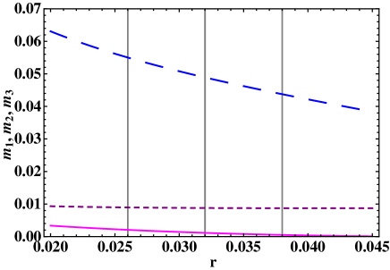
Figure 1: The light neutrino masses $m_{1}$ (solid line), $m_{2}$ (dashed line) and $m_{3}$ (long-dashed line) as functions of the parameter $r$ for $\Delta m^{2}_{21}=7.58\times 10^{-5}\leavevmode\nobreak\ {\rm eV^{2}}$. The three vertical lines correspond, from left to right, to $r=0.026,0.032,0.038$, i.e., to the $3\sigma$ minimal, best fit and $3\sigma$ maximal values of $r$. For $r=0.032$ we have: $m_{1}=1.14\times 10^{-3}$ eV, $m_{2}=8.788\times 10^{-3}$ eV, $m_{3}=4.89\times 10^{-2}$ eV.

IV The LFV Decays $\ell_{i}\rightarrow\ell_{j}+\gamma$

IV.1 The Decays $\ell_{i}\rightarrow\ell_{j}+\gamma$ in SUSY theories

In the minimal extended Standard Theory with heavy Majorana right-handed neutrinos, the simultaneous presence of neutrino and lepton Yukawa couplings, $Y_{\nu}$ and $Y_{e}$, leads to lepton flavour violation. In this scenario, the LFV decay rates and cross sections are strongly suppressed by the ratio Petcov:1976ff ; Bilenky:1977du $|(\sum_{j=2,3}U^{*}_{\mu j}U_{ej}\Delta m^{2}_{j1})/M^{2}_{W}|^{2}$, $M_{W}\cong 80$ GeV being the $W^{\pm}$-boson mass, leading to, e.g., BR($\mu\rightarrow e\gamma$)$<10^{-47}$. This renders the LFV decays and reactions unobservable in the ongoing and future planned experiments. The situation is the same in the non-SUSY type I see-saw models in which the heavy Majorana neutrino masses $M_{k}$ are only by few to several orders of magnitude smaller than the GUT scale $M_{X}\approx 2\times 10^{16}$ GeV Cheng:1980tp ; footn4 .

The present experimental upper bounds on the rates of the LFV decays $\ell_{i}\rightarrow\ell_{j}+\gamma$, $m_{\ell_{i}}>m_{\ell_{j}}$, $\ell_{1}\equiv e$, $\ell_{2}\equiv\mu$, $\ell_{3}\equiv\tau$, are given by MEG11 ; Nakamura:2010zzi

$$BR(\mu\rightarrow e\gamma)<2.4\times 10^{-12},\quad BR(\mu\rightarrow 3e)<1\times 10^{-12},\quad BR(\tau\rightarrow\mu\gamma)<4.4\times 10^{-8}.$$ (63)

The first was obtained recently in the MEG experiment at PSI and is an improvement by a factor of 5 of the previous best upper limit of the MEGA experiment, published in 1999 Brooks:1999pu . The projected sensitivity of the MEG experiment is MEG11 :

$$BR(\mu\rightarrow e\gamma)\sim 10^{-13}.$$ (64)

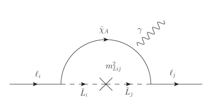
Figure 2: Feynman diagrams of the dominant contribution to the $\ell_{i}\rightarrow\ell_{j}+\gamma$ radiative decay amplitude in the mass insertion approximation. $\tilde{\chi}_{A}$ corresponds to charginos or neutralinos and $\tilde{L}_{i}$ are the slepton doublets. The photon can be emitted from the chargino or the slepton lines.

In the supersymmetric (SUSY) theories these decay rates can be largely enhanced due to contributions from the slepton part of the soft SUSY breaking Lagrangian, $\mathcal{L}_{soft}$:

$$-\mathcal{L}_{soft} = (m^{2}_{\tilde{L}})_{ij}\tilde{L}^{\dagger}_{i}\tilde{L}_{j}+(m^{2}_{\tilde{e}})_{ij}\tilde{e}^{\ast}_{Ri}\tilde{e}_{Rj}+(m^{2}_{\tilde{\nu}})_{ij}\tilde{\nu}^{\ast}_{Ri}\tilde{\nu}_{Rj}$$ (65)

$$+\left((A_{e})_{ij}H_{d}\tilde{e}^{\ast}_{Ri}\tilde{L}_{j}+(A_{\nu})_{ij}H_{u}\tilde{\nu}^{\ast}_{Ri}\tilde{L}_{j}+h.c.\right),$$

where $m^{2}_{\tilde{L}}$ and $m^{2}_{\tilde{e}}$ are the left-handed (LH) and right-handed (RH) charged slepton mass matrices, respectively, $m^{2}_{\tilde{\nu}}$ is the right-handed sneutrino soft mass term, $A_{e}$ and $A_{\nu}$ are trilinear couplings and $H_{d}$ and $H_{u}$ are the two Higgs doublet fields present in the SUSY theories. Non-zero off-diagonal elements in the slepton mass matrix could induce lepton flavour violation, but only relatively small values could satisfy the upper bounds quoted above. Soft-breaking terms are, however, subjected to renormalization through Yukawa and gauge interactions in such a way that LFV is induced in the slepton mass matrix at “low energies”. Indeed, in addition to a LF conserving part, the renormalisation group (RG) equation for the left handed slepton mass matrix present, in general, off-diagonal terms which are a source of LFV.

The indicated generic possibility is realized in the SUSY (GUT) theories with see-saw mechanism of neutrino mass generation BorzMas86 . If the SUSY breaking occurs via soft terms with universal boundary conditions at a scale $M_{X}$ above the RH Majorana neutrino mass scale $M_{R}$, $M_{X}>M_{R}$, as in the so-called minimal supergravity (mSUGRA) scenario Chamseddine:1982jx , the renormalisation group effects transmit the LFV from the neutrino mixing at $M_{X}$ to the effective mass terms of the scalar leptons at $M_{R}$, generating new LFV corrections to the flavour-diagonal mass terms. For slepton masses of a few hundred GeV, the LFV mass corrections at $M_{R}$ are typically of the order of a few GeV and thus are much larger than the light neutrino masses $m_{j}$ . As a consequence (and in contrast to the non-supersymmetric case), the LFV scalar lepton mixing at $M_{R}$ generates additional contributions to the amplitudes of the LFV decays and reactions which are not suppressed by the small values of neutrino masses. As a result, the LFV processes can proceed with rates and cross sections which are within the sensitivity of presently operating and future planned experiments BorzMas86 ; Hisano96 (see also, e.g., Casas:2001sr ; Ellis:2002eh ; Petcov:2003zb ; PS06 ; Raidal:2008jk and the references quoted therein).

In the following discussion we will assume the commonly employed mSUGRA SUSY breaking scenario Chamseddine:1982jx . In this scenario the flavour is assumed to be exactly conserved at the GUT scale, $M_{X}\approx 2\times 10^{16}$ GeV, by the soft SUSY breaking terms. More specifically, it is assumed that at the scale $M_{X}$ the slepton mass matrices are diagonal in flavour and universal, the trilinear couplings are proportional to the neutrino and charged lepton Yukawa couplings $Y_{\nu}$ and $Y_{e}$, respectively, and the gaugino masses have a common value:

$$(m^{2}_{\tilde{L}})_{ij} = (m^{2}_{\tilde{e}})_{ij}=(m^{2}_{\tilde{\nu}})_{ij}=\delta_{ij}m_{0}^{2}$$

$$A_{\nu} = Y_{\nu}a_{0}m_{0},\quad A_{e}=Y_{e}a_{0}m_{0}$$

$$M_{\tilde{B}} = M_{\tilde{W}}=M_{\tilde{g}}=m_{1/2}.$$ (66)

Hence the parameter space of interest of mSUGRA is determined by:

$$m_{1/2},\leavevmode\nobreak\ m_{0},\leavevmode\nobreak\ A_{0},\leavevmode\nobreak\ tg\beta\,,$$ (67)

$tg\beta$ being the ration of the vacuum expectation values of the Higgs fields $H_{u}$ and $H_{d}$.

In the leading-log approximation, the branching ratios of the LFV processes $\ell_{i}\rightarrow\ell_{j}+\gamma$ ($m_{l_{i}}>m_{l_{j}}$ ) is given by Hisano96 (see also, e.g., Casas:2001sr ; Ellis:2002eh ; Petcov:2003zb ; Raidal:2008jk ):

$$B(\ell_{i}\rightarrow\ell_{j}+\gamma)\cong\frac{\Gamma(\ell_{i}\rightarrow\ell_{j}\nu\bar{\nu})}{\Gamma_{tot}(\ell_{i})}B_{0}(m_{0},m_{1/2})\left|\sum_{k}(Y_{\nu})_{ik}\ln\frac{M_{X}}{M_{k}}\ln\frac{M_{X}}{M_{k}}(Y^{\dagger}_{\nu})_{kj}\right|^{2}\tan^{2}\beta.$$ (68)

Here $G_{F}$ is the Fermi constant, $\alpha_{em}\approx 1/137$ is the fine structure constant, $M_{k}$ is the mass of the heavy Majorana neutrino $N_{k}$, $Y_{\nu}$ is the matrix of neutrino Yukawa couplings in the basis in which the Majorana mass matrix of the RH neutrinos and the matrix of charged lepton Yukawa couplings are diagonal, and Nakamura:2010zzi $\Gamma(\mu\rightarrow e\nu\bar{\nu})/\Gamma_{tot}(\mu)\approx 1$, $\Gamma(\tau\rightarrow e\nu\bar{\nu})/\Gamma_{tot}(\tau)\approx 0.1785$, $\Gamma(\tau\rightarrow\mu\nu\bar{\nu})/\Gamma_{tot}(\tau)\approx 0.1736$. The scaling function $B_{0}(m_{0},m_{1/2})$ contains the dependence on the SUSY breaking parameters:

$$B_{0}(m_{0},m_{1/2})=\frac{\alpha_{em}^{3}}{G_{F}^{2}m_{S}^{8}}\left|\frac{(3+a_{0}^{2})m_{0}^{2}}{8\pi^{2}}\right|^{2}\,.$$ (69)

The effective SUSY mass parameter $m_{S}$ that appears in equation (68) can be approximated by Petcov:2003zb :

$$m_{S}^{8}\approx 0.5m^{2}_{0}m^{2}_{1/2}(m^{2}_{0}+0.6m^{2}_{1/2})^{2}$$ (70)

This analytic expression was shown to reproduce the exact RG results for $B(\ell_{i}\rightarrow\ell_{j}+\gamma)$ with high precision. In Fig. 3 we illustrate the dependence of the scaling function $B_{0}(m_{0},m_{1/2})$ on the parameter $m_{0}$ ($m_{1/2}$) for four values of $m_{1/2}$ ($m_{0}$).

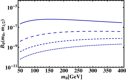
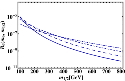
Figure 3: The scaling factor $B_{0}(m_{0},m_{1/2})$ as function of $m_{0}$ (left panel) and $m_{1/2}$ (right panel) for $A_{0}=7m_{0}$. Left panel: the values of $m_{1/2}$ used are 200 GeV (solid line), 400 GeV (long-dashed line), 600 GeV (medium long-dashed line), 800 GeV (short-dashed line). Right panel: the values of $m_{0}$ used are 50 GeV (solid line), 100 GeV (long-dashed line), 200 GeV (medium long-dashed line), 400 GeV (short-dashed line).

IV.2 Predictions of the $SU(5)\times T^{\prime}$ Model

As we have seen, in the $SU(5)\times T^{\prime}$ model of flavour we are considering the three heavy Majorana neutrinos $N_{j}$ are, to leading order, degenerate in mass: $M_{j}=s_{0}\Lambda\equiv M>0$, $j=1,2,3$. The higher order corrections to the masses $M_{j}$ lead to exceedingly small effects in the $\ell_{i}\rightarrow\ell_{j}+\gamma$ decay rates and we will neglect them. In this case the branching ratios $B(\ell_{i}\rightarrow\ell_{j}+\gamma)$ of interest, as it follows from eq. (68), depend on the quantity $|(Y_{\nu}Y^{\dagger}_{\nu})_{ij}|^{2}$.

As can be shown, in the model under study, the matrix of neutrino Yukawa couplings $Y_{\nu}$ entering into the expressions for $B(\ell_{i}\rightarrow\ell_{j}+\gamma)$ is related to the Dirac neutrino mass matrix $M_{D}$, eq. (24), as follows:

$$Y_{\nu}=\frac{1}{v_{u}}\,U^{\dagger}_{e}\,M_{D}\,S\,$$ (71)

where $U_{e}$ is the matrix diagonalising $M_{e}M^{\dagger}_{e}$, $M_{e}$ being the charged lepton mass matrix, and $S$ is determined in eqs. (27) and (28). In the basis in which the RH neutrino Majorana mass matrix and the matrix of charged lepton Yukawa couplings are diagonal, the Majorana mass term for the LH flavour neutrinos, generated by the see-saw mechanism, is given by:

$$M_{\nu}=-\,v^{2}_{u}\,Y_{\nu}D_{N}^{-1}Y_{\nu}^{T}=U^{\prime}\,D_{\nu}\,(U^{\prime})^{T}\;,\leavevmode\nobreak\$$ (72)

where $D_{\nu}\equiv diag(m_{1},m_{2},m_{3})$ and

$$U^{\prime}=U^{\dagger}_{e}U_{TBM}Q\,.$$ (73)

Equation (72), as is well known, allows to express $Y_{\nu}$ in terms of $U^{\prime}$, $D_{\nu}$, $D_{N}$ and a complex, in general, orthogonal matrix Casas:2001sr $R$, $R^{T}R=RR^{T}={\bf 1}$:

$$Y_{\nu}=\frac{1}{v_{u}}\,U^{\prime}\,\sqrt{D_{\nu}}\,R\,\sqrt{D_{N}}\,.$$ (74)

From eqs. (71) - (74) and (26), we obtain the following expression for the matrix $R$:

$$R=v_{u}\,(\sqrt{D_{\nu}})^{-1}\,Q^{*}\,\,M^{diag}_{D}\,\,U^{T}_{TBM}\ S\,(\sqrt{D_{N}})^{-1}\,.$$ (75)

Using the explicit form of $Q=diag(1,1,\pm i)$ and of $U_{TBM}$ and $S$, eqs. (6) and (28), it is not difficult to show that $R$ is a real matrix: $R^{*}=R$. Taking into account this result and recalling that $D_{N}=M\,diag(1,1,1)$, we get for the quantity of interest $Y_{\nu}Y^{\dagger}_{\nu}$:

$$Y_{\nu}Y^{\dagger}_{\nu}=\frac{M}{v^{2}_{u}}\,U^{\prime}\,D_{\nu}\,(U^{\prime})^{\dagger}\,,$$ (76)

where the PMNS matrix $U^{\prime}=U^{\dagger}_{e}U_{TBM}Q$, see eqs. (49), (41), (49) and (54). Thus, the $\ell_{i}\rightarrow\ell_{j}+\gamma$ decay branching ratios in the $SU(5)\times T^{\prime}$ model under investigation depend on the mass of the heavy Majorana neutrinos through the factor $(M(\ln M_{X}/M_{k})/v_{u})^{2}$, do not depend on the matrix $R$, and their ratios are entirely determined by the elements of the PMNS matrix and the light neutrino masses. More specifically, using the general expressions for the elements of the PMNS matrix and the unitarity of the latter we get PS06 :

$$\left|(Y_{\nu}Y^{\dagger}_{\nu})_{\mu e}\right|=\left|U_{\mu j}m_{j}U^{*}_{ej}\right|\simeq\left|\Delta_{21}\,s_{12}c_{23}c_{12}+\Delta_{31}\,s_{23}s_{13}e^{i\delta}\right|\,,$$ (77)

$$\left|(Y_{\nu}\,Y^{\dagger}_{\nu})_{\tau e}\right|=\left|U_{\tau j}\,m_{j}\,U^{*}_{ej}\right|\simeq\left|-\,\Delta_{21}\,s_{12}c_{12}s_{23}+\Delta_{31}\,c_{23}s_{13}e^{i\delta}\right|\,,$$ (78)

$$\left|(Y_{\nu}\,Y^{\dagger}_{\nu})_{\tau\mu}\right|=\left|U_{\tau j}\,m_{j}\,U^{*}_{\mu j}\right|\simeq\left|\Delta_{31}\,c_{23}s_{23}\right|\,,$$ (79)

where

$$\Delta_{ij}=\frac{M_{R}}{v_{u}^{2}}\frac{\Delta m^{2}_{ij}}{m_{i}+m_{j}}\,.$$ (80)

In eqs. (77) - (79) we have used the approximation $c_{13}\cong 1$ and have neglected $c^{2}_{12}\Delta_{21}$, $s^{2}_{12}\Delta_{21}$ and higher order terms $\propto\Delta_{21}$ with respect to $\Delta_{31}$.

We define the “double” ratios of the branching ratios $B(\ell_{i}\rightarrow\ell_{j}+\gamma)$ as follows:

$$R(21/31)\equiv\frac{BR(\mu\rightarrow e\gamma)}{BR(\tau\rightarrow e\gamma)}BR(\tau\rightarrow e\nu_{\tau}\bar{\nu}_{e}),\quad R(21/32)\equiv\frac{BR(\mu\rightarrow e\gamma)}{BR(\tau\rightarrow\mu\gamma)}BR(\tau\rightarrow e\nu_{\tau}\bar{\nu}_{e})$$ (81)

The double ratios of interest are given by:

$$R(21/31)\cong\frac{|(Y_{\nu}Y^{\dagger}_{\nu})_{\mu e}|^{2}}{|(Y_{\nu}Y^{\dagger}_{\nu})_{\tau e}|^{2}}\,,\\ \quad R(21/32)\cong\frac{|(Y_{\nu}Y^{\dagger}_{\nu})_{\mu e}|^{2}}{|(Y_{\nu}Y^{\dagger}_{\nu})_{\tau\mu}|^{2}}\,.$$ (82)

IV.3 Numerical Results

In Figs. 4 - 7 we present results on the branching ratios $BR(\mu\rightarrow e+\gamma)$, $BR(\tau\rightarrow e+\gamma)$ and $BR(\tau\rightarrow\mu+\gamma)$, predicted by the $SU(5)\times T^{\prime}$ model. The branching ratios are calculated using eq. (68) with $M_{k}$ and $M_{X}$ set to $M_{k}=M=10^{12}$ GeV and $M_{X}=2\times 10^{16}$ GeV. The values of the mSUGRA parameters $\tan\beta$ and $A_{0}$ are chosen from the intervals $\tan\beta=3\div 50$, $A_{0}=0\div 7m_{0}$, which are compatible with the constaints obtained by the ATLAS Aad:2011hh ; Zhuang:2011qq and CMS Khachatryan:2011tk experiments at LHC. The values of the other two relevant mSUGRA parameters, $m_{0}$ and $m_{1/2}$, are chosen from intervals favored by the global data analysis performed Buchmueller:2011aa . The data set used in this analysis includes in addition to the results of the ATLAS and the CMS experiments, the data on the muon $(g-2)$, on the precision electroweak observables, on $B$-physics observables, astrophysical data on the cold dark matter density, as well as the limits from the direct searches for Higgs boson and sparticles at LEP. Based on the results obtained in Buchmueller:2011aa , $m_{0}$ and $m_{1/2}$ are chosen from, or to vary in, the intervals $50\leavevmode\nobreak\ {\rm GeV}\leq m_{0}\leq 400$ GeV and $300\leavevmode\nobreak\ {\rm GeV}\leq m_{1/2}\leq 800$ GeV. For the values of the lepton mixing angles and the Dirac phase $\delta$ we use those predicted (to leading order) by the $SU(5)\times T^{\prime}$ model (unless otherwise stated): $\sin^{2}\theta_{23}=0.5$, $\sin^{2}\theta_{12}=0.299$, $\sin\theta_{13}=0.058$, $\delta=5\pi/4$. The neutrino masses used as input are obtained using the best fit values of $\Delta m^{2}_{21}=7.58\times 10^{-5}\leavevmode\nobreak\ {\rm eV^{2}}$ and $r=0.032$.

Figure 4: The branching ratios BR($\mu\rightarrow e+\gamma$) (left), BR($\tau\rightarrow e+\gamma$) (center) and BR($\tau\rightarrow\mu+\gamma$) (right) as function of $m_{0}$ for $\Delta m^{2}_{21}=7.58\times 10^{-5}\leavevmode\nobreak\ {\rm eV^{2}}$, $r=0.032$, $\delta=5\pi/4$, $\sin\theta_{13}$= 0.058, $\tan\beta=28$, $A_{0}$= 7$m_{0}$, and three values of $m_{1/2}$: 400 GeV (solid line), 600 GeV (dashed line), 800 GeV (dotted line). The horizontal line corresponds to the MEG bound BR($\mu\rightarrow e+\gamma$)$<2.4\times 10^{-12}$. See text for details.

Figure 5: The branching ratios $BR(\mu\rightarrow e+\gamma)$ (left), $BR(\tau\rightarrow e+\gamma)$ (center) and $BR(\tau\rightarrow\mu+\gamma)$ (right) as function of $m_{1/2}$ for three values of $m_{0}$: 50 GeV (solid line), 150 GeV (dashed line), 250 GeV (dotted line). The values of the other parameters used are the same as those quoted in the caption of Fig. 4. The horizontal line corresponds to the MEG bound BR($\mu\rightarrow e+\gamma$)$<2.4\times 10^{-12}$.

As the Figs. 4 - 7 show, for the values of $M=10^{12}$ GeV and $\tan\beta=28$ considered and $m_{0}$ from the interval (50 - 400) GeV, the predictions for the branching ratios $BR(\mu\rightarrow e\gamma)$, $BR(\tau\rightarrow e\gamma)$ and $BR(\tau\rightarrow\mu\gamma)$ are very sensitive to the values of $m_{1/2}$: when the latter increases from 300 GeV to 800 GeV, the branching ratios decrease by approximately 2 orders of magnitude. For the fixed value of $A_{0}=430$ GeV, we have $BR(\mu\rightarrow e\gamma)\ \raisebox{-1.72218pt}{\hbox to0.0pt{$\sim$\hss}}\raisebox{1.72218pt}{$>$}\ 10^{-13}$ provided

Figure 6: The branching ratios BR($\mu\rightarrow e+\gamma$) (left), BR($\tau\rightarrow e+\gamma$) (center) and BR($\tau\rightarrow\mu+\gamma$) (right) as function of $m_{0}$ for $A_{0}=430$ GeV and three values of $m_{1/2}$: 400 GeV (solid line), 600 GeV (dashed line), 800 GeV (dotted line). The values of the other parameters used are the same as those quoted in the caption of Fig. 4. The horizontal line corresponds to the MEG bound $BR(\mu\rightarrow e+\gamma)<2.4\times 10^{-12}$.

Figure 7: The branching ratios BR($\mu\rightarrow e+\gamma$) (left), BR($\tau\rightarrow e+\gamma$) (center) and BR($\tau\rightarrow\mu+\gamma$) (right) as function of $m_{1/2}$ for $A_{0}=430$ GeV and $m_{0}=150$ GeV (solid line), 250 GeV (dashed line). The values of the other parameters used are the same as those quoted in the caption of Fig. 4. The horizontal dashed line corresponds to the MEG bound BR($\mu\rightarrow e+\gamma)<2.4\times 10^{-12}$.

$m_{0}\ \raisebox{-1.72218pt}{\hbox to0.0pt{$\sim$\hss}}\raisebox{1.72218pt}{$<$}\ 300$ GeV and $m_{1/2}\ \raisebox{-1.72218pt}{\hbox to0.0pt{$\sim$\hss}}\raisebox{1.72218pt}{$<$}\ 400$ GeV (Figs. 6 and 7). The ranges of values of $m_{0}$ and $m_{1/2}$, for which $10^{-13}\ \raisebox{-1.72218pt}{\hbox to0.0pt{$\sim$\hss}}\raisebox{1.72218pt}{$<$}\ BR(\mu\rightarrow e\gamma)<2.4\times 10^{-12}$, is very different in the case when $A_{0}\propto m_{0}$. For $A_{0}=7m_{0}$ ( Figs. 4 - 5), for instance, $BR(\mu\rightarrow e\gamma)$ satisfies the MEG upper limit and is in

Figure 8: The branching ratio BR($\mu\rightarrow e+\gamma$) as function of $\theta_{13}$ (left panel) and of the Dirac phase $\delta$ (right panel) for $r=0.032$, $m_{0}=230$ GeV, $m_{1/2}=400$ GeV, $A_{0}=430$ GeV and $\tan\beta=28$. In the left panel, $BR(\mu\rightarrow e+\gamma)$ is plotted for three values of $\delta$: $\pi/2$ (solid line) , $\pi$ (dashed line), $5\pi/4$ (dotted line). The horizontal line corresponds to the MEG bound $BR(\mu\rightarrow e+\gamma)<2.4\times 10^{-12}$. The results for $BR(\mu\rightarrow e+\gamma)$ shown in the right panel are obtained for $\sin\theta_{13}=0.058$. The solid vertical line in the right panel corresponding to $\delta=5\pi/4$.

the range of sensitivity of the MEG experiment for $m_{0}$ lying in the interval $m_{0}\cong(100-300)$ GeV if $600\leavevmode\nobreak\ {\rm GeV}\ \raisebox{-1.72218pt}{\hbox to0.0pt{$\sim$\hss}}\raisebox{1.72218pt}{$<$}\ m_{1/2}\ \raisebox{-1.72218pt}{\hbox to0.0pt{$\sim$\hss}}\raisebox{1.72218pt}{$<$}\ 800$ GeV. For the values of the parameters used to obtain Figs. 4 - 7, we find that $BR(\tau\rightarrow\mu+\gamma)\ \raisebox{-1.72218pt}{\hbox to0.0pt{$\sim$\hss}}\raisebox{1.72218pt}{$<$}\ 10^{-9}$ and $BR(\tau\rightarrow e+\gamma)\ \raisebox{-1.72218pt}{\hbox to0.0pt{$\sim$\hss}}\raisebox{1.72218pt}{$<$}\ 3\times 10^{-11}$.

The $\mu\rightarrow e+\gamma$ decay branching ratio $BR(\mu\rightarrow e+\gamma)$ can exhibit very strong dependence on the value of the angle $\theta_{13}$ if the Dirac phase $\delta\cong\pi$, and on the Dirac phase $\delta$ in the case of $\sin\theta_{13}=0.058$. This is illustrated in Fig. 8 and can be easily understood on the basis of the analytic expression for $|(Y_{\nu}Y^{\dagger}_{\nu})_{\mu e}|$ given in eq. (77). As Fig. 8 shows, for the values of $\delta=5\pi/4$ and $\sin\theta_{13}=0.058$, predicted by the model, $BR(\mu\rightarrow e\gamma)$ is somewhat smaller than the maximal value it can have as a function of $\delta$ and $\sin\theta_{13}$.

We have studied also the dependence of the $\mu\rightarrow e+\gamma$ decay branching ratio $BR(\mu\rightarrow e+\gamma)$ on the parameter $r$. The results of this study are illustrated in Fig. 9 for three values of $\sin^{2}\theta_{13}$, $\sin^{2}\theta_{13}=3.4\times 10^{-3},0.01,0.02$, and three values of $\delta$, $\delta=\pi/2,\pi,5\pi/4$. For illustrative purposes the ratio $r$ is varied in the interval $0\leq r\leq 0.05$, which is wider than the current $3\sigma$ range of allowed values of $r$, $0.026\leq r\leq 0.038$. Figure 9 exhibits in a different way the sensitivity of $BR(\mu\rightarrow e+\gamma)$ to the values of $\theta_{13}$ and $\delta$.

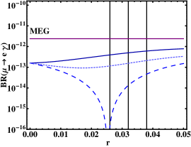
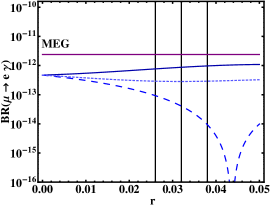
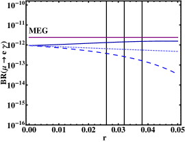
Figure 9: The dependence of the branching ratio BR($\mu\rightarrow e+\gamma$) on the parameter $r$ for $m_{0}=230$ GeV, $m_{1/2}=400$ GeV, $A_{0}=430$ GeV and $\tan\beta=28$. The left, middle and right panels are obtained for $\sin^{2}\theta_{13}=3.4\times 10^{-3}$ Chen:2009gf , 0.01 and 0.02, respectively. The values of $\delta$ used are $\pi/2$ (solid line), $\pi$ (dashed line) and $5\pi/4$ (dotted line). The vertical lines correspond respectively to $r=$0.026, 0.032, 0.038. The horizontal line shows the MEG bound $BR(\mu\rightarrow e+\gamma)<2.4\times 10^{-12}$. See text for details.

In Fig. 10 we present results the double ratios $R(21/31)$ and $R(21/32)$ predicted by the model, as a function of the lightest neutrino mass $m_{1}$. We recall that the double ratios $R(21/31)$ and $R(21/32)$ in the model considered do not depend on the heavy Majorana neutrino mass $M$ and on the mSUGRA parameters: they are entirely determined by the values of the neutrino masses, the neutrino mixing angles and the Dirac CP violating phase $\delta$. All these neutrino parameters have essentially definite values in the $SU(5)\times T^{\prime}$ model considered. Thus, the values of the double ratios $R(21/31)$ and $R(21/32)$ are predicted by the model with relatively small uncertainties, as is also seen in Fig. 10: we have numerically

$$R(21/31)\cong 0.21,\leavevmode\nobreak\ \leavevmode\nobreak\ \leavevmode\nobreak\ R(21/32)\cong 7.4\times 10^{-3}\,.$$ (83)

These values are one of the characteristic predictions of the $SU(5)\times T^{\prime}$ model of flavour under investigation. It is interesting to note also that in the model with $SU(5)\times T^{\prime}$ symmetry considered, the $\tau\rightarrow\mu+\gamma$ decay branching ratio $BR(\tau\rightarrow\mu+\gamma)/BR(\tau\rightarrow e\nu_{\tau}\bar{\nu}_{e})$ can be bigger than the $\mu\rightarrow e+\gamma$ decay branching ratio $BR(\mu\rightarrow e+\gamma)$ by a factor $\sim 10^{2}$.

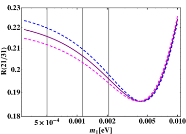
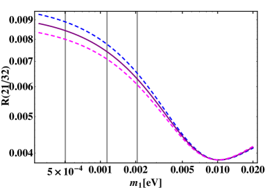
Figure 10: The double ratios R(21/31), left panel, and R(21/32), right panel, as functions of the lightest neutrino mass, $m_{1}$. The three vertical lines in each plot are positioned at $m_{1}=2.06\times 10^{-3},1.14\times 10^{-3},\leavevmode\nobreak\ 5.0\times 10^{-4}$ eV, and correspond to $r=0.026,0.032,0.038$ and the best fist value of $\Delta m^{2}_{21}=7.58\times 10^{-5}\leavevmode\nobreak\ {\rm eV^{2}}$. The solid lines are obtained with the best-fit values of $\Delta m^{2}_{21}$ and $\Delta m^{2}_{31}$ given in Table 1, while the dashed lines indicate the $3\sigma$ allowed ranges.

V Conclusions

In the present article we have investigate certain aspects of the low energy lepton phenomenology of the SUSY $SU(5)\times T^{\prime}$ model of flavour which was developed in  Chen:2007afa ; Chen:2009gf , and which allows to describe in a unified way the masses and the mixing of the quarks and the leptons, neutrinos included, as well as the CP violation both in the quark and lepton sectors. The model includes three right-handed neutrino fields which possess a Majorana mass term. The light neutrino masses are generated by the type I see-saw mechanism and are naturally small. The light and heavy neutrinos are Majorana particles. The heavy Majorana neutrinos $N_{k}$ are predicted (to leading order) to be degenerate in mass: $M_{k}=M$. The model is free of discrete gauge anomalies. In addition to giving rise to realistic masses and mixing patterns for the leptons and quarks, a unique feature of the $SU(5)\times T^{\prime}$ model is that the CP violation, predicted by the model, is entirely geometrical in origin. This interesting aspect of the model considered is a consequence of the special properties of the group $T^{\prime}$. The model was shown to predict approximately tri-bimaximal neutrino (TBM) mixing with deviations which generate a non-zero $\sin\theta_{13}=\sin\theta_{c}/(3\sqrt{2})$, where $\theta_{c}$ is the Cabibbo angle, and a Dirac phase $\delta=221^{\circ}\cong 5\pi/4$. A rather detailed description of the lepton sector of the model is given in Section 2.

We have derived first the predictions of the model for the light Majorana neutrino masses, $m_{i}$, $i=1,2,3$. We have found that in the model considered only light neutrino mass spectrum with normal ordering (or normal hierarchy) is possible. In the standardly used convention this implies $m_{1}<m_{2}<m_{3}$. The masses $m_{i}$ depend on two parameters of the model which, as we have shown, can be fixed using the values of $\Delta m^{2}_{21}$, which drives the solar neutrino oscillations, and the ratio $r=\Delta m^{2}_{21}/\Delta m^{2}_{31}$, $\Delta m^{2}_{31}$ being the neutrino mass squared difference responsible for the dominant atmospheric $\nu_{\mu}$ and $\bar{\nu}_{\mu}$ oscillations. Given the fact that $\Delta m^{2}_{21}$ and $r$ have been determined experimentally with rather small uncertainties, the light neutrino masses are predicted to lie in relatively narrow intervals around the values $m_{1}=1.14\times 10^{-3}$ eV, $m_{2}=8.78\times 10^{-3}$ eV, $m_{3}=4.89\times 10^{-2}$ eV (Fig. 1). As a consequence, the model provides specific predictions for the sum of the light neutrino masses in terms of $\Delta m^{2}_{21}$ and $r$: $m_{1}+m_{2}+m_{3}\cong\Delta m^{2}_{21}(1+(20r-1)^{2}+(20r-3)^{2})(1-(20r-1)^{4})^{-\frac{1}{2}}$. Numerically, we have found: $m_{1}+m_{2}+m_{3}\cong 5.9\times 10^{-2}\leavevmode\nobreak\ {\rm eV}$.

The model provides also specific prediction for the effective Majorana mass in neutrinoless double beta ($(\beta\beta)_{0\nu}$-decay), $\left|<\!m\!>\right|\$. The two Majorana phases $\alpha_{21}$ and $\alpha_{31}$ in the neutrino mixing matrix (see eqs. (1 - (3)) are predicted (to leading order) to have CP conserving values: $\alpha_{21}=0$ and $\alpha_{31}=\pi$. We found that the effective Majorana mass predicted by the model is given approximately by: $\mbox{$\left|<\!m\!>\right|\ $}\cong|(2m_{1}+m_{2})/3-\sqrt{2}(m_{2}-m_{1})(\sin\theta_{c})/9|$. Numerically, we obtained $\mbox{$\left|<\!m\!>\right|\ $}\cong 3.4\times 10^{-3}$ eV.

In the last part of this work we have derived detailed predictions for the rates of the lepton flavour violating (LFV) charged lepton radiative decays $\mu\rightarrow e+\gamma$, $\tau\rightarrow e+\gamma$ and $\tau\rightarrow\mu+\gamma$. This was done within the commonly employed mSUGRA SUSY breaking scenario Chamseddine:1982jx . The values of the mSUGRA parameters $\tan\beta$ and $A_{0}$ are chosen from the intervals $\tan\beta=3\div 50$, $A_{0}=0\div 7m_{0}$, which are compatible with the constraints obtained by the ATLAS Aad:2011hh ; Zhuang:2011qq and CMS Khachatryan:2011tk experiments at LHC. The values of the other two relevant mSUGRA parameters, $m_{0}$ and $m_{1/2}$, are chosen from intervals favored by the global data analysis performed in Buchmueller:2011aa . The data set used in this analysis includes in addition to the results of the ATLAS and the CMS experiments, the data on the muon $(g-2)$, on the precision electroweak observables, on $B$-physics observables, astrophysical data on the cold dark matter density, as well as the limits from the direct searches for Higgs boson and sparticles at LEP. Based on the results obtained in Buchmueller:2011aa , $m_{0}$ and $m_{1/2}$ are chosen from, or to vary in, the intervals $50\leavevmode\nobreak\ {\rm GeV}\leq m_{0}\leq 400$ GeV and $300\leavevmode\nobreak\ {\rm GeV}\leq m_{1/2}\leq 800)$ GeV. The branching ratios are calculated for masses of the heavy Majorana neutrinos $M_{k}=M=10^{12}$ GeV. The GUT scale used is $M_{X}=2\times 10^{16}$ GeV. The results of the this analysis are reported graphically in Figs. 4 - 10.

One specific prediction of the $SU(5)\times T^{\prime}$ model of flavour considered is that the quantity $|(Y_{\nu}Y^{\dagger}_{\nu})_{ll^{\prime}}|$ on which the $l\rightarrow l^{\prime}+\gamma$ decay branching ratios depend, $l=\mu,\tau$, $l^{\prime}=e,\mu$ ($m_{l}>m_{l^{\prime}}$), $Y_{\nu}$ being the matrix of neutrino Yukawa couplings in the basis in which the RH neutrino Majorana mass term and the matrix of charged lepton Yukawa couplings are diagonal, is a function of the PMNS neutrino mixing matrix $U$ and neutrino masses $m_{i}$ only, $|(Y_{\nu}Y^{\dagger}_{\nu})_{ll^{\prime}}|=|U_{lj}m_{j}U^{*}_{l^{\prime}j}|$. Thus, in the model considered and for given $l$ and $l^{\prime}$ this quantity is fixed numerically with small uncertainties. Together with the fact that the heavy Majorana neutrinos are degenerate in mass, this feature of the model implies that the double ratios of the branching ratios $R(21/31)\equiv(BR(\mu\rightarrow e+\gamma)/BR(\tau\rightarrow e+\gamma))BR(\tau\rightarrow e\nu_{\tau}\bar{\nu}_{e})$ and $R(21/32)\equiv(BR(\mu\rightarrow e+\gamma)/BR(\tau\rightarrow\mu+\gamma))BR(\tau\rightarrow e\nu_{\tau}\bar{\nu}_{e})$ do not depend not only on the mSUGRA parameters, but also on the heavy Majorana neutrino masses and the GUT scale $M_{X}$: $R(21/31)\cong|(Y_{\nu}Y^{\dagger}_{\nu})_{\mu e}|^{2}/|(Y_{\nu}Y^{\dagger}_{\nu})_{\tau e}|^{2}$, $R(21/32)\cong|(Y_{\nu}Y^{\dagger}_{\nu})_{\mu e}|^{2}/|(Y_{\nu}Y^{\dagger}_{\nu})_{\tau\mu}|^{2}$. Numerically we have found: $R(21/31)\cong 0.21$, $R(21/32)\cong 7.4\times 10^{-3}$. These values are one of the characteristic predictions of the model with $SU(5)\times T^{\prime}$ symmetry considered. In particular, the $\tau\rightarrow\mu+\gamma$ decay branching ratio, $BR(\tau\rightarrow\mu+\gamma)/BR(\tau\rightarrow e\nu_{\tau}\bar{\nu}_{e})$, is predicted to be bigger than the $\mu\rightarrow e+\gamma$ decay branching ratio, $BR(\mu\rightarrow e+\gamma)$, by a factor of $1.36\times 10^{2}$. We have found also that in a relatively large part of the mSUGRA parameter space considered and for $M=10^{12}$ GeV, the $\mu\rightarrow e\gamma$ decay branching ratio can satisfy the MEG upper bound $BR(\mu\rightarrow e+\gamma)<2.4\times 10^{-12}$, but still can have a value in the range of sensitivity of the MEG experiment, $BR(\mu\rightarrow e+\gamma)\ \raisebox{-1.72218pt}{\hbox to0.0pt{$\sim$\hss}}\raisebox{1.72218pt}{$>$}\ 10^{-13}$.

The model with $SU(5)\times T^{\prime}$ symmetry proposed in  Chen:2007afa ; Chen:2009gf and investigated in the present article provides a unified description of the masses and mixing of the quarks and leptons, neutrinos included, as well as of the CP violation both in the quark and lepton sectors. This makes it a viable model of flavour, which possesses a number of appealing features. In the lepton sector the model provides specific predictions for the values of the light neutrino masses, the neutrino mass spectrum, the values of the neutrino mixing angles, including the smallest one $\theta_{13}$, and the Dirac and Majorana CP violation phases in the neutrino mixing matrix. All these predictions can and will be tested in the currently operating and future neutrino experiments. We are looking forward to the outcome of these tests.

References

- (1) K. Nakamura and S.T. Petcov, “Neutrino Mass, Mixing, and Oscillations”, in K. Nakamura et al. (Particle Data Group), J. Phys. G 37, 075021 (2010).
- (2) S.M. Bilenky, J. Hosek and S.T. Petcov, Phys. Lett. B 94 (1980) 495.
- (3) K. Abe et al. [T2K Collaboration], Phy. Rev. Lett. 107 (2011) 041801.
- (4) P. Adamson et al. [MINOS Collaboration], arXiv:1108.1509.
- (5) G. L. Fogli, E. Lisi, A. Marrone, A. Palazzo, A. M. Rotunno, arXiv:1106.6028 (to be published in Phys. Rev. D).
- (6) This result can have important implications for the “flavoured” leptogenesis scenario of generation of the baryon asymmetry of the Universe EMSTP08 .
- (7) E. Molinaro and S.T. Petcov, Phys. Lett. B 671 (2009) 60.
- (8) See the plenary talk by Y. Takeuichi at Neutrino 2010.
- (9) T. Schwetz, M. Tortola and J.W.F. Valle, arXiv:1108.1376.
- (10) F. Ardellier et al. [Double Chooz Collaboration], hep-ex/0606025.
- (11) See, e.g. the Daya Bay homepage http://dayawane.ihep.ac.cn/.
- (12) J.K. Ahn et al. [RENO Collaboration], arXiv:1003.1391.
- (13) M. Mezzetto and T. Schwetz, J. Phys. G 37 (2010) 103001 [arXiv:1003.5800].
- (14) L. Wolfenstein, Phys. Rev. D 18, 958 (1978); P. F. Harrison, D. H. Perkins and W. G. Scott, Phys. Lett. B 530, 167 (2002), and Phys. Lett. B 535, 163 (2002).
- (15) P. H. Frampton, S. T. Petcov and W. Rodejohann, Nucl. Phys. B 687, 31 (2004).
- (16) M.-C. Chen and K. T. Mahanthappa, Phys. Lett. B 652, 34 (2007); arXiv:0710.2118.
- (17) M.-C. Chen and K. T. Mahanthappa, Phys. Lett. B 681, 444 (2009); PoS ICHEP2010, 407 (2010) [arXiv:1011.6364]; arXiv:1012.1595.
- (18) Z. Z. Xing, Phys. Lett. B 533, 85 (2002); A. Zee, Phys. Rev. D 68, 093002 (2003); N. Li and B. Q. Ma, Phys. Rev. D 71, 017302 (2005); F. Plentinger and W. Rodejohann, Phys. Lett. B 625, 264 (2005); S. F. King, JHEP 0508, 105 (2005); I. Masina, Phys. Lett. B 633, 134 (2006); S. Antusch and S. F. King, Phys. Lett. B 631, 42 (2005);
- (19) K.A. Hochmuth, S.T. Petcov and W. Rodejohann, Phys. Lett B 654 (2007) 177.
- (20) D. Marzocca, S. T. Petcov, A. Romanino and M. Spinrath, arXiv:1108.0614.
- (21) A. Romanino, Phys. Rev. D 70, 013003 (2004).
- (22) E. Ma and G. Rajasekaran, Phys. Rev. D 64, 113012 (2001); E. Ma, ibid. 70, 031901 (2004); K. S. Babu, E. Ma and J. W. F. Valle, Phys. Lett. B 552, 207 (2003); G. Altarelli and F. Feruglio, Nucl. Phys. B 720, 64 (2005).
- (23) E. Ma, Mod. Phys. Lett. A 17, 627 (2002); X. G. He, Y. Y. Keum and R. R. Volkas, JHEP 0604, 039 (2006); E. Ma, H. Sawanaka and M. Tanimoto, Phys. Lett. B 641, 301 (2006); S. F. King and M. Malinsky, Phys. Lett. B 645, 351 (2007); S. Morisi, M. Picariello and E. Torrente-Lujan, Phys. Rev. D 75, 075015 (2007).
- (24) P. H. Frampton and T. W. Kephart, Int. J. Mod. Phys. A 10, 4689 (1995); [arXiv:hep-ph/9409330]. A. Aranda, C. D. Carone and R. F. Lebed, Phys. Rev. D 62, 016009 (2000); F. Feruglio, C. Hagedorn, Y. Lin and L. Merlo, Nucl. Phys. B 775, 120 (2007); P. H. Frampton and S. Matsuzaki, arXiv:0902.1140.
- (25) C. Luhn, Phys. Lett. B 670, 390 (2009).
- (26) Anomaly cancellation conditions have been utilized to give constraints on charges under a family symmetry based on , see, e.g., M.-C. Chen, A. de Gouvea and B. A. Dobrescu, Phys. Rev. D 75, 055009 (2007); M.-C. Chen, D. R. T. Jones, A. Rajaraman and H. B. Yu, ibid. 78, 015019 (2008); M.-C. Chen and J. Huang, Phys. Rev. D 81, 055007 (2010); ibid. 82, 075006 (2010); arXiv:1011.0407.
- (27) J.-Q. Chen and P.-D. Fan, J. Math. Phys. 39, 5519 (1998).
- (28) M. C. Chen and K. T. Mahanthappa, arXiv:1107.3856.
- (29) M.-C. Chen and K. T. Mahanthappa, under preparation.
- (30) For general conditions to obtain form diagonalizable neutrino mass matrix, see M.-C. Chen and S. F. King, JHEP 0906, 072 (2009).
- (31) Similar relation has been found in other contexts. See also, J. Ferrandis and S. Pakvasa, Phys. Rev. D 71, 033004 (2005); S. Antusch and S. F. King, Phys. Lett. B 631, 42 (2005).
- (32) P. I. Krastev and S. T. Petcov, Phys. Lett. B 205, 84 (1988).
- (33) C. Jarlskog, Z. Phys. C 29 491 (1985); Phys. Rev. Lett. 55, 1039 (1985).
- (34) S. M. Bilenky and S. T. Petcov, Rev. Mod. Phys. 59 (1987) 671; S.M. Bilenky, S. Pascoli and S.T. Petcov, Phys. Rev. D64 (2001) 053010; S. Pascoli and S.T. Petcov, Phys. Rev. D 77 (2008) 113003.
- (35) S. T. Petcov, Sov. J. Nucl. Phys. 25 (1977) 340 [Yad. Fiz. 25 (1977 641]; (E), 25 (1977) 698 [(E)25 (1977) 1336].
- (36) S. M. Bilenky, S. T. Petcov and B. Pontecorvo, Phys. Lett. B 67 (1977) 309.
- (37) T. P. Cheng and L. F. Li, Phys. Rev. Lett. 45 (1980) 1908.
- (38) The situation can be very different in TeV scale type I see-saw non-SUSY models, in which the rates and cross sections of the LFV processes under discussion can be close to the existing upper limits, see, e.g., A. Ibarra, E. Molinaro and S.T. Petcov, Phys. Rev. D 84 (2011) 013005.
- (39) J. Adam et al. [MEG Collaboration], arXiv:1107.5547.
- (40) K. Nakamura et al. [Particle Data Group], J. Phys. G 37 (2010) 075021.
- (41) M. L. Brooks et al. [MEGA Collaboration], Phys. Rev. Lett. 83 (1999) 1521
- (42) F. Borzumati and A. Masiero, Phys. Rev. Lett. 57 (1986) 961.
-
(43)
A. H. Chamseddine, R. L. Arnowitt and P. Nath,
Phys. Rev. Lett. 49 (1982) 970.
R. Barbieri, S. Ferrara and C. A. Savoy, Phys. Lett. B 119 (1982) 343. L. J. Hall, J. D. Lykken and S. Weinberg, Phys. Rev. D 27 (1983) 2359. - (44) J. Hisano et al., Phys. Lett. B357 (1995) 579; Phys. Rev. D53 (1996) 2442; J. Hisano and D. Nomura, Phys. Rev. D59 (1999) 116005.
- (45) J. A. Casas and A. Ibarra, Nucl. Phys. B 618 (2001) 171.
- (46) J. R. Ellis, M. Raidal and T. Yanagida, Phys. Lett. B 546 (2002) 228; S. Pascoli, S. T. Petcov and W. Rodejohann, Phys. Rev. D 68 (2003) 093007; S. Lavignac, I. Masina and C. A. Savoy, Phys. Lett. B520 (2001) 269; S. Pascoli, S. T. Petcov and C. E. Yaguna, Phys. Lett. B 564 (2003) 241; I. Masina and C. A. Savoy, Phys. Rev. D 71 (2005) 093003; S.T. Petcov, T. Shindou and Y. Takanishi, Nucl. Phys. B 738 (2006) 219.
- (47) S. T. Petcov, S. Profumo, Y. Takanishi and C. E. Yaguna, Nucl. Phys. B 676 (2004) 453
- (48) S.T. Petcov and T. Shindou, Phys. Rev. D 74 (2006) 073006.
- (49) M. Raidal et al., Eur. Phys. J. C 57 (2008) 13 [arXiv:0801.1826].
- (50) G. Aad et al. [ATLAS Collaboration], Phy. Rev. Lett. 106 (2011) 131802
- (51) X. Zhuang [ATLAS Collaboration], arXiv:1104.2907.
- (52) V. Khachatryan et al. [CMS Collaboration], Phys. Lett. B 698 (2011) 196
- (53) O. Buchmueller et al., Eur. Phys. J. C 71 (2011) 1634