Feldman-Cousins Confidence Levels – Toy MC Method

Abstract

In particle physics, the likelihood ratio ordering principle is frequently used to determine confidence regions. This method has statistical properties that are superior to that of other confidence regions. But it often requires intensive computations involving thousands of toy Monte Carlo datasets. The original paper by Feldman and Cousins contains a recipe to perform the toy MC computation. In this note, we explain their recipe in a more algorithmic way, show its connection to $1-\rm CL$ plots, and apply it to simple Gaussian situations with boundaries.

I Likelihood ratio ordering

Feldman and Cousins have developed a method Feldman:1997qc to compute confidence intervals that has well-defined frequentist coverage. Their method has certain advantages over the classical approach to compute confidence levels: it avoids the so-called “flip-flopping” because it offers a natural transition between upper (or lower) limits and two-sided confidence intervals. It usually gives a non-empty interval even in cases, in which an observable is measured to be far in a forbidden region–a situation in which classical constructions may lead to empty intervals, that don’t contain the true value with absolute certainty. And the method effectively decouples the goodness-of-fit confidence for that for an estimated parameter (cf. the instructive example in Ref. yabsley ).

In general, frequentist confidence intervals $[\mu_{1},\mu_{2}]$ of confidence level (CL) $\alpha$ are computed by constructing the confidence belt (Neyman construction, cf. Ref. pdg ). This belt consists of the conjunction of the intervals $[x_{1}(\mu),x_{2}(\mu)]$, that is for each value of $\mu$ one finds an interval by integrating the probability density function $P(x|\mu)$ such that

$$\int_{x_{1}}^{x_{2}}P(x|\mu)\,{\rm d}x=\alpha~{}.$$ (1)

The belt has the property, that as long as each of the intervals $[x_{1},x_{2}]$ fulfill Eq. 1, each vertical (that is in $\mu$ direction) intersection gives an interval of coverage $\alpha$. Thus, after the belt is constructed, one determines the confidence interval $[\mu_{1},\mu_{2}]$ by intersecting the belt at the measured value of $x$.

But Eq. 1 doesn’t determine $x_{1}$ and $x_{2}$ uniquely. In order to solve uniquely for $x_{1}$ and $x_{2}$ one also needs to specify an ordering principle that determines in which order the ${\rm d}x$ shall be included into the interval. The classical intervals are obtained by including the ${\rm d}x$ in order of their probability. This yields the additional requirement that

$$P(x_{1}|\mu)=P(x_{2}|\mu)~{}.$$ (2)

Feldman and Cousins define an alternative ordering principle. They include the ${\rm d}x$ in oder of decreasing likelihood ratio,

$$R(x,\mu)=\frac{P(x|\mu)}{P(x|\mu_{\rm best})}~{}.$$ (3)

Here, $\mu_{\rm best}$ is the value of $\mu$ that maximizes the likelihood $P(x|\mu)$ and at the same time is inside the allowed region. Note the distinction between probability and likelihood. Although numerically identical, one refers to $P(x|\mu)$ as probability density only if interpreted as a function of $x$. If interpreted as a function of the true parameter $\mu$, it is called likelihood, because in the frequentist interpretation the true parameter is what it is and it doesn’t make sense to assign a probability to it. In practice, using the likelihood ratio ordering means that for a given value of $\mu$, one finds the interval $[x_{1},x_{2}]$ such that

$$R(x_{1})=R(x_{2})$$ (4)

and Eq. 1 hold. It is worth noting that in the case of discrete probability densities such as the Poisson distribution, the equalities of Eqns. 1-4 in general can’t be met exactly.

II Toy MC Method by F.-C.

In their original publication Feldman:1997qc Feldman and Cousins offer a method to solve Eqns. 1 and 4 numerically. The method is based on toy Monte Carlo (MC) experiments, which are datasets drawn from the assumed p.d.f. They apply the method to a non-trivial example from neutrino physics. Here we shall use it to compute the confidence belt for the trivial example of a unit Gaussian bound to positive values, $\mu>0$.

In practice it is convenient to take the logarithm of the likelihood ratio

$$-2\ln R\equiv\Delta\chi^{2} =\chi^{2}-\chi^{2}_{\rm best}$$ (5)

$$=\chi^{2}(x,\mu)-\chi^{2}(x,\mu_{\rm best})~{},$$ (6)

because one often prefers to minimize $-2\ln P$ rather than to maximize $P$. Due to the monotonic nature of the logarithm, neither the position of the extrema nor the ordering principle change.

The algorithm proposed by F.-C. computes the interval $[x_{1},x_{2}]$ for each value of the true parameter (the mean $\mu$ of the Gaussian) in a sufficiently fine grid. The confidence belt is the conjunction of all such intervals. The algorithm is described in turn:

1. At the considered value of the true parameter $\mu_{0}$, generate a toy experiment by drawing a value $x_{\rm toy}$ from the p.d.f. That is, draw from the unit Gaussian $G(\sigma=1,\mu=\mu_{0})$.

2. Compute $\Delta\chi^{2}_{\rm toy}$ for the toy experiment, following Eq. 6. For $\chi^{2}(x,\mu)$, $x$ is set to $x_{\rm toy}$ and $\mu$ is set to $\mu_{0}$. For $\chi^{2}(x,\mu_{\rm best})$, $x=x_{\rm toy}$ and $\mu_{\rm best}=\max(0,x_{\rm toy})$ implementing the boundary at zero.

3. Find the value $\Delta\chi^{2}_{c}$, such that $\alpha$ of the toy experiments have $\Delta\chi^{2}_{\rm toy}<\Delta\chi^{2}_{c}$.

4. The interval $[x_{1},x_{2}]$ is given by all values of $x$ such that $\Delta\chi^{2}(x,\mu_{0})<\Delta\chi^{2}_{c}$.

Note that the general case quickly gets more expensive than the sketched example. If there are nuisance parameters present, the likelihood needs to be minimized in their respect when calculating $\chi^{2}$ and $\chi^{2}_{\rm best}$. Also, the fact that in step 2 we can set $\mu_{\rm best}=x_{\rm toy}$ if away from the boundary is a consequence of the $x\leftrightarrow\mu$ symmetry of a Gaussian. In general, $\mu_{\rm best}$ needs to be obtained from a minimization, that respects the boundaries of the problem.

The algorithm is illustrated in Fig. 1. It displays all toy experiments generated in step 1, and the curve built by their $\Delta\chi^{2}_{\rm toy}$ values. At values for the measured $x$ greater than zero, it follows a parabola, $\Delta\chi^{2}=(x-\mu)^{2}$. At values below zero the effect of the boundary becomes visible when the curve becomes linear, $\Delta\chi^{2}=(x-\mu)^{2}-x^{2}=\mu^{2}-2\mu x$. In step 3, an interval is selected such that a fraction $\alpha$ of the toy experiments fall inside. This satisfies Eq. 1. The value $\Delta\chi^{2}_{c}$ for which this is the case is depicted in Fig. 1 as a horizontal line. Finally in step 4 the interval boundaries $x_{1}$ and $x_{2}$ are determined as the intersection of the $\Delta\chi^{2}_{\rm toy}$ curve and the $\Delta\chi^{2}_{c}$ line. This satisfies Eq. 4. The full resulting confidence belt is shown in Fig. 2.

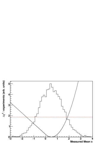
Figure 1: Example set of 5000 toy experiments drawn from $G(\mu=0.5,\sigma=1)$ (histogram), together with the likelihood ratio following Eq. 6 computed in presence of a boundary $\mu>0$ (solid line), and the value $\Delta\chi^{2}_{c}$ giving $\alpha=90\%$ (dashed line).

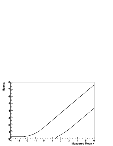
Figure 2: Confidence belt for a unit Gaussian with a mean bound to be positive, $\alpha=90\%$.

For illustration, we compute confidence belts for three additional similar situations: 90% CL without boundaries, 90% CL with a two-sided boundary $0<\mu<3$, and 68% CL with a boundary at $\mu>0$. The previous example of Fig. 2 is repeated for comparison.

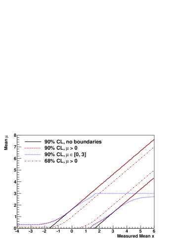
Figure 3: Additional example confidence belts for a unit Gaussian.

III 1–CL plots

Confidence belts might not always be the most convenient way to display information about the statistical precision of a measurement. For instance, if we performed not only one measurement of the above Gaussian mean, the belt becomes a multi-dimensional object. Instead, one often choses to show “$1-\rm CL$” plots for a parameter of interest. An example is given in Fig. 4. These plots display confidence regions for all possible confidence levels, evaluated for one specific (the observed) measured value $x_{0}$. To read off the, say, 68% CL interval $[\mu_{1},\mu_{2}]$ one draws a horizontal line at $1-\rm CL=1-0.68=0.32$. The interval is given by the intersection of this line and the curve. At the most probable value for the true parameter the curves raises to one.

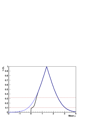
Figure 4: Plot of $1-\rm CL$ of a unit Gaussian for a measured mean of $x=1.4$, both without boundaries (dashed) and for a boundary at $\mu>0$ (solid). The horizontal lines indicate $\alpha=68\%$ and $\alpha=90\%$.

The $1-\rm CL$ plots are constructed using a slight variation of the original toy MC method described above. Steps 1 and 2 remain unchanged:

1. At the considered value of the true parameter $\mu_{0}$, generate a toy experiment.

2. Compute $\Delta\chi^{2}_{\rm toy}\equiv\Delta\chi^{2}(x_{\rm toy},\mu_{0})$ for the toy experiment.

3. Compute $\Delta\chi^{2}_{\rm data}\equiv\Delta\chi^{2}(x_{0},\mu_{0})$ for the measured value.

4. The $1-\rm CL$ ($\equiv 1-\alpha(\mu_{0})$) value is given by the fraction of toy experiments that have a larger $\Delta\chi^{2}$ than the measured value:

   $$1-\alpha(\mu_{0})=\frac{N(\Delta\chi^{2}_{\rm data}<\Delta\chi^{2}_{\rm toy})}{N_{\rm toy}}~{}.$$ (7)

The full $1-\rm CL$ curve is then obtained by scanning for each possible value $\mu_{0}$. The equivalence to the original algorithm can be seen as follows. The confidence interval of coverage $\alpha_{0}$ for the true parameter $\mu$ computed by the $1-\rm CL$ algorithm is given by

$$I_{\mu}=\left\{\mu\>\middle|\>1-\alpha(\mu_{0})>1-\alpha_{0}\right\}~{}.$$ (8)

In step 3 of the original algorithm we have defined $\Delta\chi^{2}_{c}$ such that $\alpha_{0}$ of the toy experiments have smaller $\Delta\chi^{2}$ values, thus we can replace both sides of the inequality,

$$\frac{N(\Delta\chi^{2}(x_{0},\mu)<\Delta\chi^{2}_{\rm toy})}{N_{\rm toy}}>\frac{N(\Delta\chi^{2}_{c}<\Delta\chi^{2}_{\rm toy})}{N_{\rm toy}}~{},$$ (9)

leading to

$$I_{\mu}=\left\{\mu\>\middle|\>\Delta\chi^{2}(x_{0},\mu)<\Delta\chi^{2}_{c}\right\}~{}.$$ (10)

Due to the Neyman construction of the confidence belt both horizontal and vertical intersections of the belt give intervals of coverage $\alpha_{0}$. Thus it is also

$$I_{x}=\left\{x\>\middle|\>\Delta\chi^{2}(x,\mu_{0})<\Delta\chi^{2}_{c}\right\}~{},$$ (11)

which is just the definition of step 4 of the original algorithm.

Two example physics analyses where this method is used can be found in Refs. babarGLW ; babarGGSZ .

IV Two-dimensional CL contours

It is straight-forward to apply the toy MC method to a two-dimensional situation. If there are two, possibly correlated true parameters that shall be estimated from the data, the $1-\rm CL$ plots become three-dimensional. From those, CL contours are readily obtained by slicing at the desired confidence level $1-\alpha_{0}$.

We use the toy MC method to obtain CL contours for the means $\mu_{1}$ and $\mu_{2}$ of a two-dimensional Gaussian. We chose the corresponding widths $\sigma_{1,2}$ different from each other, and also a non-zero correlation. The resulting contours are tilted ellipses. They are shown in Fig. 5 (solid lines). The innermost ellipsis has the property, that its projections onto the $\mu_{1,2}$ axes are exactly $\pm\sigma_{1,2}$. Its confidence level is $\alpha_{0}=39.3\%$.

We also consider the effect of boundaries for the true parameters $\mu_{1,2}$. In Fig. 5 (dashed lines), we chose the allowed region to coincide with the displayed region. The resulting contours all cover a smaller area compared to the unconstrained case: The boundaries seem to “deflect” the contour, resulting in “squeezed ellipses”.

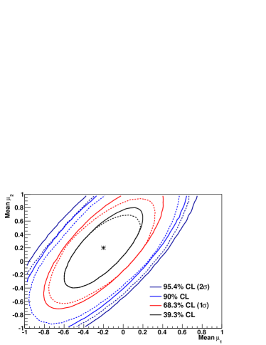
Figure 5: Confidence regions for the mean of a two-dimensional Gaussian with $\sigma_{1}=0.4$, $\sigma_{2}=0.6$, $\rho=70\%$, for a measured mean of $(x_{1},x_{2})=(-0.2,0.2)$ (data point) with coverage $\alpha=39.3\%$, 68.3%, 90%, 95.4% (solid lines from inner to outer). The dashed lines show the corresponding regions in presence of the boundaries $|\mu_{1}|<1$ and $|\mu_{2}|<1$.

V Prob method

In many cases, the likelihood function assumes a Gaussian shape. This is likely the case, when the parameter of interest is itself an estimator that is based on a sufficiently large data sample. Then, $\Delta\chi^{2}$ follows a $\chi^{2}$ distribution with one degree of freedom by definition–which also justifies the use of the symbol in the above. It is therefore possible to compute $1-\rm CL$ from the cumulative distribution function of the $\chi^{2}$ distribution (compare to Eq. 7):

$$1-{\rm CL} =\int_{\Delta\chi^{2}_{\rm data}}^{\infty}P_{\chi^{2}}(t)\,{\rm d}t$$ (12)

$$=\frac{1}{\sqrt{2}\,\Gamma(1/2)}\int_{\Delta\chi^{2}_{\rm data}}^{\infty}t^{-1/2}e^{-t/2}\,{\rm d}t$$ (13)

$$=\textsc{Prob}(\Delta\chi^{2}_{\rm data},1)~{}.$$ (14)

With this approach there is no need for toy MC. The algorithm in Section III just reduces to steps 3 and 4, where in the latter the toy MC ratio is replaced by Eq. 14. The Prob function is available within the Root framework as TMath::Prob().

It should be stated clearly that this method only applies in the Gaussian regime. For instance, it does not handle the presence of boundaries in a satisfactory way. Applied to the situation of Fig. 4 it produces a curve that coincides with the unconstrained F.-C. curve everywhere: When reaching the boundary $\mu=0$, it suddenly drops off to zero. In this situation, correct coverage is not guaranteed.

The clear advantage of the Prob method is that the required amount of computation is very reasonable, as no toy MC generation is involved. And often it gives a very good idea of the F.-C. confidence contours, so it may be instructive to try it before a F.-C. analysis is performed.

VI Conclusion

In their original publication, Feldman and Cousins include a recipe to perform a toy MC computation of their confidence regions. In this note, we explain it in an algorithmic way, that is suited to direct implementation into existing fitter frameworks. We show the connection of the toy MC method to the frequentist confidence belt and to $1-\rm CL$ plots. We illustrate the method using simple one- and two-dimensional Gaussian situations with and without boundaries on their true parameters.

VII Acknowledgements

The author wishes to thank Giovanni Marchiori and Klaus Wacker for useful discussion.

References

- (1) G. J. Feldman and R. D. Cousins, Phys.Rev. D57, 3873 (1998), arXiv:physics/9711021.
- (2) B. D. Yabsley, (2006), arXiv:hep-ex/0604055.
- (3) Particle Data Group, K. Nakamura et al., J.Phys.G G37, 075021 (2010).
- (4) BABAR Collaboration, P. del Amo Sanchez et al., Phys. Rev. D82, 072004 (2010), arXiv:1007.0504.
- (5) BABAR Collaboration, P. del Amo Sanchez et al., Phys.Rev.Lett. 105, 121801 (2010), arXiv:1005.1096.