Hangzhou, 310027, P. R. China
On Primary Relations at Tree-level in String Theory and Field Theory
Abstract
By the use of cyclic symmetry, KK relations and BCJ relations, one can reduce the number of independent -point color-ordered tree amplitudes in gauge theory and string theory from to . In this paper, we investigate these relations at tree-level in both string theory and field theory. We will show that there are two primary relations. All other relations can be generated by the primary relations. In string theory, the primary relations can be chosen as cyclic symmetry as well as either the fundamental KK relation or the fundamental BCJ relation. In field theory, the primary relations can only be chosen as cyclic symmetry and the fundamental BCJ relation. We will further show a kind of more general relation which can also be generated by the primary relations. The general formula of the explicit minimal-basis expansions for color-ordered open string tree amplitudes will be given and proven in this paper.
Keywords:
Gauge symmetry, QCD1 Introduction
The relations among scattering amplitudes play an important role in understanding gauge field theory and quantum gravity. In gauge field theory, color-ordered amplitudes at tree-level have been shown to satisfy many relations. These relations provide constraints on amplitudes. With these relations, one can expand any -point color-ordered tree amplitude by a minimal-basis of amplitudes. The first relation is the cyclic symmetry with which one can reduce the number of independent amplitudes from to . The second one is the Kleiss-Kuijf relationKleiss:1988ne (KK relation). With the KK relations, one can express the amplitudes by only independent amplitudes. The coefficients in front of the amplitudes in cyclic symmetry and KK relations are independent of kinematical factors . The third one is the Bern-Carrasco-Johansson relationBern:2008qj (BCJ relation), with which the number of independent amplitudes can be further reduced down to . Being different from the cyclic symmetry and the KK relations, BCJ relations are highly nontrivial relations, i.e., the coefficients of the amplitudes in BCJ relations are functions of kinematic factors . In quantum gravity, there are Kawai-Lewellen-Tye(KLT) relationsKawai:1985xq that express graviton amplitudes in terms of products of two gluon amplitudes. As in the BCJ relations, there are also nontrivial coefficients in the KLT relations.
All these amplitude relations have been studied in both field theory and string theory. In string theory, the cyclic symmetry is resulted by worldsheet conformal symmetry. Both KK and BCJ relations come from the so-called monodromy relations which can be derived by deforming the contour of worldsheet integralsBjerrumBohr:2009rd ; Stieberger:2009hq ; BjerrumBohr:2010zs . KK relations are the real part relations, while BCJ relations are the imaginary part relations. KLT relations are also monodromy relationsKawai:1985xq ; BjerrumBohr:2010hn . Though the coefficients of the amplitudes in KK relations in field theory are trivial, we should notice that these coefficients in KK relations in string theory are nontrivial functions(cosine functions) of kinematic factors. Thus, in string theory, the only relation with trivial coefficients is the cyclic symmetry.
After taking the field theory limits from string theory, we get the amplitude relations in field theory. However, for the consideration of consistency, pure field theory proofs are also necessary. In field theory, the KK relations were first proven via new color decompositionDelDuca:1999rs , while the fundamental BCJ relations were proven in Feng:2010my ; Jia:2010nz by using BCFW recursionBritto:2004ap ; Britto:2005fq 222 In Tye:2010kg , BCJ relations were considered by using Schouten identity.. In Feng:2010my ; Jia:2010nz , it was stated that one can use a set of fundamental BCJ relations to solve the minimal-basis expansion out. But it seems impossible to prove the general formula of explicit minimal-basis expansionBern:2008qj in this way. This is because the coefficients before the amplitudes are too complicated. The general formula of explicit minimal-basis expansion in field theory was proven in Chen:2011jx via a set of relations called general BCJ relations which are field theory limits of the BCJ relations in string theory(See BjerrumBohr:2009rd ). KLT relations in field theory have been proven in BjerrumBohr:2010ta ; BjerrumBohr:2010zb ; BjerrumBohr:2010yc ; Feng:2010br by BCFW recursion. BCJ relations play an important role in the field theory proof of the KLT relations.
Another representation of BCJ relation is referred as Jacobi-like identity among the kinematic numerators Bern:2008qj . Works in this representation can be found in, e.g., Bern:2010ue ; Bern:2010yg . Recent researches on BCJ numerator can be found in Mafra:2011kj ; Monteiro:2011pc . The relations in heterotic string theory was studied in Tye:2010dd . Many works on amplitude relations via pure spinor string can be found inMafra:2009bz ; Mafra:2010gj , Mafra:2011kj , Mafra:2011nv ; Mafra:2011nw . It is interesting that the KK and BCJ relations are not only hold in gauge field theory but also in other cases, e.g., the KK relations also hold for amplitudes with gluons coupled to gravitonsChen:2010ct , while the BCJ relations were also suggested to be hold for gluons coupled to mattersSondergaard:2009za . In Du:2011js , the KK and BCJ relations in color dressed scalar theory were proven by BCFW recursion with nontrivial boundary Feng:2009ei ; Feng:2010ku . KLT relations are also extensive relations and can be used in many casesBern:1999bx . The KLT relations for pure gauge amplitudes are proven in Du:2011js . The extension of the amplitude relations to loop-level can be found in Bern:2010ue ; Bern:2010yg ; BjerrumBohr:2011xe ; Feng:2011fja . A dual formula of color decomposition was proposed in Bern:2011ia .
Although there have been a lot of studies on amplitude relations, there is an important thing that should be emphasized: The general BCJ relations which were used to prove the minimal-basis expansion in Du:2011js are redundant ones if we consider the fundamental BCJ relations as the primary relations. This is because the minimal-basis expansion is the solution of the general BCJ relationsChen:2011jx and it can also be solved out from a set of fundamental BCJ relationsFeng:2010my ; Jia:2010nz . It is not apparent to extend this statement to the KK relations in field theory. Can we also generate KK relations by some primary relations? If we consider all the cyclic symmetry, KK relations and BCJ relations together, we have a further question: Can we generate all these relations by some primary relations? In fact, as we have mentioned above, in string theory, both KK and BCJ relations come from monodromy. Since they are just the real part and imaginary part of the same monodromy relation, they have fairly equal status in string theory. Thus we speculate that the KK relations can also be generated by some primary relations. In this paper, we will treat all the cyclic symmetry, KK and BCJ relations together. We will show that all these relations in string theory can be generated by two primary relations. One primary relation is the cyclic symmetry while the other one can be chosen as either the fundamental KK relation or the fundamental BCJ relation. This argument can be extended to field theory. In field theory, all the KK and BCJ relations can be generated by the fundamental BCJ relation and the cyclic symmetry. The difference from the string theory case is that the primary relations cannot be chosen as the -decoupling identity(field theory limit of fundamental KK relation in string theory) in field theory. The discussions in string theory can be achieved by the following steps(See (4)):
| (4) | |||
| (7) |
Firstly, we will write the KK and the BCJ relations in string theory into the monodromy relations named KK-BCJ relations. The simplest KK-BCJ relation is the -like decoupling identity(the real part gives the fundamental KK relation, while the imaginary part gives the fundamental BCJ relation). Secondly, we will show that the fundamental KK(BCJ) relation can be generated by the cyclic symmetry and the fundamental BCJ(KK) relation. Thus we can choose the cyclic symmetry as well as either one of the fundamental KK relation and the fundamental BCJ relation as the primary relations to generate the -like decoupling identity. Thirdly, we will generate a kind of relation named generalized -like decoupling identity333The generalized -decoupling identity in field theory was given in Du:2011js . This relation is just the field theory limit of the real part of the generalized -like decoupling identity in this paper. by using the -like decoupling identity. At last, we will show the equivalence between generalized -like decoupling identities and KK-BCJ relations. Thus all the KK and BCJ relations can be generated by only two primary relations. The field theory results can be obtained by taking field theory limits carefully.
In our discussions of this paper, various linear combinations of amplitudes accompanied by momentum kernels are useful. We will use the linear combinations of amplitudes to give a kind of more general relation which is mentioned as general monodromy relation in this paper. The generalized -like decoupling identities and the KK-BCJ relations can be considered as special cases of this kind of relation. The general monodromy relations can also be generated by the primary relations. After taking the field theory limits, we get the corresponding relations in field theory.
As we have mentioned above, the minimal-basis expansion at tree-level for color-ordered amplitudes can be solved from the fundamental BCJ relations Feng:2010my ; Jia:2010nz , but it seems impossible to give the general formula in this way. Though the general formula of minimal-basis expansion for color-ordered pure-gluon tree amplitudes in field theory has been conjectured in Bern:2008qj and proven in Chen:2011jx , the corresponding expression has not been found in string theory. In this paper, we will derive the explicit minimal-basis expansion for color-ordered open string tree amplitudes.
The structure of this paper is as follows. In section 2, we will give a new defined momentum kernel which will be useful in this paper. We will rewrite the monodromy relations by momentum kernels and show an -formula of the color decomposition for open string tree amplitudes via KK-BCJ relation. In section 3, we will show all the KK and BCJ relations can be generated by the primary relations. In section 4, we will extend the combination of amplitudes to give the general monodromy relation. In section 5, we will derive the minimal-basis expansion for color-ordered open string tree amplitudes. A summary of our conclusion will be given in section 6.
2 A new defined momentum kernel and the -formula of color decomposition in string theory
Momentum kernel has been suggested in BjerrumBohr:2010hn and it plays an important role in understanding monodromy relations. In this section, we will give discussions on a new defined momentum kernel which will be useful in this paper. In subsection 2.1, we will provide the definition and useful properties of this momentum kernel. By the use of this momentum kernel we will rewrite the monodromy relations in string theory.
Using the new defined momentum kernel in string theory, one can express the KK and BCJ relations in a complex formula(KK-BCJ relations). With this formula, any amplitude can be expressed as a linear combination of KK basis accompanied by appropriate complex momentum kernels. Thus we expect that there is also an -formula of color decomposition in string theory as in the case of field theoryDelDuca:1999rs . In subsection 2.2, we will show the -formula of color decomposition in string theory by a new defined commutator.
2.1 A new defined momentum kernel in string theory
In this paper, the momentum kernel is defined as
| (8) |
where
| (11) |
Here, and are two permutations of the external legs. We denote the external leg at the -th location in a given permutation as . If for some external leg , we can denote as . For example, in the permutation , we have , and . The momentum kernel is defined as a phase factor which depends on the relative orderings of the legs in two sets and . We take some momentum kernels with three legs as examples
From the definition and the above examples, we can see if the relative orderings of two legs and are different in the two permutations and , this momentum kernel gets a factor . Else, if the relative orderings of two legs in and are same, the momentum kernel only gets a trivial factor . For any two legs, we have a factor or . After considering all the relative orderings in the two permutations, we get the whole momentum kernel. The following properties of the momentum kernel will be useful in this paper:
(i) If the two permutations are identical, we have
| (12) |
(ii) The momentum kernel is symmetric under
| (13) |
(iii) For a given permutation which satisfies , i.e., is a permutation preserving the relative ordering of ,,…,, we have
| (14) | |||||
(iv) For a given , we have
| (15) | |||||
(v) The factorization relation: if , we have
| (16) |
where , , , denote the permutations , , , . denotes the relative orderings of elements come from and .
With the definition of momentum kernel (8), we can write down the monodromy relations in string theory. The general formula of KK-BCJ relationBjerrumBohr:2009rd for color-ordered open string tree amplitudes can be written as
| (17) |
where we use to denote the color-ordered open string tree amplitudes and use to denote the revised ordering of legs in permutation . When taking the real part of the above equation, we get the KK relations. The imaginary part of amplitudes must vanish. Thus, when taking the imaginary part of the above equation, we get a set of constraints on the KK-basis. These constraints are nothing but BCJ relations. As in the case of pure KK relations, the KK-BCJ relations(17) also express any amplitude by amplitudes explicitly. However, in this case, the coefficients of amplitudes are complex ones. The further reductions given by BCJ relations are implied by the vanishing of the imaginary parts of amplitudes. If there is only one element in , (17) becomes
| (18) | |||||
We call it -like decoupling identity444We will see in the next subsection, this is not a real -decoupling identity. However, with the new defined commutator in the next subsection, this identity can be understood similarly as in the case of -decoupling identity in field theory.. The real part of this identity is the fundamental KK relation(its field theory limit gives the -decoupling identity in field theory)
| (19) | |||||
The imaginary part of the -like decoupling identity (18) gives the fundamental BCJ relation(its field theory limit gives fundamental BCJ relation in field theory)
| (20) | |||||
Another kind of useful monodromy relation that will be proven and used in the next section is the generalized -like decoupling identity
| (21) |
It is easy to see that the fundamental -like decoupling identity(18) is the special case of the above equation with only one .
Both the KK-BCJ relation and the generalized -like decoupling identity can be considered as the special cases of the following general monodromy relation
| (22) | |||||
where the is the complex conjugate of . In fact, if there is no element in , the above equation becomes KK-BCJ relations(17). If there is no element in , the above equation becomes the complex conjugates of generalized -like decoupling identities(21). The general monodromy relations will be derived in section 4.
With this definition of momentum kernel, we can also write down KLT relations(See Eq. (1.1) in Kawai:1985xq ) directly
| (23) |
where denote closed string tree amplitude. In the KLT relations (23) each open string takes half of the momentum of the corresponding closed string.
2.2 The -formula of color decomposition in string theory
In field theory, one can express the total -gluon amplitudes at tree-level by either the standard color decomposition with color-ordered amplitudes or the color decomposition with color-ordered amplitudes(KK basis) Del Duca:1999ha , DelDuca:1999rs . This is because the amplitudes in the standard color decomposition can be expressed by KK basis. In string theory, when we introduce the gauge degree of freedom by adding Chan-Paton factors to the ends of open strings, the total amplitudes at tree-level for open strings can also be given by the standard color decomposition
| (24) |
However, as we have mentioned, there are nontrivial kinematic factors before the amplitudes in the KK relations in string theory. Thus the -formula of color decomposition in string theory should be reconsidered. In this subsection, we will show that the -formula of color decomposition in string theory can be given as
| (25) |
Here the commutator is defined as
| (26) |
In this new defined commutator, there is a factor that depends on kinematic factor . The momentum of a commutator is defined as . After taking the field theory limits, we get the ordinary commutators in field theory and the color decomposition becomes the one expressed by KK basis in field theoryDelDuca:1999rs .
It is interesting that if there is some commute with all the other ones in this new defined commutator, from the standard color decomposition (24), we obtain the relation (18). This is similar with the -decoupling identity in field theory, but the commutators used are the new defined ones in which there are kinematic factors. That’s why we call (18) -like decoupling identity. The generalized -like decoupling identities (21) can be considered as the extensions of -like decoupling identity (18) 555This is similar within the field theory caseDu:2011js .. Before giving the general discussion on this -formula of color decomposition, we first give an example.
2.2.1 Example
We now take the four-point amplitude as an example. If (25) gives the right color decomposition with KK basis, we can transform (25) to the standard color decomposition (24) by using KK-BCJ relation (17)(which express the amplitudes by amplitudes) 666We can also use only KK relations(real part), however, in this paper, we use the KK-BCJ relations. One thing should be further noticed is that the imaginary parts of amplitudes must vanish..
The total four-point amplitude can be expressed by (25)
| (27) |
Expanding the new defined commutators in the traces, we get
| (28) | |||||
Now we collect the terms containing a same trace, e.g., for the trace , we only have , while for the trace , both the two permutations , , , and , , , contribute to this trace because we have and , we thus have
| (29) |
When we consider the KK-BCJ relation with , , the above expression becomes . In a similar way, for any given trace, we can collect all the terms containing this trace and use an appropriate KK-BCJ relation to get an amplitude which has a same ordering within the trace. After considering all the traces, we get the standard color decomposition
| (30) | |||||
Thus the color decomposition (27) is equivalent with the standard color decomposition.
2.2.2 General discussion
The discussion in the above example can be extended to the general proof. In general, for a given , we have a trace of the form
| (31) |
When we expand the commutators in this trace, we get terms. In each term, there is a trace of the form
| (32) |
This trace is accompanied by a phase factor when we consider the definition of momentum kernel (8)
| (33) |
Any given can split into two ordered sets and , where the relative orderings of the legs in each ordered set are same with those in the permutation . For a given , there are such splittings corresponding to the traces(we should notice that in the trace, the relative ordering of ,…, is the reversed ordering of ,…, in ). Thus the total amplitude should be expressed as
| (34) | |||||
Because we sum over all permutations , all the permutations must be included. Thus, for a given trace , we can collect all the permutations which can split into two ordered sets and . We get
| (35) |
where we have used KK-BCJ relations. The ordering of the legs in is same with the ordering of the s in the trace. After considering all the traces with different s, we get the standard color decomposition (24).
3 Generating KK and BCJ relations by primary relations
As we have mentioned in the introduction, one can use the amplitude relations including the cyclic symmetry, KK and BCJ relations to reduce the number of the independent -point color-ordered amplitudes from down to . It is interesting that all the BCJ relations can be solved from a set of fundamental BCJ relations. In this section, we will consider the question: When we consider all the cyclic symmetry, KK and BCJ relations together, can we generate all these relations by some primary relations? We will show that among all these relations, there are two primary relations. All other relations can be generated by the two primary relations. In string theory, one primary relation is the cyclic symmetry, while the other one can be chosen as either one of fundamental KK relation and fundamental BCJ relation. However, in field theory, if we do not consider the higher-order corrections, the fundamental KK relation(i.e., -decoupling identity in field theory) cannot be chosen as a primary relation. We can only choose the cyclic symmetry and the fundamental BCJ relation as the primary relations. This is because the kinematic factors which is necessary to generate BCJ relations do not appear in the -decoupling identity in field theory.
In the following subsections we will first show how to generate -like decoupling identity (18) by two primary relations. Then we will show the generalized -like decoupling identities (21) can be generated by -like decoupling identities (18). After that, we will show the equivalence between generalized -like decoupling identities (21) and KK-BCJ relations (17). Thus all the KK and BCJ relations can be generated by the primary relations. We then will take the field theory limits to show how to generate all KK and BCJ relations in field theory.
3.1 Generating -like decoupling identity by primary relations
In this section, we will show if we know either the fundamental KK relation or fundamental BCJ relation, we can generate the other one(then the whole -like decoupling identity) by using cyclic symmetry. This means only two relations are the primary relations. The two primary relations can be chosen as the cyclic symmetry
| (36) |
and arbitrary one of fundamental KK relation (19) and fundamental BCJ relation (20).
Before our discussions, we should emphasize one thing. The -like decoupling identity (18) can be understood as follows: We move from the first location in the amplitude to the -th location. When we move from the left side to the right side of , we get a phase factor multiplied to the corresponding amplitude. After consider all different locations of , we get the -like decoupling identity (18). If the starting point of is not the first location, e.g., the starting point is the second location, we have another -like decoupling identity
| (37) |
This -like decoupling identity can be obtained by multiplying a phase factor to both sides of (18) (Here the momentum conservation and on-shell condition should be considered). Thus the -like decoupling identities with different starting points of are equivalent relations. If we know the -like decoupling identity with one starting point of (e.g.,), we know all the -like decoupling identities (thus the fundamental KK and fundamental BCJ relations) with other starting points of . In the following subsection, we will show that the -like decoupling identity (18) can be generated by two primary relations.
3.1.1 Fundamental BCJ relation and cyclic symmetry as the primary relations
The fundamental KK relation (19) is not an independent relation if we consider the fundamental BCJ relation(20) and the cyclic symmetry(36) as the primary ones. This is because any amplitude in the fundamental BCJ relation (20) has the cyclic symmetry (36) and we can use the cyclic symmetry to change the starting point of the leg from the second location to the third location to get another equivalent fundamental BCJ relation. Combining the two fundamental BCJ relations appropriately, we can derive the real part condition(the fundamental KK relation) (19). We now show the details.
When we consider the amplitudes with as the first leg, according to the fundamental BCJ relation (20) with the starting point of at the second location, we have
| (38) | |||||
With the cyclic symmetry (36), this relation turns to an equivalent relation with the starting point of at the third location
| (39) | |||||
Using , the cyclic symmetry (36), the fundamental BCJ relation(20), momentum conservation, the on-shell conditions and (e.g., in 26-dimensional bosonic string theory, for tachyon for massless vector , in 10-dimensional superstring theory, for massless vector ), the relation (39) can be rewritten as
| (40) | |||||
This just gives the fundamental KK relation (19). Thus we have derived the fundamental KK relation by using the fundamental BCJ relation and cyclic symmetry as the primary relations.
3.1.2 Fundamental KK relation and cyclic symmetry as the primary relations
We can also consider the fundamental KK relation (19) and the cyclic symmetry (36) as the primary relations. In this case, the fundamental BCJ relation (20) can be generated. Actually, as what we have shown in the previous subsection, using the cyclic symmetry, we can also move the starting point of in (19) from the first location to the second location
| (41) | |||||
Using , the momentum conservation, the cyclic symmetry (36) the on-shell conditions and the fundamental KK relation(19), the above equation becomes
| (42) | |||||
This is just the fundamental BCJ relation (20). So we have shown that the fundamental KK relation and the cyclic symmetry can also be considered as the primary relations. With this choice of primary relations, the fundamental BCJ relation can be generated.
3.2 Generating generalized -like decoupling identity by -like decoupling identity
In previous subsection, we have seen that -like decoupling identity can be generated by two primary relations. In this subsection, we will show the generalized -like decoupling identities (21) with more s is redundant relation, i.e., they can be generated by the -like decoupling identity (18).
To see this, we write the L. H. S. of (21) as
| (43) |
To show (21) with s(we mention it as level- relation) can be generated by the -like decoupling identity, we will show can be given as linear combinations of those s with s fewer than . Then we get a recursive relation. The starting point of this recursion is the -like decoupling identity (18). Once the -like decoupling identity (18) holds, the generalized -like decoupling identities (21) with more than one s must also hold.
It will be convenience for us to introduce the following linear combinations
| (44) |
where is defined by (43). has other two useful forms which can be obtained from (44), (43) and the factorization property of momentum kernels (16). One is
| (45) |
The other one is
| (46) |
It is worth to point that the following recursive relation will be useful. If
| (47) |
where can be any integer satisfying , we can express for any by and
| (48) |
This recursion relation will be used again and again in this paper.
To make the recursive construction more clearly, we first give some examples.
3.2.1 Examples
We now give some warm-up examples.
Level-1
The first example is the relation with only one . This is nothing but the -like decoupling identity
| (49) |
Level-2
In the case with two s, we consider the following three linear combinations (44) with and distributed into the ordered sets and in (44). The first one is
| (50) | |||||
When we move into the ordered set , we get the second one
| (51) | |||||
where we have used (46). When we further move into the ordered set , the ordered set then becomes empty, while the set has two elements with the relative ordering , . In this case we get the third one
| (52) | |||||
where the property of momentum kernel (14) has been used in the last line. If we define
| (53) |
the relation (47) is satisfied for . Thus (48) gives
| (54) |
Exchanging and , we have another equation
| (55) |
From the two equations above, we get
Using the definition of (44), can be expressed as
| (57) |
while can be expressed as
| (58) |
Once we have -like decoupling identity, and must vanish, then also vanishes. Hence all the level-2 generalized -like decoupling identities are generated by the -like decoupling identity (18).
Level-3
Now let us consider the level-3 relation. In this case, we should distribute , into the two ordered sets and in (44). We just use those combinations with keeping the relative orderings in the permutation , , in each ordered set, i.e., , , and . Each one can be given by the expression (46). In (46), the first element in can be either the first one in or the first one in . Thus we can rewrite these combinations of amplitudes as
| (59) | |||||
| (60) | |||||
| (61) | |||||
| (62) | |||||
We should notice that the in (62) is same with that in the second term of (61), the in the first term of (61) is same with that in the second term of (60) while the in the first term of (60) is same with that in (59). Using (44) to adjust the coefficients in each equation, we can define
| (63) |
These s and s satisfy (47), thus they also satisfy (48). We have
| (64) | |||||
Now we replace , , by , , , i.e., reverse the relative ordering of legs in permutation , , , we get another equation
| (65) | |||||
From this two equations above, we can solve out
| (66) | |||||
Substituting all the s in the above equation by the definition (44), as in case of level-2, we express by those s at level-2 and level-1. Since the -like decoupling identities at level-2 have been generated by the -like decoupling identity, the level-3 identities can also be generated by the -like decoupling identity.
3.2.2 General discussion
The discussions on level-2 and level-3 can be extended to the general case. In general, we can distribute into two ordered sets and for any . We consider this two ordered sets as the sets and in . Then for a given , we have which can be expressed by (46). Noticing the first element in can be either or , we have
For any given and a permutations there exists a identical to , . Thus, for a given , the second term of is proportional to the first term of . Adjusting the coefficients and using the property (14), we can define
| (68) |
These definitions satisfy (47), then from (48) we have
| (69) | |||||
Now we reverse the ordering of , i.e., we do the replacement , we get another equation
| (70) | |||||
can be solved out from the above two equations
| (71) | |||||
From (44) we know and are defined by combinations of s with s fewer than . If the generalized -like decoupling identities at level- can be generated by the -like decoupling identity, the generalized -like decoupling identity at level- can also be generated by the -like decoupling identity.
3.3 Generating KK-BCJ relation by generalized -like decoupling identity
So far, we have shown that all the generalized -like decoupling identities can be generated by -like decoupling identity. In this subsection, let us turn to the KK-BCJ relation(17). We will show the generalized -like decoupling identities and the KK-BCJ relations can be solved from each other, i.e., they are equivalent relations. Thus all the KK-BCJ relations are generated by the primary relations. Since the KK and BCJ relations are just the real part and imaginary part of KK-BCJ relations, they can also be generated by primary relations. To show the equivalence of KK-BCJ relations and generalized -like decoupling identities, we define another useful linear combination of amplitudes by the L. H. S. of KK-BCJ relations (17)
The equivalence between KK-BCJ relation and generalized -like decoupling identity means and can be expressed by each other. We first give some examples.
3.3.1 Examples
In this subsection, we give some examples to show the equivalence between generalized -like decoupling identities and the KK-BCJ relations.
Level-1
In section 2, we have already mentioned that the KK-BCJ relation is same with the generalized -like decoupling identity at level-1. At this level, they all become -like decoupling identity (18), i.e.,
| (73) |
Level-2
Now we consider level-2. The difference between at level-2 and at level-1 is
| (74) | |||||
where we have used the property (14). The last line in the above equation is just multiplied by a factor . Thus we can express the at level-2 by those s at level-2 and level-1
| (75) |
If we define
| (76) |
the relation (47) is satisfied. Thus we can use (48) to express as
| (77) |
This means we can also use the generalized -like decoupling identities at level-2 and level-1 to express the KK-BCJ relation at level-2. Thus the KK-BCJ relations at level-() are equivalent with the generalized -like decoupling identity at level-(). Since we have shown that all the generalized -like decoupling identities can be generated by the primary relations, the KK-BCJ relation at level-2 can also be generated by the primary relations.
level-3
Now let us consider the relations with three s. As in the level-2 case, we have
| (78) | |||||
From this, we can express by and as
| (79) | |||||
We can define
| (80) |
As we have shown in the cases of level-1 and level-2, we can define
| (81) |
Again, we have (47) and then from (48) we can express by the s with not more than threes
| (82) | |||||
Therefore, the KK-BCJ relations with not more than three s are equivalent with the generalized -like decoupling identities with not more than three s. The KK-BCJ relation at level-3 thus can be generated by the primary relations.
3.3.2 General discussion
As what we have shown in the above examples, in general, from the definitions (43), (3.3) and the property of momentum kernel (14), we have
| (83) | |||||
This formula express any by s at level- and level-. To express by s, according to the above equation with no more than s in , we can define
| (84) |
Under this definition of and , the relation (47) is satisfied. Thus according to (48), we have
| (85) | |||||
Since the generalized -like decoupling identities have been generated by the primary relations, the KK-BCJ relations also holds automatically. This tells us all the KK-BCJ relations are generated by the primary relations.
Before we continue this discussions to the field theory limits, we should pay attention to the boundary case. The boundary case of KK-BCJ relations with only one is given as
| (86) |
This is nothing but just the color-order reversed relation
| (87) |
Using momentum conservation, we have
| (88) | |||||
Using on-shell conditions and for , we can give the color-order reversed relation as 777This color-order reversed relations is a little different from the ordinary one . In fact, cyclic symmetry connects this two expressions.
| (89) |
3.4 Field theory limits
We can extend all above discussions in string theory to field theory by taking . After taking the field theory limits, the massless states of open strings are left. We get the relations among pure-gluon amplitudes. Only the leading orders of the real part and the imaginary part contribute to the relations. To write down the field theory limits of the monodromy relations, we should use the momentum kernel
| (90) |
To generate the KK and BCJ relations in field theory by primary relations, we should first express the corresponding KK and BCJ relations in string theory by the primary relations. Then taking field theory limits in the relations. The difference from string theory is that the decoupling identity(fundamental KK relation) cannot be chosen as one of the primary relations in field theory. This is because we need the kinematic factors in BCJ relations in field theory, but in KK relations in string theory, the kinematic factors only come from higher-order terms of the expansion of cosine functions. When taking the field theory limits, we only keep the leading parts of the cosine functions, the kinematic factors are ignored. However, Since there are kinematic factors in the BCJ relations in field theory, we can consider the fundamental BCJ relation and the cyclic symmetry as the primary relations.
Now we consider a five-point example with two s to show the details. The five-point KK relation with two s is given as
| (91) |
where we consider the legs and as the , . Correspondingly, the BCJ relation with two s is given as
| (92) | |||||
We denote the L. H. S. of the KK and BCJ relations in string theory as and respectively. The field theory limits of the L.H.S. of KK and BCJ relations are denoted by and . To show the two relations (91) and (92) can be generated by the fundamental BCJ relation and the cyclic symmetry, we can write this two relations into a complex KK-BCJ relation
| (93) | |||||
To show how to generate this relation by the primary relations, we first express in string theory. Using (77), (3.2.1), (57) and (58), we have
| (94) | |||||
As we have pointed in the subsection (3.1.1), when we consider the fundamental BCJ relation and the cyclic symmetry as the primary relations, we have
| (95) |
where and are the L. H. S. of the fundamental KK and the fundamental BCJ relations respectively. Thus we can express by s with only one as
After taking , we should use and , instead of and respectively.
Expanding both sides of the above equation according to the powers of . We can write down the contributions from different orders in . The first contribution of the above equation may be . In this case, we have
| (97) | |||||
However, using the leading order of (95), the above equation becomes
| (98) |
This contribution vanishes because the first three terms can be obtained by first inserting then inserting at the possible locations while the last three terms can be obtained by first inserting then inserting at the possible the locations. The two kinds of insertion are equivalent. Noticing the first three terms and the last three terms have different signs, they cancel out with each other.
Now we consider the order. In the L. H. S. of (3.4), it is just the leading order of the real part of , i. e., the L. H. S. of field theory KK (91). The R. H. S. of (3.4) then expresses by the fundamental BCJ relations in field theory as
| (99) | |||||
One can check this equation by writing the and the s explicitly in terms of amplitudes. From this equation, we can see, the KK relation with two s is nothing but just a linear combination of the fundamental BCJ relations.
For the order, only has a term which is the leading order of the imaginary part of . Thus from (3.4), we express the as linear combination of L. H. S. of fundamental BCJ relations by collecting the terms in R. H. S. of (3.4)888In the derivation, we encounter the contributions from the phase factors of the form , the coefficients of KK relation and the coefficients of BCJ relation. Since there is the factor , to get contribution of the terms in the braces in(94), we should keep the terms in in the braces. The terms with may come from the expansion of phase factor with , the expansion of the coefficients of KK relation with and the term in the expansion of phase factor multiplied by the term in BCJ relation. Since for each there is a corresponding term of the form . Here is the phase factor, cosine functions are the coefficients in KK relation, sine functions are the coefficients in the BCJ relation, . We can use to write all the tree kinds of contributions by BCJ coefficients. At last, we express by only fundamental BCJ relations.
| (100) | |||||
This can also be checked by writing the s explicitly in terms of amplitudes. This equation expresses the BCJ relation with two s for five-point amplitudes as a linear combination of fundamental BCJ relations. Once we have the fundamental BCJ relation, the BCJ relation with two s holds naturally.
4 General monodromy relation
In the previous section, we have seen the equivalence between the KK-BCJ relations and generalized -like decoupling identities. In this section, we extend this discussion to a more general case. We will give the general monodromy relations(22). To show (22), we define a linear combination of amplitudes as the L. H. S. of (22)
(22) in this definition becomes . This kind of relation can be seen from monodromy and can also be generated by the primary relations. After taking the field theory limits, we can obtain the corresponding relations in field theory.
4.1 Monodromy
Now we will show that (22) is the result of monodromy. To show this, we first return to the monodromy derivation of KK-BCJ relations (17) BjerrumBohr:2009rd ; Stieberger:2009hq ; BjerrumBohr:2010zs . We consider an open string worldsheet integral. In this integral the vertex operators of the legs has the relative ordering for and for , while the vertex operators of legs s has the relative ordering . We have the integral
| (102) | |||||
where for a given is defined as , thus the integrals are written as integrals. In the above equation, we have fixed , the two states and are inserted at and respectively. The operator is defined as
| (103) |
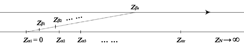
This integral can be expressed by Fig. 1 and it must vanish when we close the contour above the real axis. We consider as a standard integral region, when we break the worldsheet integral into pieces corresponding to different possible permutations of all legs, for a given integral ordering, we can adjust the positions of vertex operators to make the them in the same ordering with the corresponding integrals. Then we get the amplitude with legs in this ordering. Considering the branch point are at the positions of vertex operators, when we move an vertex operator from the left side to the right side of another vertex operator , comparing to the former ordering, the amplitude with legs in the latter ordering should be accompanied by a phase factor . Similarly, if we move from the right side to the left side of another vertex operator , we obtain a phase factor . After considering all the phase factors, The vanishing of the integral (102) gives (17). Particularly, the integral with corresponds to the first term of (17) while the integrals with correspond to the second term of (17).
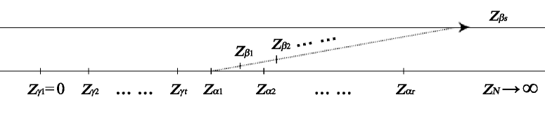
Now we consider another vanishing worldsheet integral
| (104) | |||||
where we have choose the fixed point as , and . The operator is the extension of
| (105) | |||||
Here . This integral can be expressed by Fig. 2. We can break all the integrals (104) into pieces corresponding to all the possible orderings of the legs and adjust the positions of the vertex operators. As pointed in the case of KK-BCJ relation, an appropriate phase factor should be considered when we adjust the positions of the vertex operators. Then for the permutations with the relative ordering , we get the first term of (22), while for the permutations with the relative ordering , we get the second term of (22). Thus we get the general monodromy relations (22). In next subsection, we will see, this general monodromy relations can also be constructed by the primary relations.
4.2 Generating general monodromy relation by primary relations
In this subsection, we will show that the general monodromy relations (22) can also be generated by the primary relations. To see this, we just use the KK-BCJ relations to generate this kind of relation. Since the KK-BCJ relations can be generated by the primary relations, (22) can also be generated by the primary relations.
4.2.1 An example
The boundary case of (22) is . When , there is no , from the definition of , we have
| (106) |
Now let us consider the (22) with .
Level-1
If there is only one , (22) becomes
The first element in the permutation in can be either or . Thus the first term of can be written as (4.2.1)
| (108) | |||||
where (15) has been used.
Similarly, the second element in the permutation in can be either or . Thus we can write down the second term of (4.2.1) as
| (109) | |||||
Considering both two terms, from the definition of , we get
Since the in the boundary case with vanishes, we can express all the s with s by those with s
| (111) |
This gives a recursive relation. With this relation, we can express the with s by the with no
| (112) |
Because we have , using the KK-BCJ relation with one (i.e., the -like decoupling identity), we get the general monodromy relation with only one
| (113) |
4.2.2 General proof
Now we consider the general case with arbitrary number of s. As pointed in the above example, The first element in the permutation in can be either or . Thus the first term of (22) can be expressed as
| (114) | |||||
The second element in the permutation in can be either or . Thus the second term of (22) becomes
| (115) | |||||
As what we have shown in the level-1 case, we have
With this relation, we can relate the s which have s with those have s
If we define
| (118) |
The recursive relation (47) is satisfied again, thus from (48) we can express the s with s by those with s
| (119) | |||||
The s with s and the s with s can be solved from each other, thus they are equivalent relations. Using this recursive relation, we can express all the s by linear combinations of those with no . Since the boundary condition is given as
| (120) |
and the KK-BCJ relation can be generated by the primary relations, the general monodromy relations (22) thus can also be generated by the primary relations. In the following subsection, we will discuss on the field theory limits of the general monodromy relations (22).
4.3 Field theory limits
We can obtain the field theory limits of the general monodromy relations (22) by taking and replacing the definition of momentum kernel by (90). Keeping the leading terms of both the real parts and the imaginary parts of the relations, we get the corresponding relations in field theory.
We just give an example here, when we consider the six-gluon amplitudes with , , and . The in field theory is
| (121) | |||||
The real part of the above relation reads
| (122) |
This relation can be checked when we use KK relations to express , and by the amplitudes with as the first leg and as the last leg. The imaginary part relation is given as
| (123) |
This one can also be checked by using BCJ relations and KK relations. In general, all other relations corresponding to the real parts and the imaginary parts of the general monodromy relations can be given in a similar way. As in the field theory case of the KK and BCJ relations, both the real parts and the imaginary parts of the field theory limits of general monodromy relations can be generated by the fundamental BCJ relations and the cyclic symmetry.
5 The minimal-basis expansion for color-ordered open string disk amplitudes
By the use of cyclic symmetry, KK and BCJ relations, one can reduce the number of independent amplitudes from to . The explicit expression of the minimal-basis expansion which expresses the KK basis by the BCJ basis in field theory was conjectured in Bern:2008qj . It was pointed in Feng:2010my ; Jia:2010nz that the minimal-basis expansion could be solved from a set of fundamental BCJ relations. The conjectured formula Bern:2008qj was proven in Chen:2011jx . However, the explicit minimal-basis expansion in string theory has not been given yet. In this section, we will derive the minimal-basis expansion of color-ordered open string tree amplitudes. The field theory limit of this expression gives the minimal-basis expansion for color-ordered pure-gluon tree amplitudes. In the following derivation, we only use the BCJ relations which are the imaginary relation of KK-BCJ relations (17)
| (124) |
where
| (125) |
We will first show some examples.
5.1 Examples
In this subsection, we will show some examples.
Level-1
If there is only one , we return to the fundamental BCJ relation
Here we have used the permutations in are same with those in .
Level-2
The next example is given as the amplitudes with two s. If there are two s, we have
| (127) | |||||
The amplitudes in the first term can be further expressed by the minimal-basis expansion with only one . Then we have
| (128) | |||||
where . Considering different permutations of and , we can express the above equation by a sum over . If , the second term of the above equation does not contribute to this permutation. The first term of (128) gives
| (129) |
where denotes the permutation of the legs except in .
If , both two terms of (128) contribute to this kind of permutation
| (130) |
Those in two different cases corresponding to different relative orderings of and in can be written together
| (131) | |||||
Level-3
The BCJ relations with three s can be given as
| (132) | |||||
We notice that the second term only contributes to the permutations with the relative ordering , thus we can multiply a theta function to this term and then replace the permutations by . Similarly, we can multiply to the third term and then replace by . Substituting the minimal-basis expansions at level-2 and level-1 into the first and the second term of this equation respectively, we express every term in the above equation by summing over all permutations with the relative ordering of the s preserved
where denotes the permutation of the legs in except the legs ,…, . This is just the minimal-basis expansion with three s.
5.2 General formula
It is easy to extend the discussions in the examples to general formula by induction. In general, we can divide the ordered set into segments, i.e., ordered sets , ,…,. We denote the last element of the th ordered set as . For any given division with segments, we have . We also define and the th set is empty. For such a division with segments, we get a contribution
| (134) |
is defined as
| (137) |
where, the case with means there is only one element . Considering all the possible divisions for any given permutation (), we can give the minimal-basis expansion as
This can be seen from the examples explicitly, e.g., for the case with three s, there are four possible divisions of . The first division is . The second division is , . The third division is and the fourth division is . The contributions to the minimal-basis expansion of this four divisions just corresponds to the four terms in (5.1).
To prove this minimal-basis expansion, we should consider the BCJ relation with s. Using the BCJ relation with s, we obtain
| (139) | |||||
We can multiply to the first term in the brackets and sum over all instead of . In a similar way, we can also multiply to the terms in the second line for any given and use the sum over instead of the sum over . The special case with only gets a trivial factor instead of the products of theta functions. After substituting the minimal-basis expansions with s fewer than , and noticing the definition of , we get
The two sums and means first merge with the ordered set , then merge with . They can be written into only one sum . Since is independent of , it can commute with the sum . We have
Here we sum over , all the sets in the momentum kernel are expressed by modulo a subset of . For example we express by . We can consider the ordered set as the last set in a division of . Different corresponds to the divisions with different number of elements in the last set. Together with the divisions , this gives all the possible divisions of . At last, we get the minimal-basis expansion (5.2).
6 Conclusion
In this paper, we show that there are two primary relations among all the relations for open string tree amplitudes. One of the primary relations can be chosen as the cyclic symmetry, the other one can be chosen as either the fundamental KK relation or the fundamental BCJ relation. In field theory, the primary relations can only be chosen as the fundamental BCJ relation and the cyclic symmetry. We establish a kind of general monodromy relation which can also be generated by the primary relations. The general formula of the explicit minimal-basis expansions for open string tree amplitudes is given in this paper.
Acknowledgements
This work is supported in part by the NSF of China Grant No. 11105118, No. 10775116, No. 11075138, and 973-Program Grant No. 2005CB724508.
References
- (1) R. Kleiss and H. Kuijf, “MULTI - GLUON CROSS-SECTIONS AND FIVE JET PRODUCTION AT HADRON COLLIDERS,” Nucl. Phys. B 312 (1989) 616.
- (2) Z. Bern, J. J. M. Carrasco and H. Johansson, “New Relations for Gauge-Theory Amplitudes,” Phys. Rev. D 78 (2008) 085011 [arXiv:0805.3993 [hep-ph]].
- (3) H. Kawai, D. C. Lewellen and S. H. H. Tye, “A Relation Between Tree Amplitudes of Closed and Open Strings,” Nucl. Phys. B 269 (1986) 1.
- (4) N. E. J. Bjerrum-Bohr, P. H. Damgaard and P. Vanhove, “Minimal Basis for Gauge Theory Amplitudes,” Phys. Rev. Lett. 103 (2009) 161602 [arXiv:0907.1425 [hep-th]].
- (5) S. Stieberger, “Open & Closed vs. Pure Open String Disk Amplitudes,” arXiv:0907.2211 [hep-th].
- (6) N. E. J. Bjerrum-Bohr, P. H. Damgaard, T. Sondergaard and P. Vanhove, “Monodromy and Jacobi-like Relations for Color-Ordered Amplitudes,” JHEP 1006 (2010) 003 [arXiv:1003.2403 [hep-th]].
- (7) N. E. J. Bjerrum-Bohr, P. H. Damgaard, T. Sondergaard and P. Vanhove, “The Momentum Kernel of Gauge and Gravity Theories,” JHEP 1101 (2011) 001 [arXiv:1010.3933 [hep-th]].
- (8) V. Del Duca, L. J. Dixon and F. Maltoni, “New color decompositions for gauge amplitudes at tree and loop level,” Nucl. Phys. B 571 (2000) 51 [arXiv:hep-ph/9910563].
- (9) B. Feng, R. Huang and Y. Jia, “Gauge Amplitude Identities by On-shell Recursion Relation in S-matrix Program,” Phys. Lett. B 695 (2011) 350 [arXiv:1004.3417 [hep-th]].
- (10) Y. Jia, R. Huang and C. Y. Liu, “-decoupling, KK and BCJ relations in SYM,” Phys. Rev. D 82 (2010) 065001 [arXiv:1005.1821 [hep-th]].
- (11) R. Britto, F. Cachazo and B. Feng, “New recursion relations for tree amplitudes of gluons,” Nucl. Phys. B 715 (2005) 499 [arXiv:hep-th/0412308].
- (12) R. Britto, F. Cachazo, B. Feng and E. Witten, “Direct proof of tree-level recursion relation in Yang-Mills theory,” Phys. Rev. Lett. 94 (2005) 181602 [arXiv:hep-th/0501052].
- (13) H. Tye and Y. Zhang, “Comment on the Identities of the Gluon Tree Amplitudes,” arXiv:1007.0597 [hep-th].
- (14) Y. X. Chen, Y. J. Du and B. Feng, “A Proof of the Explicit Minimal-basis Expansion of Tree Amplitudes in Gauge Field Theory,” JHEP 1102 (2011) 112 [arXiv:1101.0009 [hep-th]].
- (15) N. E. J. Bjerrum-Bohr, P. H. Damgaard, B. Feng and T. Sondergaard, “Gravity and Yang-Mills Amplitude Relations,” Phys. Rev. D 82 (2010) 107702 [arXiv:1005.4367 [hep-th]].
- (16) N. E. J. Bjerrum-Bohr, P. H. Damgaard, B. Feng and T. Sondergaard, “New Identities among Gauge Theory Amplitudes,” Phys. Lett. B 691 (2010) 268 [arXiv:1006.3214 [hep-th]].
- (17) N. E. J. Bjerrum-Bohr, P. H. Damgaard, B. Feng and T. Sondergaard, “Proof of Gravity and Yang-Mills Amplitude Relations,” JHEP 1009 (2010) 067 [arXiv:1007.3111 [hep-th]].
- (18) B. Feng and S. He, “KLT and New Relations for N=8 SUGRA and N=4 SYM,” JHEP 1009 (2010) 043 [arXiv:1007.0055 [hep-th]].
- (19) Z. Bern, J. J. M. Carrasco and H. Johansson, “Perturbative Quantum Gravity as a Double Copy of Gauge Theory,” Phys. Rev. Lett. 105 (2010) 061602 [arXiv:1004.0476 [hep-th]].
- (20) Z. Bern, T. Dennen, Y. t. Huang and M. Kiermaier, “Gravity as the Square of Gauge Theory,” Phys. Rev. D 82 (2010) 065003 [arXiv:1004.0693 [hep-th]].
- (21) C. R. Mafra, O. Schlotterer and S. Stieberger, “Explicit BCJ Numerators from Pure Spinors,” arXiv:1104.5224 [hep-th].
- (22) R. Monteiro and D. O’Connell, “The Kinematic Algebra From the Self-Dual Sector,” arXiv:1105.2565 [hep-th].
- (23) S. H. Henry Tye and Y. Zhang, “Dual Identities inside the Gluon and the Graviton Scattering Amplitudes,” JHEP 1006 (2010) 071 [Erratum-ibid. 1104 (2011) 114] [arXiv:1003.1732 [hep-th]].
- (24) C. R. Mafra, “Simplifying the Tree-level Superstring Massless Five-point Amplitude,” JHEP 1001 (2010) 007 [arXiv:0909.5206 [hep-th]].
- (25) C. R. Mafra, O. Schlotterer, S. Stieberger and D. Tsimpis, “Six Open String Disk Amplitude in Pure Spinor Superspace,” Nucl. Phys. B 846 (2011) 359 [arXiv:1011.0994 [hep-th]].
- (26) C. R. Mafra, O. Schlotterer and S. Stieberger, “Complete N-Point Superstring Disk Amplitude I. Pure Spinor Computation,” arXiv:1106.2645 [hep-th].
- (27) C. R. Mafra, O. Schlotterer and S. Stieberger, “Complete N-Point Superstring Disk Amplitude II. Amplitude and Hypergeometric Function Structure,” arXiv:1106.2646 [hep-th].
- (28) Y. X. Chen, Y. J. Du and B. Feng, “On tree amplitudes with gluons coupled to gravitons,” JHEP 1101 (2011) 081 [arXiv:1011.1953 [hep-th]].
- (29) T. Sondergaard, “New Relations for Gauge-Theory Amplitudes with Matter,” Nucl. Phys. B 821 (2009) 417 [arXiv:0903.5453 [hep-th]].
- (30) Y. J. Du, B. Feng and C. H. Fu, “BCJ Relation of Color Scalar Theory and KLT Relation of Gauge Theory,” arXiv:1105.3503 [hep-th].
- (31) B. Feng, J. Wang, Y. Wang and Z. Zhang, “BCFW Recursion Relation with Nonzero Boundary Contribution,” JHEP 1001 (2010) 019 [arXiv:0911.0301 [hep-th]].
- (32) B. Feng and C. Y. Liu, “A Note on the boundary contribution with bad deformation in gauge theory,” JHEP 1007 (2010) 093 [arXiv:1004.1282 [hep-th]].
- (33) Z. Bern, A. De Freitas and H. L. Wong, “On the coupling of gravitons to matter,” Phys. Rev. Lett. 84 (2000) 3531 [arXiv:hep-th/9912033].
- (34) N. E. J. Bjerrum-Bohr, P. H. Damgaard, H. Johansson and T. Sondergaard, “Monodromy–like Relations for Finite Loop Amplitudes,” JHEP 1105 (2011) 039 [arXiv:1103.6190 [hep-th]].
- (35) B. Feng, Y. Jia and R. Huang, “Relations of loop partial amplitudes in gauge theory by Unitarity cut method,” arXiv:1105.0334 [hep-ph].
- (36) Z. Bern and T. Dennen, “A Color Dual Form for Gauge-Theory Amplitudes,” arXiv:1103.0312 [hep-th].
- (37) V. Del Duca, A. Frizzo, F. Maltoni, “Factorization of tree QCD amplitudes in the high-energy limit and in the collinear limit,” Nucl. Phys. B568 (2000) 211-262. [hep-ph/9909464].