The Lag–Luminosity Relation in the GRB Source–Frame:
An Investigation with $Swift$ BAT Bursts

Abstract

Spectral lag, which is defined as the difference in time of arrival of high and low energy photons, is a common feature in Gamma-ray Bursts (GRBs). Previous investigations have shown a correlation between this lag and the isotropic peak luminosity for long duration bursts. However, most of the previous investigations used lags extracted in the observer-frame only. In this work (based on a sample of 43 $Swift$ long GRBs with known redshifts), we present an analysis of the lag-luminosity relation in the GRB source-frame. Our analysis indicates a higher degree of correlation $-0.82\pm 0.05$ (chance probability of $\sim 5.5\times 10^{-5}$) between the spectral lag and the isotropic peak luminosity, $L_{\rm iso}$, with a best-fit power-law index of $-1.2\pm 0.2$, such that $L_{\rm iso}\propto{\rm lag}^{-1.2}$. In addition, there is an anti-correlation between the source-frame spectral lag and the source-frame peak energy of the burst spectrum, $E_{\rm pk}(1+z)$.

1 Introduction

Gamma-ray Bursts (GRBs) are extremely energetic events and produce highly diverse light curves. A number of empirical correlations between various properties of the light curves and GRB energetics have been discovered. However, the underlying physics of these correlations is far from being understood.

One such correlation is the relation between isotropic peak luminosity of long bursts and their spectral lags (Norris et al., 2000). Various authors have studied this relation using arbitrary observer-frame energy-bands of various instruments (Ukwatta et al., 2010a; Hakkila et al., 2008; Schaefer, 2007; Gehrels et al., 2006; Norris, 2002). These investigations support the existence of the relation, however with considerable scatter in the extracted results. Recently, Margutti et al. (2010) investigated spectral lags of X-ray flares and found that X-ray flares of long GRBs also exhibit the lag-luminosity correlation observed in the prompt emission.

The spectral lag is defined as the difference in time of arrival of high and low energy photons and is considered to be positive when the high-energy photons arrive earlier than the low energy ones. Typically the spectral lag is extracted between two arbitrary energy bands in the observer frame. However, because of the redshift dependence of GRBs, these two energy bands can correspond to a different pair of energy bands in the GRB source-frame, thus potentially introducing an arbitrary energy dependence to the extracted spectral lag.

In order to explore whether the lag-luminosity relation is intrinsic to the GRB, it is preferable to extract spectral lags in the source frame as opposed to the observer frame. At least two corrections are needed to accomplish this: 1) Correct for the time dilation effect (z-correction), and 2) Take into account the fact that for GRBs with various redshifts, observed energy bands correspond to different energy bands at the GRB source-frame (K-correction; Gehrels et al. (2006)).

The first correction is straightforward and is achieved by multiplying the extracted lag value (in the observer-frame) by $(1+z)^{-1}$. The second correction, on the other hand, is not so straightforward. Gehrels et al. (2006) attempted to approximately correct the spectral lag by multiplying the lag value (in the observer-frame) by $(1+z)^{0.33}$. We note here that this correction is based on the assumption that the spectral lag is proportional to the pulse width and that the pulse width itself is proportional to the energy  (Zhang et al., 2009; Fenimore et al., 1995). These approximations depend on clearly identifying corresponding pulses in the light curves of each energy band, and may be of limited validity for a large fraction of GRBs in which the light curves are dominated by overlapping multi-pulse structures.

Using a sample of 31 $Swift$ GRBs, Ukwatta et al. (2010a) (hereafter U10) found that the correlation coefficient improves significantly after the z-correction is applied. However, this correlation does not improve further after the application of the K-correction as defined by Gehrels et al. (2006).

An alternative is to make the K-correction by choosing two appropriate energy bands fixed in the GRB source-frame and projecting these bands into the observer-frame using the relation $E_{\rm observer}=E_{\rm source}/(1+z)$. Ukwatta et al. (2010b) used this method for the first time to investigate the lag-luminosity relation in the source-frame of the GRB. They selected two source-frame energy bands (100 – 200 keV and 300 – 400 keV) and used background subtracted as well as non-background subtracted $Swift$ data to extract lags. Non-background subtracted data were used to improve the signal-to-noise ratio for weak bursts. They found that the source-frame relation seems a bit tighter, but with a slope consistent with previous studies. Arimoto et al. (2010) also looked at a limited sample of HETE-II bursts (8 GRBs) both in the observer-frame and the source-frame and concluded that there is no significant effect from the redshift. However, the redshift distribution of their burst sample is very narrow and peaks around one. In contrast to Ukwatta et al. (2010b), in this study we used only background subtracted data and measured the lag between source-frame energy bands 100 – 150 keV and 200 – 250 keV (the reason for selecting these particular energy bands is described in $\S$ 2) for a sample of 43 $Swift$ bursts with spectroscopic redshifts.

In this work we have investigated only long GRBs, i.e., bursts with duration greater than $\sim 2$ seconds. It is rather difficult to test the Lag-$L_{\rm iso}$ relation effectively for short GRBs due to a lack of spectroscopically measured redshifts. None of the short bursts detected so far have any redshift measurements obtained from a spectroscopic analysis of their optical afterglow. Moreover, it has been shown that short GRBs have either small or negligible lags (Norris & Bonnell, 2006; Zhang et al., 2006). According to the Lag-$L_{\rm iso}$ relation, these small lag values imply that short bursts to be highly luminous. However, based on the redshift measurements of their host galaxies we can show that short GRBs are generally less luminous than long bursts. Hence short bursts seem to not follow the lag-luminosity relation (Gehrels et al. (2006)).

The structure of this paper is the following: In $\S$ 2 we discuss briefly our methodology for extracting spectral lags. In $\S$ 3 we present our results for a sample of 43 $Swift$ GRBs. We discuss our results with two candidate models in $\S$ 4. Finally, in the last section ($\S$ 5) we summarize our results and conclusions. Throughout this paper, the quoted uncertainties are at the 68% confidence level.

2 Methodology

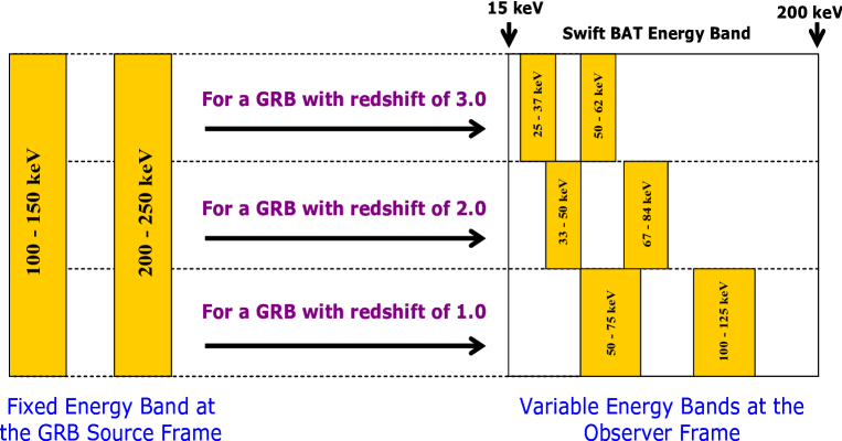
Figure 1: Fixed energy bands at the GRB source-frame are projected to various energy bands at the observer-frame, depending on the redshift.

The $Swift$ Burst Alert Telescope (BAT) is a highly sensitive instrument using a coded-mask aperture (Barthelmy et al., 2005). BAT uses the shadow pattern resulting from the coded mask to facilitate localization of the source. When a gamma-ray source illuminates the coded mask, it casts a shadow onto a position-sensitive detector. The shadow cast depends on the position of the gamma-ray source on the sky. If one knows the tile pattern in the coded mask and the geometry of the detector, it is possible to calculate the shadow patterns created by all possible points in the sky using a ray-tracing algorithm. Hence, by correlating the observed shadow, with the pre-calculated shadow, one can find the location of the source. However, each detector can be illuminated by many sources and a given source can illuminate many detectors. Hence, in order to disentangle each sky position, special algorithms have been developed and integrated in to the data analysis software by the $Swift$ BAT team.

To generate background-subtracted light curves we used a process called mask weighting. The mask weighting assigns a ray-traced shadow value for each individual event, which then enables the user to calculate light curves or spectra. We used the batmaskwtevt and batbinevt tasks in FTOOLS to generate mask weighted, background-subtracted light curves, for various observer-frame energy bands, as shown in Table 1. These are the energy bands that correspond to fixed energy bands in the source-frame i.e. $100-150$ and $200-250$ keV. These particular energy bands were selected so that after transforming to the observer-frame they lie in the detectable energy range of the $Swift$ BAT instrument (see Fig. 1). Even though the BAT can detect photons up to 350 keV, we limited the upper-boundary to 200 keV in the observer-frame. This is because the mask-weighted effective area of the detector falls rapidly after 200 keV and as a result the contribution to the light curve from energies greater than $\sim$200 keV (in observer-frame) is negligible (Sakamoto et al., 2011).

Table 1: The observer-frame energy bands and energy gaps (the energy difference between the mid-points of energy bands) for bursts in the sample.

GRB	Redshift	Low Energy Band (keV)	High Energy Band (keV)	Energy Gap (keV)
GRB050401	$2.899^{1}$	26-38	51-64	26
GRB050603	$2.821^{2}$	26-39	52-65	26
GRB050922C	$2.199^{3}$	31-47	63-78	32
GRB051111	$1.549^{4}$	39-59	78-98	39
GRB060206	$4.056^{5}$	20-30	40-49	20
GRB060210	$3.913^{6}$	20-31	41-51	21
GRB060418	$1.490^{7}$	40-60	80-100	40
GRB060904B	$0.703^{8}$	59-88	117-147	59
GRB060908	$1.884^{9}$	35-52	69-87	35
GRB060927	$5.464^{10}$	15-23	31-39	16
GRB061007	$1.262^{11}$	44-66	88-111	45
GRB061021	$0.346^{12}$	74-111	149-186	75
GRB061121	$1.315^{13}$	43-65	86-108	43
GRB070306	$1.496^{14}$	40-60	80-100	40
GRB071010B	$0.947^{15}$	51-77	103-128	52
GRB071020	$2.145^{16}$	32-48	64-79	32
GRB080319B	$0.937^{17}$	52-77	103-129	52
GRB080319C	$1.949^{18}$	34-51	68-85	34
GRB080411	$1.030^{19}$	49-74	99-123	50
GRB080413A	$2.433^{20}$	29-44	58-73	29
GRB080413B	$1.101^{21}$	48-71	95-119	48
GRB080430	$0.767^{22}$	57-85	113-141	56
GRB080603B	$2.689^{23}$	27-41	54-68	27
GRB080605	$1.640^{24}$	38-57	76-95	38
GRB080607	$3.036^{25}$	25-37	50-62	25
GRB080721	$2.591^{26}$	28-42	56-70	28
GRB080916A	$0.689^{27}$	59-89	118-148	59
GRB081222	$2.770^{28}$	27-40	53-66	26
GRB090424	$0.544^{29}$	65-97	130-162	65
GRB090618	$0.540^{30}$	65-97	130-162	65
GRB090715B	$3.000^{31}$	25-38	50-63	25
GRB090812	$2.452^{32}$	29-43	58-72	29
GRB090926B	$1.240^{33}$	45-67	89-112	45
GRB091018	$0.971^{34}$	51-76	101-127	51
GRB091020	$1.710^{35}$	37-55	74-92	37
GRB091024	$1.091^{36}$	48-72	96-120	48
GRB091029	$2.752^{37}$	27-40	53-67	27
GRB091208B	$1.063^{38}$	48-73	97-121	49
GRB100621A	$0.542^{39}$	65-97	130-162	65
GRB100814A	$1.440^{40}$	41-61	82-102	41
GRB100816A	$0.800^{41}$	56-83	111-139	56
GRB100906A	$1.727^{42}$	37-55	73-92	37
GRB110205A	$2.220^{43}$	31-47	62-78	31
GRB110213A	$1.460^{44}$	41-61	81-102	41

(1) Watson et al. (2006); (2) Berger & Becker (2005b); (3) Piranomonte et al. (2008); (4) Penprase et al. (2006); (5) Fynbo et al. (2009); (6) Fynbo et al. (2009); (7) Prochaska et al. (2006); (8) Fynbo et al. (2009); (9) Fynbo et al. (2009); (10) Fynbo et al. (2009); (11) Fynbo et al. (2009); (12) Fynbo et al. (2009); (13) Fynbo et al. (2009); (14) Jaunsen et al. (2008); (15) Cenko et al. (2007); (16) Jakobsson et al. (2007); (17) D’Elia et al. (2009); (18) Fynbo et al. (2009); (19) Fynbo et al. (2009); (20) Fynbo et al. (2009); (21) Fynbo et al. (2009); (22) Cucchiara & Fox (2008); (23) Fynbo et al. (2009); (24) Fynbo et al. (2009); (25) Prochaska et al. (2009); (26) Fynbo et al. (2009); (27) Fynbo et al. (2009); (28) Cucchiara et al. (2008); (29) Chornock et al. (2009); (30) Cenko et al. (2009); (31) Wiersema et al. (2009); (32) de Ugarte Postigo et al. (2009); (33) Fynbo et al. (2009); (34) Chen et al. (2009); (35) Xu et al. (2009); (36) Cucchiara et al. (2009); (37) Chornock et al. (2009); (38) Wiersema et al. (2009); (39) Milvang-Jensen et al. (2010); (40) O’Meara et al. (2010); (41) Tanvir et al. (2010); (42) Cenko et al. (2011); (43) Milne & Cenko (2011).

The spectral lags were extracted using the improved cross-correlation function (CCF) analysis method described in U10. In this method, the spectral lag is defined as the time delay corresponding to the global maximum of the cross-correlation function. The CCF with a delay index $d$ is defined as,

$$CCF(d,x,y)=\frac{\sum_{\small i=\textrm{max}(1,1-d)}^{\small\textrm{min}(N,N-d)}x_{i}\,y_{i+d}}{\sqrt{\sum_{i}x_{i}^{2}\,\sum_{i}y_{i}^{2}}}$$ (1)

where $x_{i}$ and $y_{i}$ are two sets of time-sequenced data spread over $N$ bins. The time delay is obtained by multiplying $d$ by the time bin size of the light curves. A Gaussian curve was fitted to the CCF (plotted as a function of time delay) to extract the spectral lag. The uncertainty in the spectral lag is obtained by simulating 1,000 light curves using the Monte Carlo technique (see U10 for more details).

The isotropic peak luminosity ($L_{\rm iso}$) and its uncertainty for each GRB is obtained using the method described in U10. In essence, a typical GRB spectrum can be described by the Band function (Band et al., 1993), for the photon flux per unit photon energy using

$$N(E)=\left\{\begin{array}[]{ll}A(\frac{E}{100\,\rm{keV}})^{\,\alpha}\,e^{-(2+\alpha)E/E_{\rm pk}},\,\small E\,\leq\,\big{(}\frac{\alpha-\beta}{2+\alpha}\big{)}E_{\rm pk}&\\ A(\frac{E}{100\,\rm{keV}})^{\,\beta}\,[\frac{(\alpha-\beta)E_{\rm pk}}{(2+\alpha)100\,\rm{keV}}]^{\alpha-\beta}\,e^{(\beta-\alpha)},\,\rm else,&\end{array}\right.$$ (2)

which has four model parameters: the amplitude (A), the low-energy spectral index ($\alpha$), the high-energy spectral index ($\beta$) and the peak ($E_{\rm pk}$) of $E^{2}N(E)$ spectrum (also called the $\nu F_{\nu}$ spectrum, apart from a factor of Planck’s constant). Using these spectral parameters the observed peak flux can be calculated for the source-frame energy-range $E_{1}=1.0\,\rm{keV}$ to $E_{2}=10,000\,\rm{keV}$ using

$$f_{\rm obs}=\int_{E_{1}/(1+z)}^{E_{2}/(1+z)}\,N(E)E\,dE.$$ (3)

The isotropic peak luminosity is defined by

$$L_{\rm iso}=4\pi d_{L}^{\,2}\,f_{\rm{obs}}$$ (4)

where $d_{L}$ is the luminosity distance:

$$d_{L}=\frac{(1+z)c}{H_{0}}\int_{0}^{z}\frac{dz^{\prime}}{\sqrt{\Omega_{M}(1+z^{\prime})^{3}+\Omega_{L}}}.$$ (5)

For the current universe we take $\Omega_{M}=0.27$, $\Omega_{L}=0.73$ and the Hubble constant $H_{0}$ to be $70\,\rm(kms^{-1})/Mpc$ (Komatsu et al., 2009). For more details of the $L_{\rm iso}$ calculation see U10.

3 Results

We employed an additional 12 long bursts to the GRB sample (31 GRBs) that was used in U10, which increased the total sample to 43. This sample has redshifts ranging from 0.346 (GRB 061021) to 5.464 (GRB 060927) with an average redshift of $\sim$2.0. The spectral information for the additional 12 bursts used in this paper is given in Table 2. The calculated peak isotropic luminosities, spanning three orders of magnitude, are given in U10 and Table 2.

Table 2: GRB redshift and spectral information. Note that uncertainties of parameters that are reported with 90% confidence level have been reduced to 1-$\sigma$ level for consistency.

GRB	Peak Flux a	$E_{\rm pk}$${}^{\,b}$	$\alpha$	$\beta^{\,c}$	$L_{\rm iso}$ erg/s	Reference
GRB090812	$3.60\pm 0.13$	$572^{+99}_{-156}$	$-1.03^{+0.04}_{-0.04}$	$-2.50^{+0.16}_{-0.16}$	$(7.86^{+1.95}_{-0.87})\times 10^{52}$	Pal’Shin et al. (2009); Baumgartner et al. (2009)
GRB090926B	$3.20\pm 0.19$	$91^{+1}_{-1}$	$-0.13^{+0.04}_{-0.04}$	$-2.36^{+0.31}_{-0.31}$	$(5.22^{+3.88}_{-0.82})\times 10^{51}$	Briggs (2009); Baumgartner et al. (2009)
GRB091018	$10.30\pm 0.25$	$28^{+10}_{-6}$	$-1.53^{+0.24}_{-0.37}$	$-2.44^{+0.15}_{-0.15}$	$(6.96^{+1.76}_{-0.58})\times 10^{51}$	Golenetskii et al. (2009); Markwardt et al. (2009)
GRB091020	$4.20\pm 0.19$	$47^{+4}_{-4}$	$-0.20^{+0.25}_{-0.25}$	$-1.70^{+0.01}_{-0.01}$	$(2.81^{+0.19}_{-0.16})\times 10^{52}$	Chaplin (2009); Palmer et al. (2009)
GRB091024	$2.00\pm 0.19$	$500^{+100}_{-100}$	$-1.10^{+0.13}_{-0.13}$	$-2.36^{+0.31}_{-0.31}$	$(5.56^{+2.43}_{-0.89})\times 10^{51}$	Golenetskii et al. (2009); Sakamoto et al. (2009)
GRB091029	$1.80\pm 0.06$	$61^{+10}_{-10}$	$-1.46^{+0.17}_{-0.17}$	$-2.36^{+0.31}_{-0.31}$	$(1.67^{+0.60}_{-0.15})\times 10^{52}$	Barthelmy et al. (2009)
GRB091208B	$15.20\pm 0.63$	$124^{+12}_{-12}$	$-1.44^{+0.04}_{-0.04}$	$-2.32^{+0.29}_{-0.12}$	$(1.68^{+0.65}_{-0.09})\times 10^{52}$	McBreen (2009); Baumgartner et al. (2009)
GRB100621A	$12.80\pm 0.19$	$95^{+8}_{-11}$	$-1.70^{+0.08}_{-0.08}$	$-2.45^{+1.44}_{-1.44}$	$(2.55^{+0.83}_{-0.34})\times 10^{51}$	Golenetskii et al. (2010); Ukwatta et al. (2010)
GRB100814A	$2.50\pm 0.13$	$106^{+7}_{-8}$	$-0.64^{+0.08}_{-0.09}$	$-2.02^{+0.08}_{-0.06}$	$(8.27^{+1.13}_{-0.69})\times 10^{51}$	von Kienlin (2010); Krimm et al. (2010)
GRB100906A	$10.10\pm 0.25$	$180^{+25}_{-28}$	$-1.10^{+0.06}_{-0.06}$	$-2.20^{+0.19}_{-0.13}$	$(4.90^{+1.23}_{-0.43})\times 10^{52}$	Golenetskii et al. (2010); Barthelmy et al. (2010)
GRB110205A	$3.60\pm 0.13$	$222^{+46}_{-46}$	$-1.52^{+0.09}_{-0.09}$	$-2.36^{+0.31}_{-0.31}$	$(2.78^{+0.57}_{-0.20})\times 10^{52}$	Golenetskii et al. (2011)
GRB110213A	$1.60\pm 0.38$	$98^{+4}_{-5}$	$-1.44^{+0.03}_{-0.03}$	$-2.36^{+0.31}_{-0.31}$	$(3.53^{+1.97}_{-0.53})\times 10^{51}$	Foley (2011); Barthelmy et al. (2011)

${}^{a}\,$ 1-second peak photon flux measured in $\rm photons\,\,cm^{-2}\,s^{-1}$ in the energy range $15-150$ keV.

${}^{b}\,$ Peak energy, $E_{\rm pk}$, is given in keV.

${}^{c}\,$ Values in brackets indicates estimated high-energy photon index, $\beta$, which is the mean value of the BATSE $\beta$ distribution (Kaneko et al., 2006; Sakamoto et al., 2009).

By choosing appropriate energy bands in the observer-frame (according to the redshift of each burst), we extracted mask-weighted background-subtracted light curves for the selected source-frame energy bands 100–150 and 200–250 keV. The observer-frame energy bands used for each burst are shown in Table 1. Note that the energy gap between the mid-point of the two source-frame energy bands is fixed at 100 keV whereas in the observer-frame, as expected, this gap varies depending on the redshift of each burst (see the Table 1). For example, in GRB 060927, this gap is 16 keV and in GRB 061021, it is 75 keV. This is in contrast to the spectral lag extractions performed in the observer-frame where this gap is treated as a constant.

The extracted spectral lags for the source-frame energy bands 100–150 and 200–250 keV are listed in Table 3. The $Swift$ BAT trigger ID, the segment of the light curve used for the lag extraction ($T+X_{\rm S}$ and $T+X_{\rm E}$, $T$ is the trigger time), the time binning of the light curve, and the Gaussian curve fitting range of the CCF vs time delay plot (with start time, and end time denoted as $LS$ and $LE$ respectively) are also given in Table 3. Of 43 bursts in the sample there are 24 bursts which have lags greater than zero. The remaining 19 bursts either have lags consistent with zero (16 bursts) or negative values (3 bursts).

For the 24 bursts which have positive lags with significance 1-$\sigma$ or greater (see Table 3), we find that the redshift corrected lag is anti-correlated with $L_{\rm iso}$. The correlation coefficient for this relation is -0.82 $\pm$ 0.05 with a chance probability of $\sim 5.54\times 10^{-5}$. The extracted correlation coefficient is significantly higher than the correlation coefficient (averaged over the six combinations of standard BAT energy channels) of $\sim\,-0.68$ reported in U10. Various correlation coefficients of the relation are shown in Table 4, where uncertainties in the correlation coefficients were obtained through a Monte Carlo simulation utilizing uncertainties in $L_{\rm iso}$ and the lag values. The null probability that the correlation occurs due to random chance is also given for each coefficient type.

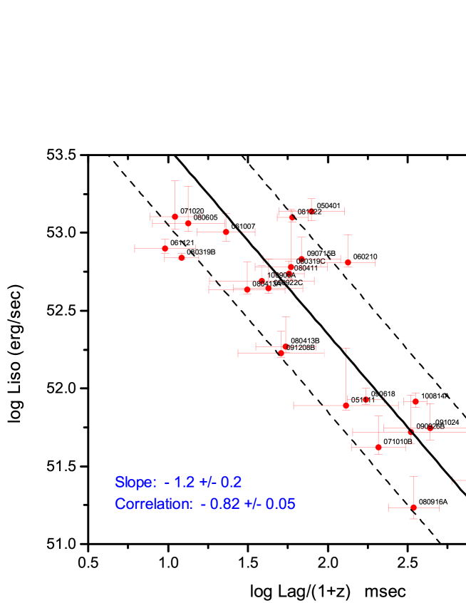
Figure 2: The spectral lags between the source-frame energy range bands $100-150$ keV and $200-250$ keV and the isotropic peak luminosity are plotted in a log-log plot.

Fig. 2 shows a log-log plot of isotropic peak luminosity vs redshift-corrected spectral lag. The solid line shows the following best-fit power-law curve:

$$\log\bigg{(}\frac{L_{\rm iso}}{{\rm erg/s}}\bigg{)}=(54.7\pm 0.4)-(1.2\pm 0.2)\log\frac{Lag/({\rm ms})}{1+z}.$$ (6)

Since there is considerable scatter, the uncertainties of the fit parameters are multiplied by a factor of $\sqrt{\rm\chi^{2}/ndf}=\sqrt{84.36/22}=1.96$. The dash lines indicate the estimated 1-$\sigma$ confidence level, which is obtained from the cumulative fraction of the residual distribution taken from 16% to 84%.

The best-fit power-law index ($-1.2\pm 0.2$) is consistent with observer-frame results obtained by Norris et al. (2000) ($\sim\,-1.14$) and the average power-law index of $-1.4\pm 0.3$ reported in U10.

Table 3: Source-frame spectral lag values of long duration $Swift$ BAT GRBs

GRB	Trigger ID	$T+X_{\rm S}$ (s)	$T+X_{\rm E}$ (s)	Bin Size (ms)	LS (s)	LE (s)	Lag Value (ms)	Significance
GRB050401	113120	23.03	29.43	64	-2.00	2.00	310$\pm$145	2.14
GRB050603	131560	-3.83	3.08	16	-0.40	0.40	-16$\pm$21	-0.76
GRB050922C	156467	-2.70	2.94	16	-1.00	1.00	136$\pm$68	2.00
GRB051111	163438	-6.96	28.62	64	-4.00	4.00	333$\pm$251	1.33
GRB060206	180455	-1.29	8.18	16	-2.00	2.00	86$\pm$111	0.77
GRB060210	180977	-3.37	5.08	128	-4.00	4.00	658$\pm$259	2.54
GRB060418	205851	-7.66	33.04	64	-2.00	2.00	-110$\pm$106	-1.04
GRB060904B	228006	-1.97	10.32	512	-6.00	6.00	124$\pm$436	0.28
GRB060908	228581	-10.91	3.68	32	-2.00	2.00	78$\pm$124	0.63
GRB060927	231362	-1.69	8.04	32	-1.00	1.00	18$\pm$75	0.24
GRB061007	232683	23.86	65.08	4	-0.20	0.20	52$\pm$22	2.36
GRB061021	234905	-0.46	14.64	512	-4.00	4.00	-430$\pm$975	-0.44
GRB061121	239899	60.44	80.66	4	-0.20	0.20	22$\pm$10	2.20
GRB070306	263361	90.00	118.42	32	-4.00	2.00	-362$\pm$247	-1.47
GRB071010B	293795	-1.70	17.24	64	-2.00	2.00	404$\pm$159	2.54
GRB071020	294835	-3.22	1.14	4	-0.20	0.40	35$\pm$13	2.69
GRB080319B	306757	-2.85	57.57	4	-0.10	0.14	23$\pm$6	3.83
GRB080319C	306778	-0.77	13.31	32	-1.00	1.00	174$\pm$91	1.91
GRB080411	309010	38.46	48.45	4	-0.50	0.50	116$\pm$25	4.64
GRB080413A	309096	-0.42	9.05	8	-1.00	1.00	107$\pm$59	1.81
GRB080413B	309111	-1.44	4.96	32	-1.00	1.00	115$\pm$50	2.30
GRB080430	310613	-1.24	12.84	256	-4.00	4.00	91$\pm$431	0.21
GRB080603B	313087	-0.54	5.10	16	-1.00	1.00	5$\pm$59	0.08
GRB080605	313299	-5.46	15.53	8	-0.20	0.20	35$\pm$18	1.94
GRB080607	313417	-6.13	12.05	8	-0.50	0.50	26$\pm$30	0.87
GRB080721	317508	-3.39	8.64	64	-2.00	2.00	-86$\pm$110	-0.78
GRB080916A	324895	-2.66	39.58	128	-2.00	4.00	585$\pm$214	2.73
GRB081222	337914	-0.80	15.58	4	-1.00	1.00	227$\pm$51	4.45
GRB090424	350311	-0.94	4.95	16	-0.20	0.20	14$\pm$14	1.00
GRB090618	355083	46.01	135.35	8	-2.00	2.00	267$\pm$72	3.71
GRB090715B	357512	-4.80	21.06	16	-2.00	3.00	275$\pm$155	1.77
GRB090812	359711	-6.93	41.20	256	-6.00	6.00	-22$\pm$202	-0.11
GRB090926B	370791	-22.00	36.00	512	-10.00	8.00	746$\pm$627	1.19
GRB091018	373172	-0.28	2.92	64	-2.00	1.00	143$\pm$297	0.48
GRB091020	373458	-2.54	13.84	128	-3.00	2.00	-187$\pm$177	-1.06
GRB091024	373674	-9.58	27.29	512	-10.00	10.00	912$\pm$604	1.51
GRB091029	374210	-4.03	38.98	256	-10.00	10.00	-112$\pm$395	-0.28
GRB091208B	378559	7.66	10.61	64	-1.00	1.00	105$\pm$66	1.59
GRB100621A	425151	-6.79	40.31	256	-3.00	3.00	1199$\pm$311	3.86
GRB100814A	431605	-4.40	29.39	256	-4.00	4.00	862$\pm$147	5.86
GRB100906A	433509	-1.49	26.16	128	-2.00	2.00	105$\pm$79	1.33
GRB110205A	444643	118.89	293.99	64	-1.00	1.00	-29$\pm$52	-0.56
GRB110213A	445414	-3.42	5.29	512	-3.00	3.50	602$\pm$746	0.81

Table 4: Correlation coefficients of the lag–luminosity relation.

Coefficient Type	Correlation Coefficient	Null Probability
Pearson’s $r$	- 0.82$\pm$0.05	$5.54\,\times\,10^{-5}$
Spearman’s $r_{\rm s}$	- 0.70$\pm$0.06	$1.49\,\times\,10^{-4}$
Kendall’s $\tau$	- 0.50$\pm$0.05	$6.63\,\times\,10^{-4}$

4 Discussion

4.1 Spectral Lags: Observer-frame versus Source-frame

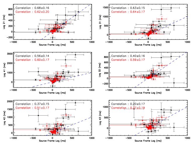
Figure 3: All combinations of fixed observer-frame energy channel (canonical BAT energy bands: channel 1 (15–25 keV), 2 (25–50 keV), 3 (50–100 keV) and 4 (100–200 keV)) spectral lag values as a function of fixed source-frame energy channel (between 100–150 keV and 200–250 keV) lag values. Black and red data points and labels corresponds to redshift uncorrected and corrected cases respectively. The blue dashed line corresponds to the equality line of the two parameters in each panel.

U10 extracted spectral lags in fixed energy bands in the observer-frame and in this work for the same sample of 31 bursts we extracted lags in fixed energy bands in the source-frame. In the observer-frame case, there are four energy channels (canonical BAT energy bands: channel 1 (15–25 keV), 2 (25–50 keV), 3 (50–100 keV) and 4 (100–200 keV)), thus six lag extractions per burst. It is interesting to study to what degree these different lags correlate with source-frame lags (between fixed source-frame energy channels 100–150 keV and 200–250 keV). In Fig. 3 we show all combinations of observer-frame lags as a function of source-frame lags. The red data points show lags with the time-dilation correction due to cosmological redshift and black data points show lags without the time-dilation correction. From Fig. 3 it is clear that all plots show some correlation both in the time-dilation corrected (shown in red) and time-dilation uncorrected (shown in black) cases. We note that the correlation coefficients are greater than 0.5 in time-dilation uncorrected cases where BAT channel 1 is involved in the lag extraction. In the time-dilation corrected case all plots show correlation coefficients greater than 0.5 except for the Lag43 plot. Despite these moderate correlation coefficients, the large scatter seen in these plots indicate that the observer-frame lag does not directly represent the source-frame lag.

4.2 Lag-$L_{\rm iso}$ Relation: Observer-frame versus Source-frame

There are two important changes in the Lag-Luminosity relation which may occur when going from fixed observer-frame energy bands to fixed source-frame energy bands: A change in the power-law index, and a change in the dispersion of the data measured by the correlation coefficient. Table 5 summarizes these two parameters for various energy bands both in the observer-frame and in the source-frame.

In the observer-frame the power-law index varies from $\sim 0.6$ to $\sim 1.8$, with mean around 1.3. In the source-frame the index changes from 0.9 to 1.23 with a mean of $\sim$1.1. Meanwhile, the correlation coefficient varies from 0.60 to 0.79 in the observer-frame and in the source-frame it changes from 0.76 to 0.90. Hence, according to Table 5, the source-frame Lag-$L_{\rm iso}$ relation seems to be tighter than the observer-frame case with a slope closer to one.

Table 5: Observer-frame and source-frame slopes and correlation coefficients of the lag-$L_{\rm iso}$ relation. Conservative 10% uncertainty is assumed for cases without uncertainties.

Energy Bands	Frame	Slope	Correlation Coefficient	Number of GRBs	Reference
(0.3-1), (3-10) keV	Observer	0.95$\pm$0.23	-	9	Margutti et al. (2010)
(6-25), (50-400) keV	Observer	1.16$\pm$0.07	- 0.79${}^{+0.16}_{-0.05}$	8	Arimoto et al. (2010)
(15-25), (25-50) keV	Observer	1.4$\pm$0.1	- 0.63$\pm$0.06	21	U10
(15-25), (50-100) keV	Observer	1.5$\pm$0.1	- 0.60$\pm$0.06	28	U10
(15-25), (100-200) keV	Observer	1.8$\pm$0.1	- 0.67$\pm$0.07	27	U10
(25-50), (50-100) keV	Observer	1.2$\pm$0.1	- 0.66$\pm$0.07	27	U10
(25-50), (100-200) keV	Observer	1.4$\pm$0.1	- 0.75$\pm$0.07	25	U10
(25-50), (100-300) keV	Observer	1.14$\pm$0.1	-	6	Norris et al. (2000)
(25-50), (100-300) keV	Observer	0.62$\pm$0.04	-0.72$\pm$0.07	6	Hakkila et al. (2008)
(50-100), (100-200) keV	Observer	1.4$\pm$0.1	- 0.77$\pm$0.08	22	U10
(20-100), (100-500) keV	Source	1.23$\pm$0.07	- 0.90${}^{+0.12}_{-0.02}$	8	Arimoto et al. (2010)
(100-200), (300-400) keV	Source	0.9$\pm$0.1	- 0.76$\pm$0.06	22	Ukwatta et al. (2010b)
(100-150), (200-250) keV	Source	1.2$\pm$0.2	- 0.82$\pm$0.05	24	This work

4.3 Spectral Lag - $E_{\rm pk}$ Relation

Now we investigate the relation between source-frame spectral lag and source-frame average peak energy ($E_{\rm pk}(1+z)$) of the burst spectrum. In Fig. 4, we plotted $E_{\rm pk}(1+z)$ as a function of source-frame lags. There is a correlation between these two parameters with a correlation coefficient of $-0.57\pm 0.14$. Various correlation coefficients of the relation are shown in Table 6, with uncertainties and null probabilities.

The best-fit is shown as a dashed line in Fig. 4, yielding the following relation between $E_{\rm pk}(1+z)$ and $Lag/(1+z)$:

$$\log\bigg{(}\frac{E_{\rm pk}(1+z)}{\rm keV}\bigg{)}=(3.7\pm 0.1)-(0.56\pm 0.06)\log\frac{Lag/({\rm ms})}{1+z}.$$ (7)

The uncertainties in the fitted parameters are expressed with the factor of $\sqrt{\rm\chi^{2}/ndf}=\sqrt{30.71/22}\approx 1.18$.

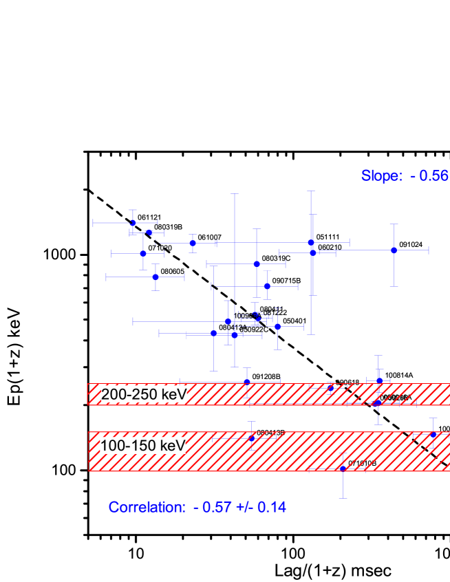
Figure 4: The source-frame peak energy ($E_{\rm pk}(1+z)$) versus source-frame spectral lags. The energy bands, $100-150$ keV and $200-250$ keV, corresponding to the lag extractions are shown in hashed red bands on the plot.

According to equation (6), $L_{\rm iso}\propto(Lag/(1+z))^{-1.2}$. From the Yonetoku relation we know that $L_{\rm iso}\propto(E_{\rm pk}(1+z))^{2.0}$ (Yonetoku et al., 2004). Hence, from these two relations we expect to see a correlation between $E_{\rm pk}(1+z)$ and $Lag/(1+z)$ such as $E_{\rm pk}(1+z)\propto(Lag/(1+z))^{-0.6}$.

The best fit slope of $0.56\pm 0.06$ is consistent with the expected slope of $\sim$ 0.6 based on the source-frame lag-luminosity and the Yonetoku relation. However, note that the correlation coefficient is significantly smaller than the coefficient for the lag-luminosity relation. This lower degree of correlation may be suggestive of brightness and detector related selection effects that have been noted in the literature (Butler et al., 2007) for the Yonetoku relation.

Table 6: Correlation coefficients of the lag–$E_{\rm pk}$ relation.

Coefficient Type	Correlation Coefficient	Null Probability
Pearson’s $r$	- 0.57$\pm$0.14	$4.83\,\times\,10^{-3}$
Spearman’s $r_{\rm s}$	- 0.50$\pm$0.12	$1.36\,\times\,10^{-2}$
Kendall’s $\tau$	- 0.37$\pm$0.14	$1.18\,\times\,10^{-2}$

4.4 Some Models for Spectral Lags

U10 and this work have provided more evidence for the existence of the lag-luminosity relation based on a sample of $Swift$ BAT GRBs with measured spectroscopic redshifts. This analysis calls for a physical interpretation for spectral lag and a lag-luminosity relation. In the literature, several possible interpretations have been discussed (Dermer, 1998; Salmonson, 2000; Ioka & Nakamura, 2001; Kocevski & Liang, 2003; Schaefer, 2004; Qin et al., 2004; Ryde, 2005; Shen et al., 2005; Lu et al., 2006; Peng et al., 2011).

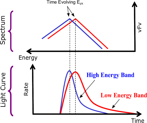
Figure 5: The time evolution of the $E_{\rm pk}$ across energy bands may cause the observed spectral lags in GRBs.

One proposed explanation for the observed spectral lag is the spectral evolution during the prompt phase of the GRB (Dermer, 1998; Kocevski & Liang, 2003; Ryde, 2005). Due to cooling effects, $E_{\rm pk}$ moves to a lower energy channel after some characteristic time. When the peak energy ($E_{\rm pk}$) moves from a higher energy band to a lower energy band, the temporal peak of the light curve also moves from a higher energy band to a lower one, which results in the observed spectral lag. In a recent study, Peng et al. (2011) suggest that spectral evolution can be invoked to explain both positive and negative spectral lags. Hard-to-soft evolution of the spectrum produces positive spectral lags while soft-to-hard evolution would lead to negative lags. In addition, these authors also suggest that soft-to-hard-to-soft evolution may produce negative lags.

A schematic diagram showing a hard-to-soft scenario is depicted in Fig. 5. Initially, $E_{\rm pk}$ of the spectrum is in the high-energy band, which results in a pulse in the light curve of the high energy band. Then $E_{\rm pk}$ moves to the lower energy band resulting in a pulse in the low-energy light curve. The temporal difference between the two pulses in the light curves would then be a measure of the cooling time scale of the spectrum.

If this were the only process that caused the lag then in a simple picture one would expect the source-frame average $E_{\rm pk}$ to lie within the two energy bands in question. According to Fig. 4, for the majority of bursts the source-frame $E_{\rm pk}$ lies outside the energy band $100-250$ keV, indicating that the simple spectral evolution scenario described above may not be the dominant process responsible for the observed lags. However, it is worth noting that a pulse in a specific energy band may not always mean that the $E_{\rm pk}$ is also within that energy band. There are other issues associated with this model: 1) the calculated cooling times based on simple synchrotron models are, in general, relatively small compared to the extracted lags, and 2) short bursts which exhibit considerable spectral evolution do not show significant lags.

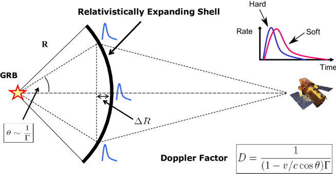
Figure 6: Spectral lags could arise due to the curvature effect of the shocked shell. At the source, the relativistically expanding shell emits identical pulses from all latitudes. However, when the photons reach the detector, on-axis photons get boosted to higher energy (hard). Meanwhile off-axis photons get relatively smaller boost and travel longer to reach the detector. Thus these photons are softer and arrive later than the on-axis photons.

Another model that purports to explain spectral lags is based on the curvature effect, i.e., a kinematics effect due to the observer looking at increasingly off-axis annulus areas relative to the line-of-sight (Salmonson, 2000; Ioka & Nakamura, 2001; Dermer, 2004; Shen et al., 2005; Lu et al., 2006). Fig. 6 illustrates how the spectral lag could arise due to the curvature effect of the shocked shell. Due to a smaller Doppler factor and a path difference, the radiation from shell areas which are further off axis will be softer and therefore lead to a lag. As with spectral evolution models, there are difficulties associated with the curvature models too. These kinematic models generally predict only positive lags. As can be seen from Table 3 some of the measured lags are negative, and therefore these lags present a real challenge for the simple curvature models.

It is possible that spectral lags are caused by multiple mechanisms. Peng et al. (2011) investigated spectral lags caused by intrinsic spectral evolution and the curvature effect combined. They showed that the curvature effect always tends to increase the observed spectral lag in the positive direction. Even for cases with soft-to-hard spectral evolution, when the curvature effect is introduced lags become positive. Hence they predict that the majority of measured spectral lags should be positive, which is consistent with the findings of this work and U10.

5 Summary and Conclusion

We have investigated the spectral lag between $100-150$ keV and $200-250$ keV energy bands at the GRB source-frame by projecting these bands to the observer-frame. This is a step forward in the investigation of lag-luminosity relations since most of the previous investigations used arbitrary observer-frame energy bands.

Our analysis has produced an improved correlation between spectral lag ($\tau$) and isotropic luminosity over those previously reported with the following relation:

$$\frac{\tau/(\rm ms)}{1+z}\cong\bigg{[}\frac{L_{\rm iso}/(\rm erg\,s^{-1})}{10^{54.7}}\bigg{]}^{-0.8}.$$ (8)

We also find a modest correlation between the source-frame spectral lag and the peak energy of the burst, which is given by the relation,

$$\frac{\tau/(\rm ms)}{1+z}\cong\bigg{[}\frac{E_{\rm pk}(1+z)/(\rm keV)}{10^{3.7}}\bigg{]}^{-1.8}.$$ (9)

Finally, we mentioned two simple models and noted their limitations in explaining the observed spectral lags.

References

- Arimoto et al. (2010) Arimoto, M., et al. 2010, PASJ, 62, 487
- Band (1997) Band, D. L. 1997, ApJ., 486, 928
- Band et al. (1993) Band, D., et al. 1993, ApJ., 413, 281
- Barthelmy et al. (2005) Barthelmy, S. D., et al. 2005a, Space Sci. Rev., 120, 143
- Barthelmy et al. (2009) Barthelmy, S. D., et al. 2009, GRB Coordinates Network, Circular Service, 10103, 1
- Barthelmy et al. (2010) Barthelmy, S. D., et al. 2010, GRB Coordinates Network, Circular Service, 11233, 1
- Barthelmy et al. (2011) Barthelmy, S. D., et al. 2011, GRB Coordinates Network, Circular Service, 11714, 1
- Baumgartner et al. (2009) Baumgartner, W. H., et al. 2009, GRB Coordinates Network, Circular Service, 10265, 1
- Baumgartner et al. (2009) Baumgartner, W. H., et al. 2009, GRB Coordinates Network, 9775, 1
- Baumgartner et al. (2009) Baumgartner, W. H., et al. 2009, GRB Coordinates Network, 9939, 1
- Berger & Becker (2005b) Berger, E., & Becker, G. 2005, GRB Coordinates Network, 3520, 1
- Briggs (2009) Briggs, M. S. 2009, GRB Coordinates Network, 9957, 1
- Butler et al. (2007) Butler, N. R., Kocevski, D., Bloom, J. S., & Curtis, J. L. 2007, ApJ., 671, 656
- Cenko et al. (2007) Cenko, S. B., Cucchiara, A., Fox, D. B., Berger, E., & Price, P. A. 2007, GRB Coordinates Network, 6888, 1
- Cenko et al. (2009) Cenko, S. B., et al. 2009, GRB Coordinates Network, 9518, 1
- Cenko et al. (2011) Cenko, S. B., Hora, J. L., & Bloom, J. S. 2011, GRB Coordinates Network, Circular Service, 11638, 1
- Chaplin (2009) Chaplin, V. 2009, GRB Coordinates Network, Circular Service, 10095, 1
- Chen et al. (2009) Chen, H.-W., Helsby, J., Shectman, S., Thompson, I., & Crane, J. 2009, GRB Coordinates Network, Circular Service, 10038, 1
- Chornock et al. (2009) Chornock, R., Perley, D. A., Cenko, S. B., & Bloom, J. S. 2009, GRB Coordinates Network, 9243, 1
- Chornock et al. (2009) Chornock, R., Perley, D. A., & Cobb, B. E. 2009, GRB Coordinates Network, Circular Service, 10100, 1
- Cucchiara & Fox (2008) Cucchiara, A., & Fox, D. B. 2008, GRB Coordinates Network, 7654, 1
- Cucchiara et al. (2006) Cucchiara, A., Fox, D. B., & Berger, E. 2006, GRB Coordinates Network, 4729, 1
- Cucchiara et al. (2008) Cucchiara, A., Fox, D. B., Cenko, S. B., & Berger, E. 2008, GRB Coordinates Network, 8713, 1
- Cucchiara et al. (2009) Cucchiara, A., Fox, D., & Tanvir, N. 2009, GRB Coordinates Network, Circular Service, 10065, 1
- D’Elia et al. (2009) D’Elia, V., et al. 2009, ApJ., 694, 332
- Dermer (1998) Dermer, C. D. 1998, ApJ. Lett., 501, L157
- Dermer (2004) Dermer, C. D. 2004, ApJ., 614, 284
- Dermer & Menon (2009) Dermer, C. D., & Menon, G. 2009, High Energy Radiation from Black Holes: Gamma Rays, Cosmic Rays, and Neutrinos by Charles D. Dermer and Govind Menon. Princeton Univerisity Press, November 2009
- Fenimore et al. (1995) Fenimore, E. E., in ’t Zand, J. J. M., Norris, J. P., Bonnell, J. T., & Nemiroff, R. J. 1995, ApJ. Lett., 448, L101
- Foley (2011) Foley, S. 2011, GRB Coordinates Network, Circular Service, 11727, 1
- Fynbo et al. (2006) Fynbo, J. P. U., Limousin, M., Castro Cerón, J. M., Jensen, B. L., & Naranen, J. 2006, GRB Coordinates Network, 4692, 1
- Fynbo et al. (2009) Fynbo, J. P. U., Malesani, D., Jakobsson, P., & D’Elia, V. 2009, GRB Coordinates Network, 9947, 1
- Fynbo et al. (2009) Fynbo, J. P. U., et al. 2009, arXiv:0907.3449
- Gehrels et al. (2004) Gehrels, N., et al. 2004, ApJ., 611, 1005
- Gehrels et al. (2006) Gehrels, N., et al. 2006, Nature, 444, 1044
- Golenetskii et al. (2009) Golenetskii, S., Aptekar, R., Mazets, E., Pal’Shin, V., Frederiks, D., Oleynik, P., Ulanov, M., & Svinkin, D. 2009, GRB Coordinates Network, Circular Service, 10045, 1
- Golenetskii et al. (2009) Golenetskii, S., et al. 2009, GRB Coordinates Network, Circular Service, 10083, 1
- Golenetskii et al. (2010) Golenetskii, S., et al. 2010, GRB Coordinates Network, Circular Service, 10882, 1
- Golenetskii et al. (2010) Golenetskii, S., et al. 2010, GRB Coordinates Network, Circular Service, 11251, 1
- Golenetskii et al. (2011) Golenetskii, S., et al. 2011, GRB Coordinates Network, Circular Service, 11659, 1
- Hakkila et al. (2008) Hakkila, J., Giblin, T. W., Norris, J. P., Fragile, P. C., & Bonnell, J. T. 2008, ApJ. Lett., 677, L81
- Ioka & Nakamura (2001) Ioka, K., & Nakamura, T. 2001, ApJ. Lett., 554, L163
- Jakobsson et al. (2005) Jakobsson, P., Fynbo, J. P. U., Paraficz, D., Telting, J., Jensen, B. L., Hjorth, J., & Castro Cerón, J. M. 2005, GRB Coordinates Network, 4029, 1
- Jakobsson et al. (2007) Jakobsson, P., Vreeswijk, P. M., Hjorth, J., Malesani, D., Fynbo, J. P. U., & Thoene, C. C. 2007, GRB Coordinates Network, 6952, 1
- Jakobsson et al. (2008b) Jakobsson, P., Vreeswijk, P. M., Xu, D., & Thoene, C. C. 2008, GRB Coordinates Network, 7832, 1
- Jaunsen et al. (2008) Jaunsen, A. O., et al. 2008, ApJ., 681, 453
- Kaneko et al. (2006) Kaneko, Y., Preece, R. D., Briggs, M. S., Paciesas, W. S., Meegan, C. A., & Band, D. L. 2006, ApJS, 166, 298
- Kocevski & Liang (2003) Kocevski, D., & Liang, E. 2003, ApJ., 594, 385
- Komatsu et al. (2009) Komatsu, E., et al. 2009, ApJS, 180, 330
- Kouveliotou et al. (1993) Kouveliotou, C., Meegan, C. A., Fishman, G. J., Bhat, N. P., Briggs, M. S., Koshut, T. M., Paciesas, W. S., & Pendleton, G. N. 1993, ApJ. Lett., 413, L101
- Krimm et al. (2010) Krimm, H. A., et al. 2010, GRB Coordinates Network, Circular Service, 11094, 1
- Lu et al. (2006) Lu, R.-J., Qin, Y.-P., Zhang, Z.-B., & Yi, T.-F. 2006, MNRAS, 367, 275
- Margutti et al. (2010) Margutti, R., Guidorzi, C., Chincarini, G., Bernardini, M. G., Genet, F., Mao, J., & Pasotti, F. 2010, MNRAS, 406, 2149
- Markwardt et al. (2009) Markwardt, C. B., et al. 2009, GRB Coordinates Network, Circular Service, 10040, 1
- McBreen (2009) McBreen, S. 2009, GRB Coordinates Network, Circular Service, 10266, 1
- Milne & Cenko (2011) Milne, P. A., & Cenko, S. B. 2011, GRB Coordinates Network, Circular Service, 11708, 1
- Milvang-Jensen et al. (2010) Milvang-Jensen, B., et al. 2010, GRB Coordinates Network, Circular Service, 10876, 1
- Mosquera Cuesta et al. (2008) Mosquera Cuesta, H. J., Turcati, R., Furlanetto, C., Khachatryan, H. G., Mirzoyan, S., & Yegorian, G. 2008, A.& A., 487, 47
- Murakami et al. (2003) Murakami, T., Yonetoku, D., Izawa, H., & Ioka, K. 2003, PASJ, 55, L65
- Norris (1995) Norris, J. P. 1995, Ap&SS, 231, 95
- Norris (2002) Norris, J. P. 2002, ApJ., 579, 386
- Norris & Bonnell (2006) Norris, J. P., & Bonnell, J. T. 2006, ApJ., 643, 266
- Norris et al. (2000) Norris, J. P., Marani, G. F., & Bonnell, J. T. 2000, ApJ., 534, 248
- Norris et al. (1996) Norris, J. P., Nemiroff, R. J., Bonnell, J. T., Scargle, J. D., Kouveliotou, C., Paciesas, W. S., Meegan, C. A., & Fishman, G. J. 1996, ApJ., 459, 393
- Norris et al. (2005) Norris, J. P., Bonnell, J. T., Kazanas, D., Scargle, J. D., Hakkila, J., & Giblin, T. W. 2005, ApJ., 627, 324
- O’Meara et al. (2010) O’Meara, J., Chen, H.-W., & Prochaska, J. X. 2010, GRB Coordinates Network, Circular Service, 11089, 1
- Pal’Shin et al. (2009) Pal’Shin, V., et al. 2009, GRB Coordinates Network, 9821, 1
- Palmer et al. (2009) Palmer, D. M., et al. 2009, GRB Coordinates Network, Circular Service, 10051, 1
- Peng et al. (2011) Peng, Z. Y., Yin, Y., Bi, X. W., Bao, Y. Y., & Ma, L. 2011, Astronomische Nachrichten, 332, 92
- Penprase et al. (2006) Penprase, B. E., et al. 2006, ApJ., 646, 358
- Piranomonte et al. (2008) Piranomonte, S., et al. 2008, A.& A., 492, 775
- Prochaska et al. (2006) Prochaska, J. X., Chen, H.-W., Bloom, J. S., Falco, E., & Dupree, A. K. 2006, GRB Coordinates Network, 5002, 1
- Prochaska et al. (2008) Prochaska, J. X., Shiode, J., Bloom, J. S., Perley, D. A., Miller, A. A., Starr, D., Kennedy, R., & Brewer, J. 2008, GRB Coordinates Network, 7849, 1
- Prochaska et al. (2009) Prochaska, J. X., et al. 2009, ApJ. Lett., 691, L27
- Qin et al. (2004) Qin, Y.-P., Zhang, Z.-B., Zhang, F.-W., & Cui, X.-H. 2004, ApJ., 617, 439
- Rol et al. (2006) Rol, E., Jakobsson, P., Tanvir, N., & Levan, A. 2006, GRB Coordinates Network, 5555, 1
- Ryde (2005) Ryde, F. 2005, A.& A., 429, 869
- Sakamoto et al. (2008) Sakamoto, T., et al. 2008, ApJS, 175, 179
- Sakamoto et al. (2009) Sakamoto, T., et al. 2009, GRB Coordinates Network, Circular Service, 10072, 1
- Sakamoto et al. (2009) Sakamoto, T., et al. 2009, GRB Coordinates Network, 9231, 1
- Sakamoto et al. (2009) Sakamoto, T., et al. 2009, ApJ., 693, 922
- Sakamoto et al. (2011) Sakamoto, T., et al. 2011, arXiv:1104.4689
- Salmonson (2000) Salmonson, J. D. 2000, ApJ. Lett., 544, L115
- Salmonson & Galama (2002) Salmonson, J. D., & Galama, T. J. 2002, ApJ., 569, 682
- Sato et al. (2008) Sato, G., et al. 2008, GRB Coordinates Network, 7591, 1
- Sbarufatti et al. (2008) Sbarufatti, B., et al. 2008, GCN Report, 142, 1
- Schady et al. (2009) Schady, P., Baumgartner, W. H., & Beardmore, A. P. 2009, GCN Report, 232, 1
- Schaefer (2004) Schaefer, B. E. 2004, ApJ., 602, 306
- Schaefer (2007) Schaefer, B. E. 2007, ApJ., 660, 16
- Shen et al. (2005) Shen, R.-F., Song, L.-M., & Li, Z. 2005, MNRAS, 362, 59
- Stamatikos et al. (2009) Stamatikos, M., et al. 2009, American Institute of Physics Conference Series, 1133, 356
- Tanvir et al. (2010) Tanvir, N. R., Wiersema, K., & Levan, A. J. 2010, GRB Coordinates Network, Circular Service, 11230, 1
- Ukwatta et al. (2010) Ukwatta, T. N., et al. 2010, GCN Report, 291, 1
- Ukwatta et al. (2010a) Ukwatta, T. N., et al. 2010a, ApJ., 711, 1073 (U10)
- Ukwatta et al. (2010b) Ukwatta, T. N., Dhuga, K. S., Stamatikos, M., Sakamoto, T., Parke, W. C., Barthelmy, S. D., & Gehrels, N. 2010b, arXiv:1003.0229
- Watson et al. (2006) Watson, D., et al. 2006, ApJ., 652, 1011
- Wiersema et al. (2009) Wiersema, K., et al. 2009, GRB Coordinates Network, 9673, 1
- Wiersema et al. (2009) Wiersema, K., Tanvir, N. R., Cucchiara, A., Levan, A. J., & Fox, D. 2009, GRB Coordinates Network, Circular Service, 10263, 1
- Xu et al. (2009) Xu, D., et al. 2009, GRB Coordinates Network, Circular Service, 10053, 1
- Yonetoku et al. (2004) Yonetoku, D., Murakami, T., Nakamura, T., Yamazaki, R., Inoue, A. K., & Ioka, K. 2004, ApJ., 609, 935
- Zhang et al. (2006) Zhang, Z., Xie, G. Z., Deng, J. G., & Jin, W. 2006, MNRAS, 373, 729
- Zhang et al. (2009) Zhang, B., et al. 2009, ApJ., 703, 1696
- de Ugarte Postigo et al. (2009) de Ugarte Postigo, A., Gorosabel, J., Fynbo, J. P. U., Wiersema, K., & Tanvir, N. 2009, GRB Coordinates Network, 9771, 1
- von Kienlin (2010) von Kienlin, A. 2010, GRB Coordinates Network, Circular Service, 11099, 1