Geometric Exponents
of Dilute Logarithmic Minimal Models

Abstract

The fractal dimensions of the hull, the external perimeter and of the red bonds are measured through Monte Carlo simulations for dilute minimal models, and compared with predictions from conformal field theory and SLE methods. The dilute models used are those first introduced by Nienhuis. Their loop fugacity is $\beta=-2\cos(\pi/\bar{\kappa})$ where the parameter $\bar{\kappa}$ is linked to their description through conformal loop ensembles. It is also linked to conformal field theories through their central charges $c(\bar{\kappa})=13-6(\bar{\kappa}+\bar{\kappa}^{-1})$ and, for the minimal models of interest here, $\bar{\kappa}=p/p^{\prime}$ where $p$ and $p^{\prime}$ are two coprime integers. The geometric exponents of the hull and external perimeter are studied for the pairs $(p,p^{\prime})=(1,1),(2,3),(3,4),(4,5),(5,6),(5,7)$, and that of the red bonds for $(p,p^{\prime})=(3,4)$. Monte Carlo upgrades are proposed for these models as well as several techniques to improve their speeds. The measured fractal dimensions are obtained by extrapolation on the lattice size $H,V\rightarrow\infty$. The extrapolating curves have large slopes; despite these, the measured dimensions coincide with theoretical predictions up to three or four digits. In some cases, the theoretical values lie slightly outside the confidence intervals; explanations of these small discrepancies are proposed.
Keywords: dilute logarithmic minimal models; logarithmic minimal models; conformal field theory; conformal loop ensembles; SLE; fractal dimensions; geometric exponents; Monte Carlo simulations.

1 Introduction

Geometric objects remain a central tool in the study of the critical behavior of statistical lattice models. Some of the most natural ones are the hull of a spin cluster, its mass, external perimeter and red bonds. Even though they were investigated as early as in the 1970’s, their role has remained central over the years. In the 1980’s, their close ties to conformal weights of the Virasoro algebra, and more generally with conformal field theory (CFT), was revealed starting with works by Saleur and Duplantier [24]. And in the late 1990’s, techniques from probability theory related their properties to that of random curves grown through stochastic Loewner evolution (SLE). The goal of this paper is to measure, using Monte Carlo simulations, the fractal dimensions of these objects for dilute lattice models.

Recently, Saint-Aubin et al. [23] measured these dimensions for a family of lattice loop models whose continuum scaling limit is called the logarithmic minimal models (Pearce et al. [20]). Their results gave compelling evidence for the theoretical predictions of Saleur and Duplantier [24] and others, and confirmed the rigorous result by Beffara [4] for the hull fractal dimension. Their work probed the dense phase of loop models and the present paper can be seen as completing their work by considering the dilute phase.

We shall do so on another family of loop models based upon the celebrated $\mathcal{O}(n)$ model. Writing the loop fugacity as $n=-2\cos\tfrac{\pi}{\bar{\kappa}}$, these loop models are well defined for all real $\bar{\kappa}$ values, and our methods apply for arbitrary values of $\bar{\kappa}$. Focus here is on rational values, though, for which the fractal dimensions are rational and expressible in terms of conformal dimensions from an extended Kac table. We furthermore believe that, for $\bar{\kappa}$ rational, these loop models converge to logarithmic CFTs in the continuum scaling limit and henceforth refer to them as dilute logarithmic minimal models.

Beside the intrinsic value of checking theoretical predictions through experiments or, in the present case, Monte Carlo simulations, such checks often lead to improvements in the techniques of (numerical) experimentation. Together with Potts models, the XXZ Hamiltonian and other spin lattice models, dilute loop models are of great theoretical value. But, because the Boltzmann weights of loop models require the counting of the number of loops in a configuration, a task that is highly non-local, simulations of these loop models remain difficult. The classical algorithms, like that of Swendsen and Wang [27], usually do not apply to them. There has been progress to extend these cluster algorithms to larger families of models, e.g. by Chayes and Machta [7] and Deng et al. [8] but, unfortunately, some loop models remain without efficient algorithms. One of the outcomes of the present paper is the proposed upgrade algorithm and its variants that curtail significantly the difficulties of visiting large non-local objects, like loops whose size is commensurate to that of the lattice.

This paper is organized as follows. The next section recalls the definition of the $\mathcal{O}(n)$ model and characterizes the interval of the parameter that will lead to their dilute phase. The definition of the geometric fractal dimensions for the hull, external perimeter and red bonds are given with their theoretical predictions. Section 3 describes difficulties inherent to measuring geometric exponents on dilute models: the area associated to the various states of boxes, the important boundary effects and the distribution of the defect’s winding number. Section 4 presents the results and discusses some of their shortcomings, while section 5 contains some concluding remarks. Technical details are gathered in the appendices: the Monte Carlo algorithms are described in appendix A, and the statistical analysis in appendix B. Appendix C recalls the definition of the dense loop models used in [23].

2 The $\mathcal{O}(n)$ model and dilute logarithmic minimal models

2.1 Loop representation of the two-dimensional $\mathcal{O}(n)$ model

The two-dimensional $\mathcal{O}(n)$ model is a lattice spin model, whose $n$-component spins $s_{i}^{\mu}$, for $\mu\in\{1,2,\cdots,n\}$, are located at each site $i\in\mathcal{S}$ of the lattice, with $\mathcal{S}$ being the set of sites. The spins are constrained to live on an $(n-1)$-dimensional sphere of radius $\sqrt{n}$, i.e. they satisfy $\mathbf{s_{i}}\cdot\mathbf{s_{i}}=\sum_{\mu=1}^{n}s_{i}^{\mu}s_{i}^{\mu}=s_{i}^{\mu}s_{i}^{\mu}=n$. As indicated, no summation is implied on Latin letters.

2.1.1 On the honeycomb lattice

The partition function of this model on a domain of the honeycomb lattice is defined as $Z=\mathsf{Tr}\left[\prod_{\langle ij\rangle}\mathrm{e}^{xs_{i}^{\mu}s_{j}^{\mu}}\right]$ where the product is taken over all lattice edges, written $\langle ij\rangle$, and $x$ is the inverse temperature. (See for example Dubail et al. [10].) The high-temperature expansion, that is for $x$ small, is given by

$$Z=\mathsf{Tr}\biggl{[}\prod_{\langle ij\rangle}\bigl{(}1+xs_{i}^{\mu}s_{j}^{\mu}\bigr{)}\biggr{]}.$$ (1)

The trace operator

$$\mathsf{Tr}\bigl{[}\Lambda(\mathbf{s_{i_{1}}},\mathbf{s_{i_{2}}},\dotsc)\bigr{]}=C\left\{\prod_{i\in\mathcal{S}}\int_{\mathds{R}^{n}}\delta\bigl{(}s_{i}^{\mu}s_{i}^{\mu}-n\bigr{)}\,\mathrm{d}\mathbf{s_{i}}\right\}\Lambda(\mathbf{s_{i_{1}}},\mathbf{s_{i_{2}}},\dotsc),$$ (2)

with $C$ a normalization factor, allows to compute the expectation value of an arbitrary function $\Lambda$ of the spins. It may be normalized such that the following properties hold:

$$\mathsf{Tr}[1] =1$$

$$\mathsf{Tr}\left[s_{i}^{\mu}s_{j}^{\nu}\right] =\delta_{ij}\delta^{\mu\nu}$$ (3)

$$\mathsf{Tr}\left[s_{i}^{\mu}\right] =\mathsf{Tr}\left[\bigl{(}s_{i}^{\mu}\bigr{)}^{3}\right]=\mathsf{Tr}\left[\bigl{(}s_{i}^{\mu}\bigr{)}^{5}\right]=\dotsb=0.$$

In this case, the normalization factor is given by $C=\Bigl{[}\frac{n\pi}{2\Gamma\left(\frac{n}{2}+1\right)}\Bigr{]}^{-|\mathcal{S}|}$ with $|\mathcal{S}|$ the number of sites in the domain. With these properties, the partition function (1) becomes a sum on all configurations with non-intersecting loops. This is so because only cyclic terms of the form $x^{k}s_{i_{1}}^{\mu_{1}}s_{i_{2}}^{\mu_{1}}s_{i_{2}}^{\mu_{2}}s_{i_{3}}^{\mu_{2}}\dotsm s_{i_{k}}^{\mu_{k}}s_{i_{1}}^{\mu_{k}}$ survive the trace, yielding a weight $nx^{k}$ for the configuration. Applying these rules leads to the celebrated loop partition function

$$Z=\sum_{\mathcal{L}}x^{X}n^{N}$$ (4)

for the $\mathcal{O}(n)$ model on the honeycomb lattice. The sum is taken over all lattice configurations $\mathcal{L}$ of non-intersecting loops. Here $X$ and $N$ are respectively the total number of monomers (bonds) and the total number of loops of the configuration. The parameters $x$ and $n$ play accordingly the roles of bond and loop fugacity. The loop representation (4) describes a larger family of models than the spin representation (1) because $n$ may take real values, not only positive integer ones.

2.1.2 On the square lattice

The trace operator (2) forbids the presence of terms of odd powers in $s_{i}^{\mu}$, so diagrams of intersecting or open loops are impossible in any $\mathcal{L}$ on the honeycomb lattice. But loop intersections may occur in the $\mathcal{O}(n)$ model (1) on the square lattice, because terms like $x^{4}(s_{i}^{\mu})^{4}$ are possible there and non-zero in general. The square-lattice $\mathcal{O}(n)$ model we are interested in is not equivalent to (1), although it is quite similar, and was first defined by Nienhuis [19]. This model is defined on the square lattice, possesses a partition function similar to (4) and has no intersecting loops.

The spins of the model are located on the edges of the square lattice and there is now three interaction constants: $u$, $v$, and $w$. These parameters are understood to include the inverse temperature. As for the previous model, the spins are constrained by $s_{i}^{\mu}s_{i}^{\mu}=n$ and the partition function is defined as

$$Z=\mathsf{Tr}\biggl{[}\prod_{\langle i,j,k,l\rangle}Q(\mathbf{s_{i}},\mathbf{s_{j}},\mathbf{s_{k}},\mathbf{s_{l}})\biggr{]}$$ (5)

where the product is taken over all lattice faces $\langle i,j,k,l\rangle$ with $i,j,k$ and $l$ the spins surrounding the face in fixed order (say clockwise). The Boltzmann weight $Q$ is of the form

$$Q(\mathbf{s_{i}},\mathbf{s_{j}},\mathbf{s_{k}},\mathbf{s_{l}})=1+u(\mathbf{s_{i}}\cdot\mathbf{s_{j}}+\mathbf{s_{j}}\cdot\mathbf{s_{k}}+\mathbf{s_{k}}\cdot\mathbf{s_{l}}+\mathbf{s_{l}}\cdot\mathbf{s_{i}})+v(\mathbf{s_{i}}\cdot\mathbf{s_{k}}+\mathbf{s_{j}}\cdot\mathbf{s_{l}})+w\bigl{[}(\mathbf{s_{i}}\cdot\mathbf{s_{j}})(\mathbf{s_{k}}\cdot\mathbf{s_{l}})+(\mathbf{s_{j}}\cdot\mathbf{s_{k}})(\mathbf{s_{l}}\cdot\mathbf{s_{i}})\bigr{]}.$$

Note that all possible pairings of the face spins appear except $(\mathbf{s_{i}}\cdot\mathbf{s_{k}})(\mathbf{s_{j}}\cdot\mathbf{s_{l}})$, which would allow for intersecting loops. The trace operator $\mathsf{Tr}$ in (5) is defined again by (2). Note that the model is given here at the isotropic point, a simplification first given by Blöte and Nienhuis [5].

Using the properties (2.1.1) of the trace, the partition function (5) becomes

$$Z=\sum_{\mathcal{L}}u^{n_{u}}v^{n_{v}}w^{n_{w}}n^{N}.$$ (6)

As before, $\mathcal{L}$ is the set of non-intersecting loop configurations and $n_{u}$, $n_{v}$ and $n_{w}$ are respectively the numbers of $u$, $v$ and $w$ type faces (see figure 1) in the configuration, and $N$ is still the total number of loops in $\mathcal{L}$. Again, $n$ is the loop fugacity while $u$, $v$ and $w$ are the weights of each face type.

Figure 1: The Boltzmann weight of the nine possible faces.

In Blöte and Nienhuis [5], the set of critical points is divided into five non-equivalent branches parametrized by $n$. We are interested in two of them here, corresponding respectively to the dilute and dense phases. They are both parametrized by

$$u =\frac{\sin 2\lambda\sin\frac{3\lambda}{2}}{\sin 2\lambda\sin 3\lambda+\sin^{2}\frac{3\lambda}{2}}$$

$$v =\frac{\sin^{2}\frac{3\lambda}{2}}{\sin 2\lambda\sin 3\lambda+\sin^{2}\frac{3\lambda}{2}}$$ (7)

$$w =\frac{\sin\frac{\lambda}{2}\sin\frac{3\lambda}{2}}{\sin 2\lambda\sin 3\lambda+\sin^{2}\frac{3\lambda}{2}}$$

$$n =-2\cos 4\lambda,$$

with the crossing parameter $\lambda$ constrained by $0\leq\lambda\leq\frac{\pi}{4}$ or $\frac{\pi}{4}\leq\lambda\leq\frac{\pi}{2}$ for the dilute and dense phases, respectively. Note that, in both phases, the parameter $n$ covers the range $[-2,2]$ once. The weight of the empty face is normalized to $1$ for all $\lambda$. The original weights given in Blöte and Nienhuis [5] can be obtained by replacing $\lambda$ with $\frac{1}{2}(\pi-\theta)$ in (2.1.2).

We conclude this subsection by recalling the full weights of the dilute loop models [19] by including the spectral parameter here indicated by $\hat{u}$ to distinguish it from the weight $u$ that appears in (2.1.2) and figure 1. The weight of the empty face is

$$1+\frac{\sin\hat{u}\sin(3\lambda-\hat{u})}{\sin 2\lambda\sin 3\lambda}$$

while

$$u_{1}=u_{3}=\displaystyle{\frac{\sin\hat{u}}{\sin 3\lambda}}, u_{2}=u_{4}=\displaystyle{\frac{\sin(3\lambda-\hat{u})}{\sin 3\lambda}}$$

$$v=\displaystyle{\frac{\sin\hat{u}\sin(3\lambda-\hat{u})}{\sin 2\lambda\sin 3\lambda}}$$ (8)

$$w_{1}=-\displaystyle{\frac{\sin\hat{u}\sin(\lambda-\hat{u})}{\sin 2\lambda\sin 3\lambda}}, w_{2}=\displaystyle{\frac{\sin(2\lambda-\hat{u})\sin(3\lambda-\hat{u})}{\sin 2\lambda\sin 3\lambda}}$$

where the weights of the faces in the second and fourth columns in figure 1 are labeled from below by $u_{1},u_{2},u_{3},u_{4}$ and $w_{1},w_{2}$, respectively. At the isotropic point $\hat{u}=3\lambda/2$, these weights reduce to the ones in (2.1.2) after rescaling them to get the weight 1 for the empty face.

2.2 Dilute logarithmic minimal models

The descriptions of physical systems through spin, Potts and loop models usually have different transfer matrices. One striking difference is the dimensions of the vector spaces upon which the spin or loop transfer matrices act; these dimensions are not equal. It is therefore not surprising that different continuum scaling limits may coexist for the same model, depending on the spin or loop description under study. By studying a dense loop representation of a family of models, different from the one used here, Pearce et al. [20] found that some of the associated transfer matrices exhibit nontrivial Jordan blocks. They subsequently argued that this gives rise to logarithmic CFTs in the continuum scaling limit and labeled a two-parameter family of such limits by $\mathcal{LM}(p,p^{\prime})$, for logarithmic minimal models, where $p$ and $p^{\prime}$ are positive coprime integers (see appendix C). Similarly, we believe that logaritmic CFTs arise in the continuum scaling limit of the loop models defined by (6)–(2.1.2) and thus label the corresponding two-parameter family of continuum scaling limits as $\mathcal{DLM}(p,p^{\prime})$, for dilute logarithmic minimal models, where $p$ and $p^{\prime}$ are as above. One way to justify the prefix “dilute” is by the visual aspects of the loop configurations, as opposed to those of logarithmic minimal models in which only $w$-type faces are admissible. See figure 2 for typical configurations of $\mathcal{DLM}(p,p^{\prime})$ and appendix C for one of $\mathcal{LM}(p,p^{\prime})$.

Because loops in both the dense and dilute phases of $\mathcal{DLM}(p,p^{\prime})$ are likely to be related to conformal loop ensembles CLE_κ (see Camia and Newman [6], Werner [28], Sheffield [25]), the relationship between the pair $(p,p^{\prime})$, the parameter $\kappa$ (or $\bar{\kappa}=\kappa/4$) and the crossing parameter $\lambda$ needs to be given. The (logarithmic) CFT underlying $\mathcal{DLM}(p,p^{\prime})$ has central charge

$$c=c(\bar{\kappa})=13-6\left(\bar{\kappa}+\frac{1}{\bar{\kappa}}\right),\qquad\text{where }\bar{\kappa}=\begin{cases}\frac{p}{p^{\prime}}&\text{in the dilute phase}\\[5.69054pt] \frac{p^{\prime}}{p}&\text{in the dense phase}\end{cases}$$ (9)

and conformal weights

$$\Delta_{r,s}=\Delta_{r,s}(\bar{\kappa})=\frac{(\bar{\kappa}r-s)^{2}-(\bar{\kappa}-1)^{2}}{4\bar{\kappa}},\qquad r,s=1,2,3,\dotsc$$ (10)

The usual duality $\kappa\leftrightarrow\frac{16}{\kappa}$ of CLE_κ here becomes $\bar{\kappa}\leftrightarrow\frac{1}{\bar{\kappa}}$ and implies

$$c\left(\frac{1}{\bar{\kappa}}\right)=c(\bar{\kappa})\quad\text{and}\quad\Delta_{r,s}\left(\frac{1}{\bar{\kappa}}\right)=\Delta_{s,r}(\bar{\kappa}).$$ (11)

The link between $\mathcal{DLM}(p,p^{\prime})$ and the $\mathcal{O}(n)$ model is completed by the expression of $\lambda$ in terms of $\bar{\kappa}$:

$$\lambda(\bar{\kappa})=\frac{\pi}{2}\left(1-\frac{1}{2\bar{\kappa}}\right).$$ (12)

This form for $\lambda(\bar{\kappa})$ is due to our choice of parametrization in (2.1.2); one can also find $\lambda(\bar{\kappa})=\frac{\pi}{4\bar{\kappa}}$ in the literature.

In terms of $\bar{\kappa}$, the dilute and dense branches correspond to

$$\begin{split}\frac{1}{2}\leq\bar{\kappa}\leq 1,\qquad&\text{dilute phase},\\[2.84526pt] 1\leq\bar{\kappa}\leq\infty,\qquad&\text{dense phase}.\end{split}$$ (13)

Moreover, we shall henceforth rename the loop gas fugacity $n$ by $\beta$:

$$\beta=-2\cos 4\lambda=-2\cos\left(\frac{\pi}{\bar{\kappa}}\right).$$ (14)

The duality $\bar{\kappa}\leftrightarrow\frac{1}{\bar{\kappa}}$ and its implication (11) suggest that the dense and dilute phases of $\mathcal{DLM}(p,p^{\prime})$ are dual to each other. There also exists a link between $\mathcal{DLM}(p,p^{\prime})$ and $\mathcal{LM}(p,p^{\prime})$, which is twofold. To appreciate these dualities and links, we say that two models belong to the same universality class if they have the same central charge and share the same Kac table of conformal weights $\Delta_{r,s}(\bar{\kappa})$; this is typical of what is found in the CFT literature. (At this point, we do not require, or even address, that the models are based on the same set of representations with identical Jordan-block structures.) First, it is easy to see that the dense phase of $\mathcal{DLM}(p,p^{\prime})$ lies in the same universality class as $\mathcal{LM}(p,p^{\prime})$ since, for a given pair $(p,p^{\prime})$, both models have the same $\bar{\kappa}$ (eq. (9)), and thus the same central charge $c$ and Kac table. Second, the dilute phase of $\mathcal{DLM}(p,p^{\prime})$ belongs to the same universality class as $\mathcal{LM}(p^{\prime},p)$. This is also obvious since, by inverting $p\leftrightarrow p^{\prime}$ in the definition of $\bar{\kappa}$ in the logarithmic minimal models, one falls back to the $\bar{\kappa}$ of the dilute phase of $\mathcal{DLM}(p,p^{\prime})$. Consequently, the conformal weights and the central charges are also equal in these models.

This equivalence has been known for a while: Duplantier [11, 12] used the Coulomb gas picture to discover a correspondence between the loop representation of the $\mathcal{O}(n)$ model and the Fortuin-Kasteleyn (FK) representation of the $n^{2}$-Potts model, which is valid for both the dilute and dense phases, when $n$ is in the physical regime, that is $n\in[0,2]$. Since $\mathcal{LM}$ is built upon the FK representation of the Potts model and $\mathcal{DLM}$ on the $\mathcal{O}(n)$ model, the equivalence merely appears by inheritance.

The principal series, i.e. models with $p^{\prime}=p+1$, of the dilute logarithmic minimal models are

$$\text{dense phase of }\mathcal{DLM}(p,p^{\prime}):$$

$$\textstyle\bar{\kappa}_{\mathrm{dense}}=\frac{p^{\prime}}{p}=\left\{2,\frac{3}{2},\frac{4}{3},\frac{5}{4},\frac{6}{5},\dotsc,1\right\}\leftrightarrow\bigl{\{}\text{polymers, percolation, Ising, tricritical Ising, 3-Potts},\dotsc,\text{ 4-Potts}\bigr{\}}$$

$$\text{dilute phase of }\mathcal{DLM}(p,p^{\prime}):$$

$$\textstyle\bar{\kappa}_{\mathrm{dilute}}=\frac{p}{p^{\prime}}=\left\{\frac{1}{2},\frac{2}{3},\frac{3}{4},\frac{4}{5},\frac{5}{6},\dotsc,1\right\}\leftrightarrow\bigl{\{}\text{polymers, percolation, Ising, tricritical Ising, 3-Potts},\dotsc,\text{ 4-Potts}\bigr{\}}.$$

In the case of $\mathcal{DLM}(1,1)$, $p$ and $p^{\prime}$ are strictly speaking not coprime. However, as indicated in (2.2), the model can be viewed as arising from the limit $p\to\infty$ of the principal series, for which $p$ and $p^{\prime}$ are coprime. For our purposes, though, it suffices to simply set $p=p^{\prime}=1$.

The models in (2.2) are named according to their universality class. For instance, it is well known that the Ising model belongs to the universality class of $c=1/2$; this is why the models with $\bar{\kappa}_{\mathrm{dense}}=4/3$ ($\beta_{\text{dense}}=\sqrt{2}$) and $\bar{\kappa}_{\mathrm{dilute}}=3/4$ ($\beta_{\text{dilute}}=1$) are both called “Ising model” here. This might be confusing however since, in the $\mathcal{O}(n)$ model literature, one reserves that name for $\mathcal{O}(n=\beta=1)$, for both the dilute and dense phases. For comparison, a typical configuration for both phases of $\mathcal{DLM}(3,4)$ is shown in figure 2.

(a) Dense phase configuration.

(b) Dilute phase configuration.

Figure 2: Typical configurations on the $32\times 32$ cylinder for the dense and dilute phases of $\mathcal{DLM}(3,4)$ with $\beta_{\text{dense}}=\sqrt{2}$, $\beta_{\text{dilute}}=1$, and $c=1/2$ for both. Note the large loop in the dilute configuration. In both phases, such large loops often occur.

Figure 3: The three observables. This figure was created specifically for the purpose of illustration and not randomly generated for a particular model.

2.3 Geometric fractal dimensions

The hull perimeter, or simply hull, is defined as the set of all outer boundary sites of a cluster (see Grossman and Aharony [15]). Since here there are no clusters, but only loops, this interpretation has to be adapted to the present models. To do this, we use the same trick as in [23] where it was applied to the $\mathcal{LM}$ models. We thus consider that the loops present in $\mathcal{DLM}$ configurations are Peierls contours of clusters of spins living on the lattice sites. Moreover we shall choose the boundary conditions such that at least one loop enters one of the boxes in the top row and exits in one of the bottom rows. This “loop” must then cross vertically the whole lattice and measurements can be done on this single object instead of taking averages over loops in each configuration. Such a loop will be called a defect. The analogy with the spin definition can then be constructed easily. The hull for a configuration with two defects is represented in pale (yellow) in figure 3.

The external perimeter is the set of accessible outer boundary sites of a cluster and constitutes a subset of the hull. In loop models, the external perimeter of a given loop can be interpreted as its contour minus the set of fjords. For dilute models, a fjord is created each time the defect bounces on itself by using a $w$-type face, entrapping an area which now becomes inaccessible to the defect. (We have borrowed the term fjord from Asikainen et al. [3] where fjords with various gate sizes are considered. Ours have the narrowest gate size possible.) This is the discrete analogue of the situation where an SLE path engulfs a domain in its hull. It is emphasized that the definition of “hull" used here is different from the one used in SLE. The external perimeter is shown by a darker (green) line in figure 3, sitting above the paler hull.

The red bonds, also known as singly connected bonds, were first introduced by Stanley [26]. They are defined as the bonds of a cluster whose removal splits the cluster into two. If we imagine that an electrical current is flowing through the cluster, then the “red bonds” would be the first bonds to become red and melt, by analogy with a fuse. For loop gases on the cylinder, the previous definition needs to be adapted. Let us consider two clusters, percolating from top to bottom and delimited by two defects acting as Peierls contours, as in figure 3. (The cylindrical geometry is obtained by identifying the left side with the right one.) Flipping one of the red colored $w$-type faces in figure 3 will create a unique “cluster" encircling the cylinder. More generally, a red face is any $w$-face which, by flipping it to its mirror-state, creates or destroys an encircling cluster. In other words, any $w$-type face formed by quarter-circles coming from both defects, is a red face. We will continue to refer to these $w$-faces as “red bonds” instead of “red faces”.

The conjectured fractal dimensions discussed in the following are taken from [13]. Some of these expressions had been proposed before, in [24] and others, for the FK representation of Potts models. The hull fractal dimension is

$$d_{h}=1+\frac{\bar{\kappa}}{2}=2-2\Delta_{0,\pm 1}=\begin{cases}2-2\Delta_{p^{\prime},p\pm 1},\quad&\mathrm{dilute\ phase},\\[5.69046pt] 2-2\Delta_{p,p^{\prime}\pm 1},\quad&\mathrm{dense\ phase},\end{cases}$$ (16)

where $\Delta_{r,s}$ is defined as in (10) even for $r$ or $s$ non-positive. Beffara [4] has shown rigorously that SLE_κ paths have this dimension. The fact that the continuum scaling limit of the hull is actually an SLE_κ path is known rigorously only for a handful of $\bar{\kappa}$ values.

The dimension of the external perimeter is conjectured to be

$$d_{ep}=1+\frac{1}{2\bar{\kappa}}\theta(\bar{\kappa}-1)+\frac{\bar{\kappa}}{2}\theta(1-\bar{\kappa})=\begin{cases}2-2\Delta_{p^{\prime},p\pm 1},\quad&\mathrm{dilute\ phase},\\[5.69046pt] 2-2\Delta_{p\pm 1,p^{\prime}},\quad&\mathrm{dense\ phase},\end{cases}$$ (17)

where $\theta$ is the Heaviside step function for which $\theta(0)=\tfrac{1}{2}$. In the dilute phase $\frac{1}{2}\leq\bar{\kappa}\leq 1$, $d_{ep}=d_{h}=1+\frac{\bar{\kappa}}{2}$, which can be understood in terms of CLE_κ. Indeed, the dilute interval is $2\leq\kappa\leq 4$ and, for these values of $\kappa$, it is known that the contours (loops) are almost surely simple, implying that there is almost surely no intersection of the contour with itself. This was shown rigorously by Rohde and Schramm [22] (see also Kager and Nienhuis [16]).

Finally, the fractal dimension of the red bonds is conjectured to be

$$d_{rb}=1+\frac{\bar{\kappa}}{2}-\frac{3}{2\bar{\kappa}}=2-2\Delta_{0,\pm 2}=\begin{cases}2-2\Delta_{p^{\prime},p\pm 2},\quad&\mathrm{dilute\ phase},\\[5.69046pt] 2-2\Delta_{p,p^{\prime}\pm 2},\quad&\mathrm{dense\ phase}.\end{cases}$$ (18)

This fractal dimension is negative on the dilute interval. At first, one might think that (18) is amiss, or that it does not hold for all $\frac{1}{2}\leq\bar{\kappa}\leq 1$. But as explained in Mandelbrot [18], negative fractal dimensions may occur in certain physical problems. We will discuss further the issue with negative fractal dimensions in section 4.3.

We gather in table 1 these predicted values for a selection of dilute models. One of the main goals of this paper is to verify some of these predictions.

model (dilute phase)	$\bar{\kappa}$	$\beta$	$c$	$d_{h}=d_{ep}$	$d_{rb}$
name, $\mathcal{DLM}(p,p^{\prime})$	$\frac{p}{p^{\prime}}$	$-2\cos\frac{\pi}{\bar{\kappa}}$	$13-6\left(\bar{\kappa}+\frac{1}{\bar{\kappa}}\right)$	$1+\frac{\bar{\kappa}}{2}$	$1+\frac{\bar{\kappa}}{2}-\frac{3}{2\bar{\kappa}}$
percolation, $\mathcal{DLM}(2,3)$	$\frac{2}{3}$	$0$	$0$	$\frac{4}{3}$	$-\frac{11}{12}$
Ising, $\mathcal{DLM}(3,4)$	$\frac{3}{4}$	$1$	$\frac{1}{2}$	$\frac{11}{8}$	$-\frac{5}{8}$
tricritical Ising, $\mathcal{DLM}(4,5)$	$\frac{4}{5}$	$\sqrt{2}$	$\frac{7}{10}$	$\frac{7}{5}$	$-\frac{19}{40}$
3-Potts, $\mathcal{DLM}(5,6)$	$\frac{5}{6}$	$\frac{1}{2}\bigl{(}\sqrt{5}+1\bigr{)}$	$\frac{4}{5}$	$\frac{17}{12}$	$-\frac{23}{60}$
4-Potts, $\mathcal{DLM}(1,1)$	$1$	$2$	$1$	$\frac{3}{2}$	$0$
$\mathcal{DLM}(5,7)$	$\frac{5}{7}$	$\frac{1}{2}\bigl{(}\sqrt{5}-1\bigr{)}$	$\frac{11}{35}$	$\frac{19}{14}$	$-\frac{26}{35}$
$\mathcal{DLM}(3,5)$	$\frac{3}{5}$	$-1$	-$\frac{3}{5}$	$\frac{13}{10}$	$-\frac{6}{5}$
polymers, $\mathcal{DLM}(1,2)$	$\frac{1}{2}$	$-2$	$-2$	$\frac{5}{4}$	$-\frac{7}{4}$

Table 1: Parameters and fractal dimensions for different dilute models. The models with $\beta<0$ were not simulated in this work but added here for comparison.

3 Measurements of fractal dimensions of dilute models

3.1 The Minkowski fractal dimension of the defect

Let $S$ be a subset of $\mathds{R}^{d}$ and let $\epsilon$ be the mesh of a hypercubic lattice drawn on $\mathds{R}^{d}$. The Minkowski or box-counting definition of the fractal dimension of $S$ is given by

$$d_{S}=\lim_{\epsilon\to 0}\frac{\ln{N(\epsilon)}}{\ln{1/\epsilon}},$$ (19)

where $N(\epsilon)$ is the number of boxes that intersect $S$. In the present case, $d=2$ and $\mathds{R}^{2}$ is replaced by a bounded subset of area $A$. It is natural to introduce a function $R(H,V)$ that measures the linear size of $A$ in terms of the mesh $\epsilon$. Here $H$ and $V$ are the numbers of horizontal and vertical boxes in the lattice. The simplest definition of $R$ is given implicitly by

$$A=\bigl{(}R(H,V)\epsilon\bigr{)}^{2}.$$ (20)

The Minkowski fractal dimension is then $d_{S}=\displaystyle\lim_{H,V\to\infty}d_{S}^{H\times V}$ where

$$d_{S}^{H\times V}=\ln{N(H,V)}\Bigl{/}\bigl{(}\ln{R(H,V)}-\frac{1}{2}\ln A\bigr{)}\Bigr{.}.$$ (21)

Of course, the numbers $H$ and $V$, the area $A$ and the mesh $\epsilon$ are related. For simplicity, we will use $A=1$.

The definition (20) of the linear size $R(H,V)$ is natural for studying the defect of $\mathcal{LM}(p,p^{\prime})$ (see appendix C) as in [23]. Indeed, (i) each state of a box contains precisely two quarter-circles and (ii) each box of the lattice of area $A$ is accessible to the defect. Neither of these two observations holds for the dilute models $\mathcal{DLM}(p,p^{\prime})$. Beside the states containing two quarter-circles ($w$-faces), there are some that contain a line segment of length $\epsilon$ ($v$-faces) or only one quarter-circle ($u$-faces) or nothing at all (the empty face). We shall use boundary conditions on the subset $S$ that forbid loops to reach the boundary. In this case, not all states are available for the boundary boxes. There are therefore two problems to resolve.

The first problem is to decide the number of boxes of side $\epsilon$ needed to cover each box state. Should the $u$- and $v$-faces occupy the same area? What about the $w$-faces? The second problem is to make the definition of the area $A$ precise. One could simply decide that each box of the lattice may contain at most two quarter-circles so that $A=2HV\epsilon^{2}$, where $\epsilon$ is the side length of a box small enough to cover one quarter-circle. But one might want to reduce this number of boxes due to the fact that $w$-faces are not allowed along the boundary. Or one can decide to define the area as that corresponding to the number $N_{\text{max}}(\epsilon)$ of $\epsilon$-boxes necessary to cover the largest subset of the lattice that can be occupied by the defect. The length of the longest defect, that can be drawn on the lattice, times $\epsilon^{2}$ would be the total area $A$ that any observable could possibly occupy, leading to a maximal fractal dimension of $2$. Note that the definition of the area using $N_{\text{max}}$ depends on the answer given to the first question. In what follows, we choose this interpretation and explore various definitions of $R$ in the case of the hull.

It is hoped that all reasonable choices will lead to the same fractal dimension for the defects in the limit $H,V\rightarrow\infty$. Still, some choices might be more appropriate for finite lattices and the rest of this section is devoted to see the impact of various choices on the quality of the extrapolation. Note that the following discussion is for a strip with the boundary conditions just described. However, it can easily be adapted to lattices with cylindrical geometry.

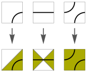
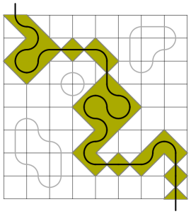
Figure 4: Covering of the defect for $R=R_{1}^{\left(\frac{1}{2},\frac{1}{2}\right)}$ of a sample $8\times 8$ lattice.

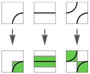
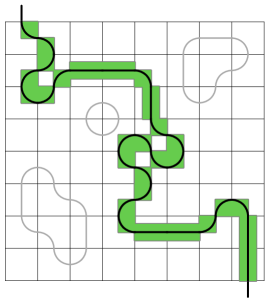
Figure 5: Covering of the defect for $R=R_{2}^{\left(\frac{1}{4},\frac{1}{2}\right)}$ of a sample $8\times 8$ lattice.

As a first example of the various weights given to boxes crossed by the defect, consider boxes with only one quarter-circle or a straight line segment as half-filled, and boxes with two quarter-circles as completely filled. More precisely, if $\epsilon^{2}$ is the area of a tile, then $s_{u}=s_{v}=\frac{1}{2}\epsilon^{2}$ and $s_{w}=\epsilon^{2}$, where $s_{i}$ is the area occupied by an $i$-face. A graphical interpretation of this choice is given in figure 4. If the numbers $H$ and $V$ are even, the defect with maximal $N_{\text{max}}(\epsilon)$ covers the lattice as follows: all boxes not touching the boundary are $w$-faces, while all boundary boxes but one are $u$- or $v$-faces. The last boundary box is necessarily the empty face. We conclude that, for this choice, the linear size $R$ is given by

$$R=\left(HV-H-V+3/2\right)^{1/2}.$$ (22)

More generally, one may define the two-parameter family

$$R_{1}^{\left(a,b\right)}=\bigl{(}2a(HV-H-V+1)+b\bigr{)}^{1/2},$$ (23)

valid when $H$ and $V$ are even, such that $s_{u}=a\epsilon^{2}$, $s_{v}=b\epsilon^{2}$ and $s_{w}=2a\epsilon^{2}$, with $0<a\leq b<2a$. Then $R$ in (22) is simply $R_{1}^{\left(\frac{1}{2},\frac{1}{2}\right)}$. Figure 4 shows the “area” covered by a defect using this correspondence. Note that, unless $a=\frac{1}{2}$, $\epsilon^{2}$ is not in general the area of a box.

One might also be interested in cases where $b\geq 2a>0$. Now the $v$-faces cover a larger area than the $w$-faces, and defects with $N_{\text{\rm max}}$ are found in configurations different from those leading to $R_{1}$. We thus define

$$R_{2}^{\left(a,b\right)}=\bigl{(}2aV+b(HV-H-2V+3)\bigr{)}^{1/2}.$$ (24)

This family of coverings contains the choice $s_{u}=\frac{1}{4}\epsilon^{2}$, $s_{v}=s_{w}=\frac{1}{2}\epsilon^{2}$, or $R_{2}^{\left(\frac{1}{4},\frac{1}{2}\right)}$, depicted in figure 5. We found this covering to be another relevant choice since it can be argued that a quarter-circle is shorter than a straight line segment, and thus that $s_{u}$ should be smaller than $s_{v}$. Because the range of validity of (23) and (24) do not overlap, we might as well define

$$R_{(a,b)}=\begin{cases}R_{1}^{\left(a,b\right)},&0<a\leq b<2a\\[8.53581pt] R_{2}^{\left(a,b\right)},\ &b\geq 2a>0\end{cases}$$ (25)

which is valid as above only when $H$ and $V$ are even numbers, and for the strip only. Although we limited our experiments in what follows to members of (25), one could in principle extend this definition to include the less intuitive situations where $0<b<a$ or $s_{w}\neq 2s_{u}$.

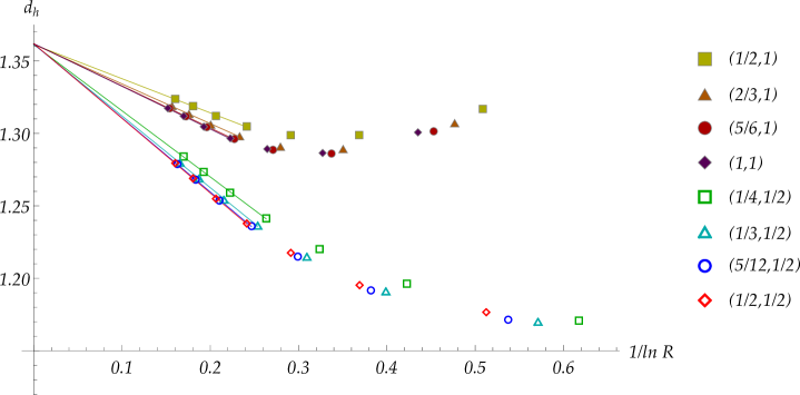
Figure 6: Linear fits of the hull dimension $\widehat{d_{h}}^{H\times V}$ against $1/\ln R$ for different covering definitions using the model $\mathcal{DLM}(3,4)$ on the square geometry. The pair $(a,b)$ refers to $R_{(a,b)}$.

Figure 6 shows fits of the same data obtained from various definitions of $R$. To do these, the numbers of $u$, $v$ and $w$-faces were stored separately for every configuration measured. We see that all the linear fits of $d_{h}$ extrapolate to about $1.362$ at $1/\ln R=0$. The exact value is of no importance right now since these measurements are imprecise and the lattices used are relatively small. It seems clear, however, that $b$ is the important parameter and that, when $b=1$, the $\widehat{d_{h}}^{H\times V}$ values are closer to their asymptotic values. For example, the two curves with $R_{\left(\frac{1}{2},1\right)}$ and $R_{\left(\frac{1}{2},\frac{1}{2}\right)}$ are far apart, but all those with $b=1$ (or $b=1/2$) are bunched together: this probably means that the $v$-faces play a significant role in the length of the defect. Because the results are closer to their asymptotic values for $b=1$, we choose to work with the covering $(a,b)=(1,1)$.

3.2 Technical issues

3.2.1 Simulations on the cylinder

As explained before, the convergence to the asymptotic value of the fractal dimension of the defect is very slow. Despite the improvements made to the algorithm (cf. section A.2), lattices of linear size larger than $H=512$ are difficult to reach. Let us explore the cylindrical geometry using the model $\mathcal{DLM}(3,4)$, where $\beta=1$. Since no loop counting is required in this case, the algorithm is simpler and thus performs more Monte Carlo cycles per second.

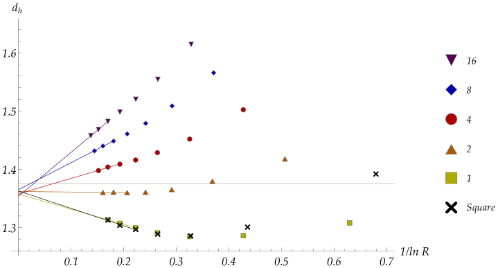
Figure 7: Linear fits of $\widehat{d_{h}}^{H\times V}$ as a function of $1/\ln R$ for cylinders of different $V/H$ ratio and for the square. The horizontal line marks $d_{h}=11/8$ for $\mathcal{DLM}(3,4)$.

We measured the fractal dimension of the defect on cylinders with different aspect ratios $V/H\in\{1,2,4,8,16\}$, where $V$ is the number of boxes along the symmetry axis of the cylinder. The entry and exit points of the defect were set in columns corresponding to the azimuthal angle being $0$ and $\pi$. For each of these ratios $V/H$, the hull fractal dimensions were obtained for $H\in\{4,8,16,32,64,128,256\}$. The plot of linear fits with respect to $1/\ln R$ is shown in figure 7. Obviously, these fits are coarse. Nevertheless, it is already clear that they converge to a narrow window around the predicted value of equation (16), $d_{h}=\frac{11}{8}=1.375$ (horizontal line), as does the curve corresponding to the measurements on the square strip. Still, none seems to aim right at $1.375$. Furthermore, the cylindrical geometry might not speed up the convergence towards the asymptotic value $d_{h}$.

These results call for some discussion. First, the results for the two geometries, that of the strip and of the cylinder, behave quite differently. On the longest cylinder $V/H=16$, the $\widehat{d_{h}}^{H\times V}$’s are significantly higher than $d_{h}=1.375$, as opposed to those of the square geometry which are all lower, except for $H=4$. Second, boundary effects cannot be the only reason for the difference between the two geometries. As discussed in section 3.2.2, significant changes in $d_{h}$ are seen close to the boundary only in a region whose width is a fraction of $H$. Therefore, the long cylinders $V/H=4,8$ and $16$ should have approximately the same $\widehat{d_{h}}^{H\times V}$’s. What we see is probably the effect of configurations with larger and larger winding number. The defect can indeed wrap around the cylinder as it progresses along it. Intuitively, one would think that defects winding, say, twice around the cylinder are longer in average than those with no winding. Because the number of configurations with large winding numbers increases with the ratio $V/H$, a longer cylinder will have defects with larger $\widehat{d_{h}}^{H\times V}$. Third, one might be tempted to do the measurements of $d_{h}$ on cylinders with $V/H=2$, because the measurements for coarse meshes are slightly closer to the predicted value and the slope for larger meshes is small. Of course, if the choice for these cylinders was based on this reason, this would be cheating and it is not clear that the fit over the whole range of $R$ would be any better since it would also require non-linear terms.

3.2.2 Boundary effects and the advantage of the cylindrical geometry

We now explore the effects of the boundary on the measurements of observables. As the lines below will show, it is possible that, in a certain limit, $d_{h}$ might actually be a function of the distance from the boundary. We shall try to give a proper definition of the fractal dimension as a function of this distance, but let us first consider the effect of joining two lattices with different fractal dimensions. Suppose that two square lattices of the same linear size $H$ are covered by different models, $\mathcal{DLM}(p,p^{\prime})$ and $\mathcal{DLM}(q,q^{\prime})$ such that $\frac{p}{p^{\prime}}\neq\frac{q}{q^{\prime}}$, whose defects have dimension $d_{h1}$ and $d_{h2}$, respectively, with $d_{h1}>d_{h2}$. And consider configurations on a new lattice, obtained by joining the two above. Which $\beta$ should give the weight of the loops that overlap the two sublattices? This is a subtle problem and, for the sake of the present argument, it might be enough to confine loops to either sublattices. For sufficiently large $V$ and $H$, the part of the defect in the first half will be of length $c_{1}H^{d_{h1}}$ and $c_{2}H^{d_{h2}}$ in its second half, for some constants $c_{1}$ and $c_{2}$. Thus, its total length is $c_{1}H^{d_{h1}}\left(1+H^{(d_{h2}-d_{h1})}c_{2}/c_{1}\right)$ and the fractal dimension in the whole region is

$$\left.\ln\Bigl{[}c_{1}H^{d_{h1}}\bigl{(}1+H^{(d_{h2}-d_{h1})}c_{2}/c_{1}\bigr{)}\Bigr{]}\right/\ln H\underset{H\rightarrow\infty}{\longrightarrow}d_{h1},$$ (26)

where $R$ is approximated by $H$. Note that this argument can easily be modified to describe two lattices of unequal sizes. This shows a simple fact about fractal dimensions: if a geometric object $S$ is studied on a region $D\subset\mathds{R}^{d}$ of a finite lattice, then its fractal dimension $d_{S}^{D}$ over $D$ will be equal to $d_{S}^{E_{\text{max}}}$, that is to the fractal dimension over the subregion $E_{\text{max}}\subset D$ where it is maximal.

The present situation is slightly more complicated as $d_{h}$ might be varying continuously with the distance from the boundary. What does this mean? The definition (19) applies to a subset $S\subset\mathds{R}^{2}$ or to a subset $S$ of the cylinder as a whole. To define a “local” fractal dimension, consider a cylinder of fixed ratio $r=\text{length}/\text{perimeter}$. Let $L$ be the length of the cylinder and $0\leq l_{1}<l_{2}\leq L$ and let $C_{12}$ be the annulus along (or band around) the cylinder containing points at a distance $l$ from one extremity with $l_{1}<l<l_{2}$. Then one can measure $d_{h}$ on $C_{12}$ by replacing $\mathds{R}^{d}$ with $C_{12}$ in the discussion leading to (19). Numerical estimates of $d_{h}$ can be obtained by covering the cylinder with larger and larger $H\times V$ lattices, with $r=V/H$, and counting the number of intersections of the defect in a given $C_{12}$. Note that the defect can meander out of a given annulus, come back to it, leave again, and so on; all of its intersections with $C_{12}$ must be counted. Unfortunately this fractal dimension $d_{h}=d_{h}(l_{1},l_{2})$ is difficult to measure numerically. The narrowest annulus on the small cylinder $H\times V=8\times 8$ already takes up one eighth of the cylinder’s length. Since the fractal dimension is obtained as an extrapolation over several lattice sizes, the smallest section of the cylinder where this $d_{h}(l_{1},l_{2})$ can be measured effectively is of length $l_{2}-l_{1}=L/8=(V\epsilon)/8$. Unfortunately, some quick explorations have shown to us that a circle at a distance $L/8$ from the boundary is almost free of the boundary effects. The following experiment allows to probe boundary effects.

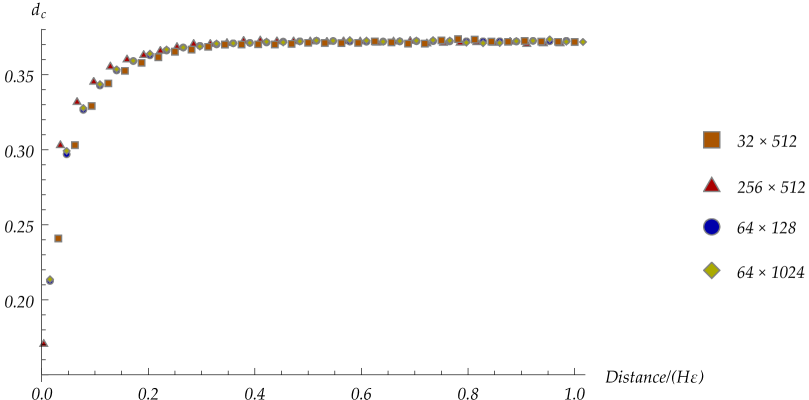
Figure 8: Fractal dimension of the intersections between the defect and circles $C$ on cylinders $(H,V)=(32,512),(256,512),(64,128)$ and $(64,1024)$ for $\mathcal{DLM}(3,4)$.

Let $C$ be a circle at a fixed distance from the boundary of the cylinder. This circle $C$ has (standard or fractal) dimension one. We consider the set $c\subset C$ of intersections of the defect with $C$. The fractal dimension $d_{c}$ of this set is therefore $0\leq d_{c}\leq d_{C}=1$. It is this definition that is used in figure 8 where $d_{c}$ is measured as a function of the distance from the nearest extremity, in units of $H\epsilon$. Cylinders with $(H,V)=(32,512),(256,512),(64,128)$ and $(64,1024)$ were used. All the rows of the cylinders were measured, but only those at a distance $0\leq l\leq H\epsilon$ are shown. Moreover, only a subset of the available data is drawn; the size of the datasets for $64\times 128$ and $64\times 1024$ was reduced by a factor of $2$ while the one for $256\times 512$ was by $8$. Two observations clearly stand out from figure 8: the fractal dimension seems to “feel” the boundary roughly up to a distance of $l/(H\epsilon)=\frac{1}{3}$ and this distance is independent of both the ratio $V/H$ of the cylinder and its mesh size $\epsilon$. The following simple argument relates $d_{c}$ to the fractal dimension $d_{h}$ of the hull.

Let $N(H,V)$ be the number of intersections of the defect with $H$ rows chosen far away from the boundaries of a long cylinder. (We use the notation of section 3.1.) Choose the circle $C$ to be one of these $H$ rows. On average, there will be $N/H$ intersections with this circle $C$ and the fractal dimension $d_{c}$ introduced above is the limit of

$$\frac{\ln(N(H,V)/H)}{\ln R_{C}(H)}$$

as $H\rightarrow\infty$. As before, $R_{C}(H)$ stands for the number of “boxes” necessary to cover $C$. We choose this number to be the maximal number of intersections with $C$, namely $2H-1$. However, $d_{h}$ is the limit of $\ln N(H,V)/\ln R_{H}(H,V)$ where now $R_{H}(H,V)$ is the square root of the maximal number of intersections of the defect with the $H$ rows, that is approximately $\sqrt{2H^{2}}$. So, for large $H$’s, $d_{h}\sim\ln N/\ln H$ and

$$d_{c}=\frac{\ln(N(H,V)/H)}{\ln(2H-1)}\sim\frac{\ln N}{\ln H}-1=d_{h}-1=\frac{\bar{\kappa}}{2}.$$

Since $d_{h}\in[1,2]$, the dimension $d_{c}$ lies in $[0,1]$ as desired and, for $\mathcal{DLM}(3,4)$, $d_{c}$ should be $\frac{3}{8}$, very close to the value $0.37$ seen in figure 8.

This result suggests yet another experiment; one in which $d_{h}$ is measured on the annulus $C_{\text{bulk}}$ which is defined for $l_{1}/L=H/(3V)$ and $l_{2}/L=1-l_{1}/L$, that is, an annulus excluding the region where boundary effects are felt. Figure 9 shows the data for the measurements of $d_{h}$ on $C_{\text{bulk}}$ for cylinders with ratios $V/H\in\{1,2,4,8\}$. There are four other sets of points all converging to the same value, around $1.35$. These are the measured $\widehat{d_{h}}$ on the complement $C_{\text{boundary}}$ of $C_{\text{bulk}}$ in the cylinder. Results remain preliminary as they are limited to $H\leq 256$ only. But they are striking. The finite fractal dimensions on $C_{\text{bulk}}$ all converge quite close to the expected $\frac{11}{8}$ and all those on the complement to another lower value. These results do not allow us to determine whether the fractal dimension on $C_{\text{boundary}}$ and that on $C_{\text{bulk}}$ are distinct. Indeed, in figure 8, the points for the largest lattice ($256\times 512$) clearly stand over those of the other lattices when the circle $C$ is chosen close to the boundary. They seem to indicate that the limit of $d_{c}$ is not yet reached. But even if these two fractal dimensions on $C_{\text{boundary}}$ and $C_{\text{bulk}}$ were the same, these results do allow to conclude that the rate of convergence to their asymptotic value is different. This is the main conclusion of this long analysis.

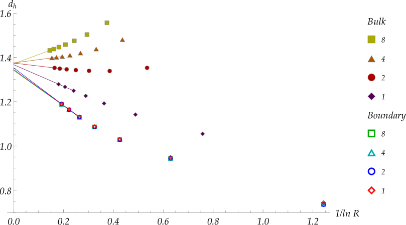
Figure 9: Measurements of $C_{\text{boundary}}$ and $C_{\text{bulk}}$ on cylinders with $V/H=1,2,4$ and $8$.

Figure 9 shows how to measure efficiently any $d_{S}$ in the bulk whenever the rate of convergence of $d_{S}^{H\times V}(l)$ depends on the distance $l$ from the boundary. If we assume that the function $d_{S}^{H\times V}(l)$ is approximately conformally invariant, then the effects of the boundary will be definitely more important for measurements on the square. To see this, map conformally the cylinder onto the disk by the exponential. Because the circumference of the cylinder has $H$ sites, the annulus that is at distance $H/3$ from the extremity will be sent onto a circle with radius $r\sim e^{-2\pi/3}\,r_{\text{disk}}<0.125\,r_{\text{disk}}$. The Schwarz-Christoffel map that sends the disk onto the square will change slightly the form of this inner circle close to the center, but it will not change the fact that a minute number of boxes of the square geometry actually lie in the bulk (see Langlands et al. [17]), approximately one hundredth of the total number of boxes. This precludes obtaining a good measurement of $d_{S}$ in the bulk using square geometries. Indeed, even for a $256\times 256$ lattice, one would have to count the intersections of the defect with a small square at the center of the lattice of about $30\times 30$ boxes.

We therefore propose to restrict our study to the fractal dimension $d_{S}$ in the bulk, and use the cylindrical geometry to measure it, with cylinders of ratio $V/H=2$. For simplicity and to minimize boundary effects in our experiments, we define the bulk as the region enclosed by the annuli at distance $l_{1}=H/2$ and $l_{2}=3H/2$ from one of the extremities of the cylinder. To extend the discussion in section 3.1, we must seek the maximum number $N_{\text{\rm max}}$ of intersections the defect can have with this bulk section. Again we assume that faces $u$ and $v$ count for one intersection and $w$ for two. For $(a,b)=(1,1)$, the most dense configuration has $H(2H-1)$ such intersections and we define $R$ to be the square root of this number. This choice of the size ratio $V/H=2$ and bulk region allows to use half of the boxes for measurements with only a reasonable increase in the total number of boxes. This seems to be a good compromise.

3.2.3 The distribution of the winding number

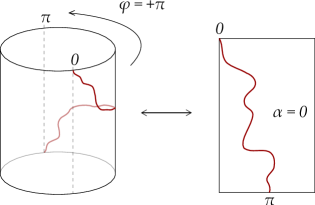
(a) Winding number $\alpha=0$.

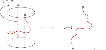
(b) Winding number $\alpha=1$.

Figure 10: Sample configurations with winding numbers $\alpha=0$ and $\alpha=1$.

Recall that the entry and exit points of the defect are chosen to be at locations corresponding to azimuthal angles equals to $0$ and $\pi$, respectively. We define the winding number $\alpha$ of the defect by

$$\alpha(\varphi)=\frac{\pi-\varphi}{2\pi},$$ (27)

where $\varphi$ is the azimuthal angle of the defect. A configuration will be said to have winding number $\alpha=0$ if the angle of the defect $\varphi$ has increased by $\pi$ while going from one extremity to the other. Note that, with this definition, a variation of $-\pi$ of the angle would amount to a winding number $\alpha=1$. Two sample configurations having winding numbers $0$ and $1$ are shown in figure 10. The definition (27) is asymmetric, and rather unpleasant. However, as will be seen soon, this asymmetry is actually welcome. The simulations reported in the previous paragraphs 3.2.1 and 3.2.2 were done starting the thermalization with a defect with zero winding number. This has the consequence that no configurations with odd winding numbers are considered in the Monte Carlo integration. Indeed, the upgrade algorithm (section A.1) always changes the winding number by zero or two units. For example, in figure 11, the flip of the gray box changes the winding number from $0$ to $2$.

Figure 11: The algorithm preserves the parity of the winding number.

The exclusion of all configurations with an odd winding number is a serious problem. One could try to overcome it by measuring separately the distributions of the defect’s length for configurations with even and for those with odd winding numbers. For the latter, it would amount to start with a configuration in this set. But then the determination of the distribution of the defect length for the whole space of configurations would raise the question of the relative probability of the two sets and this seems extremely difficult. As it turns out, this problem does not occur! Indeed, the probability distribution of the winding number is obviously invariant through a mirror containing the cylinder axis, corresponding to $\varphi\rightarrow-\varphi$. Due to our definition, however, this symmetry sends a configuration with winding number $0$ onto a configuration with winding number $1$. More generally, configurations with winding number $\alpha$ are sent onto configurations with winding number $1-\alpha$ and are therefore equiprobable. Note that, if the entry and exit points had been put in the same column, that is with the same azimuthal angle, the problem of discarding the odd or the even configurations would have been a serious one.

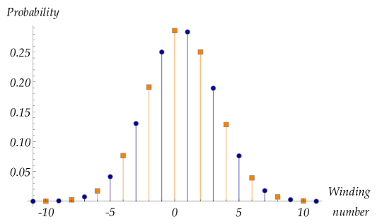
Figure 12: The discrete probability density of the winding number on the $V/H=16$ cylinder for $\mathcal{DLM}(3,4)$.

Figure 12 shows the probability density function of each winding number within its set, either even (square dots) or odd (disks), measured on the cylinder with ratio $V/H=16$ and $H=8$ for the model $\mathcal{DLM}(3,4)$. It supports quite nicely the previous observation, as the two histograms are mapped onto one another by the symmetry $\alpha\leftrightarrow 1-\alpha$. It is interesting to note also that quite large winding numbers are reached. The histogram box for $10$ is readable, but larger winding numbers were also reached. Pinson [21] and Arguin [2] have considered the probability of Fortuin-Kasteleyn configurations having a given homotopy on the torus. Their results may be applicable to long cylinders or, at least, give a reasonable prediction for this geometry.

4 Results

To estimate the fractal dimension of the hull for a given lattice size, we took $m$ measurements, usually with $m=10\,000$, of the length $L$ of the defect in the bulk region of the $V/H=2$ cylinder. Each pair of consecutive measurements is separated by a fixed number $\Delta$ of Monte-Carlo iterations which varies according to the size of the lattice and the model itself. This procedure was carried out simultaneously on $n$ machines, with $n\geq 20$, and for cylinders with $H=8,16,32,64,128,256,512$. The average fractal dimension of a given cylinder of size $H$ is then obtained by averaging the defect’s length $N(H,V)=L$ of equation (21) over all the $m\times n$ data:

$$\widehat{d_{h}}=\frac{1}{mn}\sum_{j=1}^{n}\sum_{i=1}^{m}\frac{\ln L_{i,j}}{\ln R(H)},$$ (28)

where $R(H)=\bigl{(}2H^{2}-H\bigr{)}^{1/2}$ in the bulk for the cylinders with $V/H=2$. The same procedure was used for the external perimeter. A typical dataset obtained by this method is shown in table 2.

$H$	$8$	$16$	$32$	$64$	$128$	$256$	$512$
$\widehat{d_{h}}$	$1.2772\bigl{|}\bigr{.}6$	$1.2923\bigl{|}\bigr{.}4$	$1.3045\bigl{|}\bigr{.}4$	$1.3143\bigl{|}\bigr{.}4$	$1.3215\bigl{|}\bigr{.}5$	$1.3279\bigl{|}\bigr{.}7$	$1.3323\bigl{|}\bigr{.}4$

Table 2: Hull fractal dimension measurements for $\mathcal{DLM}(3,4)$ on cylinders $H={8,16,32,64,128,256,512}$ with $V/H=2$. The notation $1.2772\bigl{|}\bigr{.}6$ means that the $95\%$ confidence interval’s half width is $0.0006$ and centered on $1.2772$.

model name, $\mathcal{DLM}(p,p^{\prime})$	$\bar{\kappa}$	$\beta$	$d_{h}=d_{ep}$	$\widehat{d_{h}}$	$\widehat{d_{ep}}$
percolation, $\mathcal{DLM}(2,3)$	$\frac{2}{3}$	$0$	$\frac{4}{3}\simeq 1.3333$	$1.3328\bigl{|}\bigr{.}13$	$1.3332\bigl{|}\bigr{.}19$
Ising, $\mathcal{DLM}(3,4)$	$\frac{3}{4}$	$1$	$\frac{11}{8}=1.3750$	$1.3757\bigl{|}\bigr{.}13$	$1.3751\bigl{|}\bigr{.}15$
tricritical Ising, $\mathcal{DLM}(4,5)$	$\frac{4}{5}$	$\sqrt{2}$	$\frac{7}{5}=1.4000$	$1.4025\bigl{|}\bigr{.}14$	$1.3986\bigl{|}\bigr{.}19$
3-Potts, $\mathcal{DLM}(5,6)$	$\frac{5}{6}$	$\frac{1}{2}\bigl{(}1+\sqrt{5}\bigr{)}$	$\frac{17}{12}\simeq 1.4167$	$1.4197\bigl{|}\bigr{.}11$	$1.4119\bigl{|}\bigr{.}12$
4-Potts, $\mathcal{DLM}(1,1)$	$1$	$2$	$\frac{3}{2}=1.5000$	$1.5021\bigl{|}\bigr{.}12$	$1.4615\bigl{|}\bigr{.}10$
$\mathcal{DLM}(5,7)$	$\frac{5}{7}$	$\frac{1}{2}\bigl{(}\sqrt{5}-1\bigr{)}$	$\frac{19}{14}\simeq 1.3571$	$1.3592\bigl{|}\bigr{.}20$	$1.3586\bigl{|}\bigr{.}26$

Table 3: Extrapolated fractal dimensions for the hull and external perimeter. Fits of the form $\beta_{0}+\beta_{1}/\ln R+\beta_{2}/\ln^{2}R+\beta_{3}/\ln^{3}R$ were considered and model testing led us to set $\beta_{2}=0$ (see section B.2.3).

The extrapolated fractal dimensions of the hull and external perimeter for all models studied are shown in table 3 with their 95% confidence interval. The meaning of our confidence interval is as follows: if the experiment was repeated many times, then an average of $5$ fits out of $100$ would predict an average value $\widehat{d}$ at $1/\ln R\to 0$ that lies outside the $95\%$ confidence interval of table 3. We see that the extrapolations are in good agreement with the theoretical values given by equations (16) and (17). Still, some of the confidence intervals do not contain the theoretical values; this is especially true for the external perimeter in $\mathcal{DLM}(1,1)$. Even though the definition of the confidence interval does not imply that it should contain the theoretical value with $95\%$ probability, one would like to better understand these small departures. These discrepancies for the hull and the external perimeter will be discussed in the next subsections.

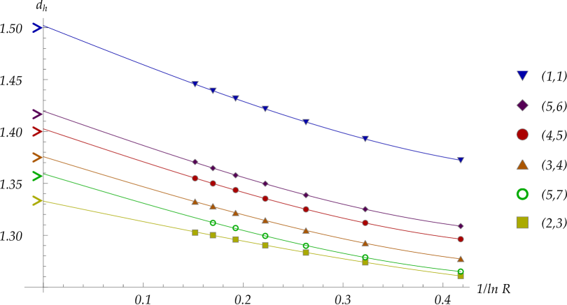
Figure 13: Measurements of the hull’s fractal dimension against $1/\ln R$, and the corresponding fits on the $V/H=2$ cylinder. The theoretical values are designated by wedges at $1/\ln R\to 0$. The pair $(p,p^{\prime})$ refers to $\mathcal{DLM}(p,p^{\prime})$.

4.1 The hull

The measurements and fits of the hull’s fractal dimension are shown in figure 13 for all models. The error bars are much smaller than the symbols used to depict the data. According to the statistical test used (see appendix B.2), the best fits are obtained for the model $Y(R)=\beta_{0}+\beta_{1}/\ln R+\beta_{3}/\ln^{3}R$, where $\beta_{1}$ and $\beta_{3}$ are real constants, $R$ is the linear size of the lattice, and $\beta_{0}$ is a real constant to be interpreted as the fractal dimension. Note that the necessity of a quadratic term in $1/\ln^{2}R$ is always rejected by the statistical analysis. We do not have a straightforward explanation for this. The figure underlines the quality of the match between theoretical values (16) and measured ones and also reveals some of the possible difficulties.

First and foremost, the data show that the $\widehat{d_{h}}$’s, as functions of $1/\ln R$, are not linear and have large slopes. The smallest lattice used in the fits has $H=8$. On the interval of $H$ covered by our measurements, just a little more than half the distance between $\widehat{d_{h}}^{H=8}$ and the theoretical value is covered. More precisely, the ratio of the data span $\bigl{|}\widehat{Y}\bigl{(}R(512)\bigr{)}-\widehat{Y}\bigl{(}R(8)\bigr{)}\bigr{|}$ over the distance $\bigl{|}d_{h}-\widehat{Y}\bigl{(}R(8)\bigr{)}\bigr{|}$, averaged over all fits, is only $0.57$. Even with data for larger lattices, say $H=1024,2048$ and $4096$, this ratio would still be under $0.7$. These extrapolations are obviously difficult. Second, the fits are extremely sensitive to the non-linear terms of $Y(R)$. According to table 3 and figure 13, the fits give an extrapolated fractal dimension that slightly overshoots the theoretical one, the only exception being the fit for $\mathcal{DLM}(2,3)$. The fit for $\mathcal{DLM}(3,4)$ overshoots very slightly, by about $0.0007$, and the others by about $0.002$. The latter are precisely those whose graphs are the most curved. The departure from the predicted values is even more striking for some values of the external perimeter and we shall propose in the next subsection an experiment to better understand the systematic error caused by the extrapolation.

Of course, better estimates of $d_{h}$ would require data for larger lattices. For our algorithm, the major obstacles to reach these lattices are the following. First, the smaller the $u$, $v$ and $w$ weights (see (2.1.2)), the slower the simulations. The reason is that, when the algorithm steps on an empty $3\times 3$ block, the probability that the block remains empty ranges from $90$% for $\mathcal{DLM}(1,1)$ to over $99$% for $\mathcal{DLM}(5,7)$. Because the functions $u$, $v$ and $w$ increase with $\beta$, the autocorrelation function of the Monte Carlo chain decreases faster for larger $\beta$, as there is less emptiness. Second, the dependency of $d_{h}$ on boundary effects favored simulations on the cylinder. But accounting for the cyclical boundary conditions slows the algorithm by about $5\%$. Third, the amount of data on the lattices up to $H=256$, for $\beta\neq 0,1$, are easily stored in the cache of the cpus used but, as $H$ reaches $512$, more traffic between the cache and the memory is needed as seen by the sudden decrease in the number of Monte Carlo cycles performed per second for these larger $H$ values. Finally, the model $\mathcal{DLM}(5,7)$ is the hardest to measure. As seen in figure 13, $H=256$ is the largest lattice for it. Its fugacity $\beta_{(5,7)}\simeq 0.6180$ is the lowest among the models measured, excluding $\beta_{(2,3)}=0$ that has its own algorithm anyway. The $u$, $v$ and $w$ are small and the cost of creating a loop starts to show, leading to rather empty configurations with the problem noted above.

4.2 The external perimeter

The definition we used for the external perimeter is inspired by the biased walker of Grossman and Aharony [15] and its variant for loop models introduced in Saint-Aubin et al. [23]. Starting at one end of the cylinder, the walker follows the left side of the defect all the way down to the other extremity of the cylinder and, in the meanwhile, counts a unit of length each time it encounters a $u$- or $v$-face. When it encounters a $w$-face made up of two quarter-circles coming from the defect, it still counts a unit of length, but then it does not enter the fjord created at that point, unless the two quarter-circles possess azimuthal angles $\varphi_{1}$ and $\varphi_{2}$ such that $\lvert\varphi_{1}-\varphi_{2}\rvert=2\pi$. (See section 3.2.3 for the definition of $\varphi_{i}$.) That is, if we interpret the defect as a chordal SLE growing from one end of the cylinder to the other, then its azimuthal angle as it progresses along the trajectory takes the value $\varphi_{1}$ when it first crosses the $w$-face and $\varphi_{2}$ the second time. The only possible differences of these two values are $\lvert\varphi_{1}-\varphi_{2}\rvert=0$ and $2\pi$. When the difference is $2\pi$, we consider that this $w$-face is not the entry point of a fjord because otherwise the walker would return to its starting point without scanning the defect in its entirety. The external perimeter for two distinct defects is drawn in figure 3.

As observed in [23], there could be more than one definition for the external perimeter in loop models. Thus, to confirm the validity of the one chosen, we have compared the extrapolated value obtained for the dense phase of $\mathcal{DLM}(2,3)$ with that of $\mathcal{LM}(2,3)$, previously measured in [23]. Since the two models belong to the same universality class, as explained in section 2.2, the two extrapolations should be equal. For $\mathcal{DLM}(2,3)$ with the above definition, we measured $1.3368$, while one finds $1.326$ for $\mathcal{LM}(2,3)$ in [23]. Both measures are fairly close to each other and to the theoretical value of $d_{ep}=4/3$. We thus conclude that there is no reason to doubt our definition.

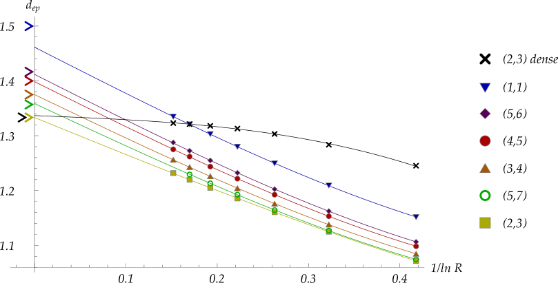
Figure 14: Measurements of the external perimeter’s fractal dimension, and the corresponding fitted curves, for all the previously cited models on the $V/H=2$ cylinder. The pair $(p,p^{\prime})$ refers to $\mathcal{DLM}(p,p^{\prime})$.

The measured dimensions $\widehat{d_{ep}}$ for the external perimeter are shown in table 3. Again, we see that the agreement with the prediction is generally good, although the results for $\mathcal{DLM}(5,6)$, and particularly the one for $\mathcal{DLM}(1,1)$, are farther away from the theoretical ones than the corresponding results of the hull. Nevertheless, as visible in figure 14, the fits are good enough to confirm convincingly the theoretical predictions of equation (17), except maybe for $\mathcal{DLM}(1,1)$. The latter model is in the equivalence class with central charge $c=1$ to which also belongs the $4$-Potts model. It is known that, for many models at $c=1$, the scaling of geometric objects include logarithmic terms (see for example [1]) and thus extrapolation is predictably difficult for $\mathcal{DLM}(1,1)$. Still, one would like to better understand the systematic undershooting for this geometric exponent and, to a lesser extent, for that of the hull. We propose the following experiment with this goal in mind.

To the Monte Carlo data for $\mathcal{DLM}(1,1)$ and $\mathcal{DLM}(5,6)$ that we have, we added the point $(1/\ln R,d_{ep})=(0,d_{ep}^{\text{\rm theo}})$, i.e. the theoretical prediction. (This idea is not new. For example, Asikainen et al. [3] also use fits where the theoretical fractal dimensions appear explicitly to determine their error bars.) And we fitted the new datasets with this single additional point. According to the $F$-test (see appendix B.2.3), it is now appropriate to keep both of the terms $1/\ln^{2}R$ and $1/\ln^{3}R$, and the coefficients of $Y(R)=\beta_{0}+\beta_{1}/\ln R+\beta_{2}/\ln^{2}R+\beta_{3}/\ln^{3}R$ are now all significant. Visually the two fits, with and without the theoretical value, are barely distinguishable in the range of measurements as can be seen in figure 15, but they split quickly to the left of the datum corresponding to the largest lattice. We therefore propose the following simple interpretation for the systematic departure from the predicted values: in the range $H\leq 512$, the cubic term $1/\ln^{3}R$ is large enough to conceal the quadratic one. Without the additional (predicted) point, the $F$-test says that the hypothesis that $\beta_{2}$ is zero cannot be rejected. (Actually, if one includes $\beta_{2}$, the $\widehat{d_{h}}$ is similar, but the confidence interval is larger.) The fit with only $Y(R)=\beta_{0}+\beta_{1}/\ln R+\beta_{3}/\ln^{3}R$ is then excellent. But, with the predicted value added, the hypothesis that $\beta_{2}$ is zero must be rejected and the new fit goes through all the measured $\widehat{d_{h}}^{H\times V}$ with equal precision. We made one further check by adding, instead of the theoretical value, a set of random points at $1/\ln R=0.05$ and $0.10$ whose averages sit on the new fits of figure 15 with a variance similar to the spread of the data at $H=512$. The fit with these random points had the same properties as the one with the theoretical value added. The conclusion seems to be that the sizes of lattice we used do not allow to measure properly both $\beta_{2}$ and $\beta_{3}$ that describe finite-size corrections from $H\simeq 8$ to $H\rightarrow\infty$. The values $1/\ln R=0.05$ and $0.10$ correspond to lattices of size $H\simeq 3\times 10^{8}$ and $2\times 10^{4}$. They are out of reach with our algorithms!

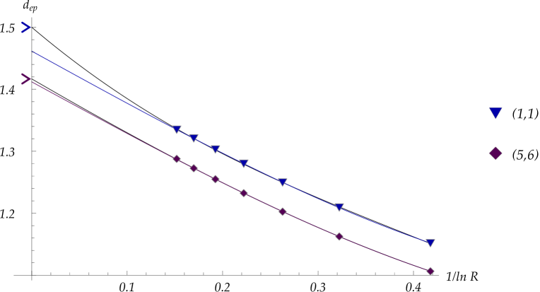
Figure 15: Fits and measurements for the external perimeter of $\mathcal{DLM}(5,6)$ and $\mathcal{DLM}(1,1)$ as well as the fits with the additional point $d_{ep}^{\text{\rm theo}}$ at $1/\ln R=0$.

4.3 The red bonds

$H$	$8$	$16$	$32$	$64$	$128$	$256$
$\widehat{d_{rb}}$	$0.1315\bigl{|}\bigr{.}5$	$-0.0243\bigl{|}\bigr{.}4$	$-0.1262\bigl{|}\bigr{.}7$	$-0.1991\bigl{|}\bigr{.}9$	$-0.2510\bigl{|}\bigr{.}11$	$-0.2941\bigl{|}\bigr{.}21$

Table 4: The measured fractal dimension of red bonds for the Ising model $\mathcal{DLM}(3,4)$ on cylinders $H={8,16,32,64,128,256}$ with $V/H=2$.

To measure the fractal dimension of red bonds, we use two defects, instead of just one, so that the domain between them is interpreted as a proper “cluster”. The fractal dimension is then computed by finding the number of $w$-faces visited by both defects and multiplying this number by two (see section 2.3). The measurement of this observable is difficult since, for models in the dilute phase, not even all configurations have at least a single red bond. Moreover, the average number of red bonds is smaller than $1$. Because of this, the fractal dimension cannot be estimated using equation (28) and we used an alternative definition that was also used in Saint-Aubin et al. [23]:

$$\widehat{d_{rb}}=\frac{1}{n}\sum_{j=1}^{n}\frac{\ln\overline{N_{j}}}{\ln R(H)},$$ (29)

where $\overline{N_{j}}=\frac{1}{m}\sum_{i=1}^{m}N_{i,j}$ and $N_{i,j}$ is the number of red bonds of the $i$-th datum in the $j$-th Markov chain. The numbers $m$, $n$ and $R(H)$ have the same meaning as in section 4.1.

As the data of table 4 attest, there are less and less red bonds in average for each lattice configuration as $H,V\to\infty$. Because of this, we restricted our measurements to $\mathcal{DLM}(3,4)$, as it has the most efficient algorithm, and confined the lattices to $H\in[8,256]$. The difficulty is well illustrated by the following numbers: the average value $-0.2941\pm 0.0021$ at $H=256$ in table 4 required a total of about $10^{15}$ Monte Carlo iterations, excluding the number of iterations needed for an adequate thermalization of the startup lattices. By comparison, the result $1.3323\pm 0.0004$ at $H=512$ for the hull required about the same number. In other words, obtaining a measurement for the hull at $H=256$ with a similar confidence interval of $\pm 0.002$ would require only about $5.5\times 10^{12}$ iterations, i.e. approximately $1/180$ times the number required in the red bonds experiment.

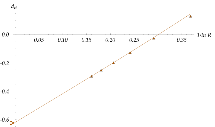
Figure 16: Measurements of the red bonds’ fractal dimension and its corresponding fit, for the dilute Ising model $\mathcal{DLM}(3,4)$ on the $V/H=2$ cylinder.

Although some of the measurements are less precise than for the other observables, we obtained the extrapolated $\widehat{d_{rb}}=-0.621\pm 0.004$, in good agreement with the predicted value $d_{rb}=-0.625$ (eq. (18)). This result is surprisingly close to the theoretical value, considering the extreme extrapolation that had to be done: the value at $H=256$ remains at about $0.33$ from the theoretical prediction, that is $10$ times farther than the corresponding value was for $d_{ep}$ in $\mathcal{DLM}(1,1)$. However, the fit gives a good result because the curvature is gentler, and the discrepancy from linearity is rapidly wearing off as $1/\ln R$ decreases. The average values as well as the fit for this observable have been plotted in figure 16.

The negative fractal dimension $d_{rb}$ is somewhat of a novelty here, but can be easily interpreted. As the lattice size grows, the average number of times the two defects touch one another decreases toward zero, and the rate of this decrease is measured by the negative fractal dimension $d_{rb}$.

5 Concluding remarks

The agreement between the theoretical values and the measured ones (table 3) is very good. It is similar in precision to that obtained in [23] for the dense models, or even slightly better. Note that the difficulties that had to be overcome for the dilute models were quite different from those encountered for the dense ones. The improved quality of the geometric exponents obtained here might stem partially from a more systematic and finer statistical analysis (see appendix B).

The proposed upgrade algorithm for the dilute models, and its variants for the models with $\beta=0$ and $1$, was quick enough to provide very precise measurements for lattice sizes up to $H\times V=512\times 1024$. Still, one feels that, unless willing to wait for the next or the second next generation of cpus, the algorithm proposed here has reached its practical limits. New methods, in the direction of those proposed by Deng et al. [8], will be necessary to probe further these models.

Appendix A Upgrade algorithms

In this appendix, we first present the upgrade algorithm common to all the models. The subsequent subsections sketch the ideas relevant for particular models.

A.1 The basic algorithm

For the dense loop models $\mathcal{LM}(p,p^{\prime})$, reviewed in appendix C, each box is in either one of two faces, corresponding to the two $w$-faces of $\mathcal{DLM}(p,p^{\prime})$. A straightforward Metropolis-Hastings upgrade can be chosen as simply changing one box at a time and checking whether the usual Monte-Carlo condition is verified. (See [23].) For the dilute loop models $\mathcal{DLM}(p,p^{\prime})$, the edges of the nine possible states are not necessarily crossed by loop segments, as is shown in figure 1. Indeed, the empty state contains no loop segments, two edges of the $u$- and $v$-faces are crossed by a loop segment and all four edges of the $w$-faces are crossed. As the loop segment must remain continuous at box interfaces, we could refine the previous algorithm by requiring that the edges that are crossed before the change, and only those, remain crossed after the change. But then the only effective change would be the flipping of a $w$-face to its mirror face, thus preventing the algorithm from sampling over all configuration space. Because of this, we are forced to consider changing many contiguous boxes in a single upgrade step.

The upgrade step must therefore change an $m\times n$ block of boxes, with $m,n\geq 2$. First an $m\times n$ block is chosen at random in the $H\times V$ lattice on the cylinder. Because this block has to fit entirely in the lattice, this amounts to placing randomly the upper left box of the block in the first $V-n+1$ rows, all possibilities being weighted uniformly. Second, the content of the $m\times n$ block is changed for another admissible block. To be admissible, the $2(m+n)$ edges of the block must be crossed by a loop if they were in the original block, and be free of crossing if the original edge had none. For instance, if the chosen $3\times 3$ block corresponds to figure 17(a), then an admissible replacement is shown in figure 17(b), while figure 17(c) shows a forbidden replacement block. The new block must be chosen uniformly among admissible ones. Finally, the Boltzmann weight $u^{n_{u}}v^{n_{v}}w^{n_{w}}\beta^{N}$ of the configuration where the $m\times n$ block is replaced by the new choice is computed and compared with the original one (see (6)): the Metropolis-Hastings ratio decides whether the replacement is to be accepted or rejected. Note that, even though the change is limited to the block, the computation of the weight involves counting the number of closed loops (except when $\beta=1$) and might therefore require exploring the configuration at a large distance of the $m\times n$ block under consideration.

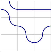
(a) The chosen block.

(b) An admissible replacement block.

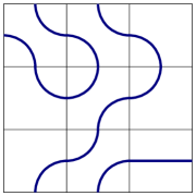
(c) A forbidden replacement block.

Figure 17: The original $3\times 3$ block in (a) with an admissible replacement in (b) and a forbidden one in (c).

The requirement of uniformity of the block state among admissible ones raises a subtle problem. One might think that it is achieved by simply choosing the face of each of the $m\times n$ boxes one after the other, respecting at each step the conditions on the perimeter. This is not the case as the next example shows. Suppose that the $m=n=3$ block to be changed is that of figure 17(a) and that the new box states will be chosen from left to right, top to bottom. If the first box to be chosen is the upper left one, three choices are admissible: the $u$-face $u_{2}$ that has a single west-north crossing, and both $w$-faces $w_{1}$ and $w_{2}$. (As in section 2.1.2, the index of the letters $u$, $v$ and $w$ refers to the order of figure 1, the bottom box being labeled by $1$.) Each of these three faces will be given probability $\frac{1}{3}$. It is easy to check that there are two possible replacements for the next box, and only one for the last box of the top row. Similarly, two faces are admissible for the leftmost box of the second row. So far, twelve different fillings are possible, each occurring with probability $\frac{1}{12}$.

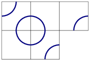
Figure 18: If we chose the face of each box sequentially, then the left block would be more probable than the right one.

The difficulty occurs for the box at the center. Two of the twenty-seven possible fillings are shown in figure 18. For the filling on the left, two choices are allowed: the $u_{4}$ or the empty face. But for the filling on the right, three are possible, namely the $u_{2}$, $w_{1}$ and $w_{2}$ faces. This means that, starting from the center box, the blocks obtained from the filling on the left will occur with probability $\frac{1}{24}$, and the ones obtained from the right filling will get probability $\frac{1}{36}$: this violates the requirement of uniformity. To assure uniformity, one has to determine first, for a given block, the number of allowed replacements. We found it more efficient to count beforehand these for all the possible edge configurations of the perimeter, or boundary state, for the $m\times n$ block, and actually construct a list of the admissible replacements. For $m=n=3$, there is a total of $113\,361$ possible replacements for the $2048$ boundary states. Depending on the boundary state, there can be as little as $18$ admissible replacements or as many as $690$.

We decided to work with $3\times 3$ blocks. The list of possible replacements for larger blocks would take up much more memory. Moreover, given some boundary state on the block being changed, the variations in probability brought by tentative replacements would likely be in a wider range and lead to a higher rejection rate. Such an argument does not hold for $2\times 2$ blocks, the smallest that allow exploration of the whole configuration space, for which the list of replacements is short and the acceptance rate is high. However, some experimentation with this shorter list shows that the autocorrelation between upgrades, and therefore the number of upgrades between statistically independent measurements, is very high. We found the $3\times 3$ blocks to be a good compromise.

A.2 Improvements

The Ising model is described by the dilute phase of $\mathcal{DLM}(3,4)$. Since the loop fugacity of this model is $\beta=1$, there is no need to know the number of loops crossing the $m\times n$ block when computing the Boltzmann weight. This simplification greatly speeds up the algorithm because loop counting is by far its most time-consuming component.

It is more difficult to improve the algorithm for models with $\beta\in(0,2]\setminus\{1\}$. The rest of this paragraph is devoted to this problem, while the case $\beta=0$ will be discussed in subsection A.3. One can distinguish between models according to whether $0<\beta<1$ or $1<\beta\leq 2$, because models of the first type will tend to be filled with less loops than those of the second type. Most configurations of both types of models have large loops, some being of length of the same order as that of the defect.

Our first attempt to compute Boltzmann weights was rather naive. We simply followed every connected path that crosses the $m\times n$ block until it returns to its starting point or, if the path is part of the defect, reaches the boundary of the lattice; that works, but it is slow, especially for large lattices. It is slow due to the presence of the defect and, potentially, of long loops. The problem is particularly acute for those models with large $\beta$, e.g. the dilute phase of $\mathcal{DLM}(1,1)$, because the predicted hull fractal dimension of the defect is large and lots of loops are present.

A way of reducing the impact of the defect crossing the $m\times n$ block is to assign a time order to each edge it crosses, starting from its entry point down to its exiting point. Because every edge crossed by the defect is then identified in some way as belonging to it, it is possible to distinguish the defect from a loop during loop counting. Moreover, the time ordering allows to identify when the defect enters first the block and when it leaves it for good. Since these two edges cannot change when going from the original to the replacement block, it allows for quick identification of those situations where the defect generates a loop or absorbs one intersecting the block.

Large loops are common, some with size commensurate to that of the defect. When the $m\times n$ block selected for the upgrade is crossed by one of these, a slowing down of the algorithm similar to that encountered for the defect is observed. To get over this problem, we time-ordered the edges of each loop, starting from an arbitrary edge on its path, and also assigned a unique number to each loop. During the loop counting phase of the former block, the number of different loops crossing the block is now obtained very quickly: it is simply the total of different loop numbers. The time order is useful because it allows the algorithm to know how the different edges of the same loop or defect are connected to each other outside the $m\times n$ block. Like for the entry and exit points of the defect, those external connections will not change after replacement of the $m\times n$ block. So, with this information, during the loop counting step for the replacement block, the algorithm does not have to follow the path of the loops (or defect) which lies outside the block since the reentry point is now known.

A.3 The case $\beta=0$

The percolation model, as described by the dilute phase of $\mathcal{DLM}(2,3)$, needs a special algorithm to be simulated efficiently since its $\beta=0$ loop fugacity forbids the presence of loops. It is still possible to choose an $m\times n$ replacement block on the sole basis that it suits the boundary conditions of the block, but then if the chosen configuration creates a loop, this choice will have to be rejected. To get rid of this problem, we need to know what the external connections of the block are, as described in section A.2; this information is easily retrieved if the defect is time-ordered. All that is left to do is to choose, with uniform probability, a replacement amongst the blocks respecting both the boundary conditions and external connections. In figure 19, an example of a possible replacement admitting no loop is shown for a $3\times 3$ block on a lattice with cylindrical geometry.

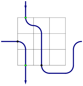
(a) The block to replace.

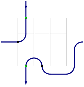
(b) An admissible replacement.

Figure 19: A possible transition for a $3\times 3$ block on the cylinder yielding no loop. The first and last boundary edges crossed by the defect are marked by pale dots, while the remaining connected edges are marked by black ones.

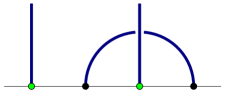
Figure 20: Diagrammatic representation of the external connections shown in figure 19. The points are aligned by starting from the top left edge and following the boundary clockwise.

To obtain a new list of replacement blocks appropriate for this model, the external connections of the $m\times n$ block have to be taken into account, so it is necessary to be able to enumerate them all. To do so, one may use a diagrammatic representation, an example of which can be seen in figure 20. This example of a diagram corresponds to the external connections of figures 19(a) and 19(b). Under this representation, the connected edges are linked pairwise by arches, and the entry and exit edges of the defect in the block, depicted by pale dots in the figures, are linked at infinity by vertical lines. The linking arches may not cross each other, but they may go “under” the vertical lines, that is without intersecting them, as the defect may wind around the cylinder without self-intersecting. For given block boundary conditions, consisting of $p$ connected and $2m+2n-p$ unconnected edges, there are

$$E_{p}=\frac{1}{2}p(p-1)C_{p-2},$$ (30)

different external connections, where $C_{i}=\binom{i}{i/2}-\binom{i}{i/2-1}$. To obtain the new list of replacements, one must first fix the boundary conditions and external connections of the $m\times n$ block and then, using the list of section A.1, check whether any of the suggested replacements yields loops; those that do not generate loops belong to the new list. This testing has to be repeated for all possible external connections matching these fixed boundary conditions. Finally, repeating this process for all $2048$ boundary conditions completes the list of replacements. For a $3\times 3$ block, we find, using equation (30), a total of

$$N=\sum_{\begin{subarray}{c}i=2\\ i\;\text{even}\end{subarray}}^{12}\binom{12}{i}E_{i}=144\,408$$

different external connections, leading to a list of over $3.8\times 10^{6}$ replacements. This is to be compared with the $113\,361$ possible replacements of the standard $\beta>0$ list.

When the $\beta=0$ algorithm steps on an empty $m\times n$ block, nothing can be done since loops are not allowed, and so the algorithm skips this block and chooses a new one. According to equation (2.1.2), the $\beta=0$, or $\lambda=\pi/8$, model is the most diluted of all the $\beta\geq 0$ models. That is, the ratios of the $u,v$ and $w$ weights with that of the empty face are at their smallest. Empty blocks therefore occur frequently for $\beta=0$ and the present algorithm takes advantage of this. Even though the $\beta=0$ algorithm is involved and its list of replacements is heavy, it is the second fastest algorithm, second only to the one for $\beta=1$. By second fastest we mean that the algorithm for $\beta=0$ computes in average the second most Metropolis-Hastings iterations per second.

Appendix B Statistics

In this section, we explain the procedures we used to obtain warm-up intervals, the statistical formulas we used to obtain the confidence intervals on measurements, and the extrapolation procedure.

B.1 Warm-up interval

The warm-up interval, or burn-in period, is the average number of Monte Carlo cycles needed to attain thermalization. To find a reliable warm-up interval for each of the models $\mathcal{DLM}(p,p^{\prime})$, one may use the standard procedure (see Fishman [14] for instance). From any $H\times V$ lattice configuration, start the Monte Carlo algorithm for $n$ independent Markov chains and take $m$ measures of the length $L$ of the defect in the bulk. Each measure is to be separated from the next one by $\Delta$ Metropolis-Hastings (MH) cycles. Finally, plot the measurements, averaged on these $n$ chains, against $m$: the abscissa where the average values stabilize provides a warm-up interval.

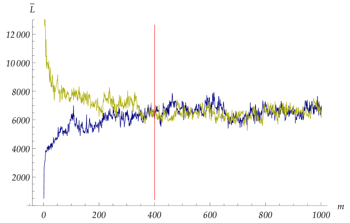
Figure 21: Average defect length $\overline{L}$ in the bulk as a function of the number of measures for a $\mathcal{DLM}(3,4)$ $512\times 1024$ lattice on the $V/H=2$ cylinder. This plot was realized for $n=20$, $m=1000$ and $\Delta=200\times 10^{6}$.

The approximate point of thermalization for $\mathcal{DLM}(3,4)$ on the cylinder of size $H=512$ and $V=1024$ is represented in figure 21 by a vertical line at $m=400$. After that point, the average value fluctuates around $\overline{L}=6500$ which, according to equation (21) with $R=\sqrt{523\,776}\simeq 723.7$, corresponds to $d_{h}^{H\times V}=1.33$. This is to be compared with the final measurement of table 2, $\widehat{d_{h}}^{H\times V}=1.3323\pm 0.0004$. To illustrate the reliability of this thermalization point, we plotted two datasets in figure 21: the dark one corresponds to a set of measures started from a configuration having the smallest possible defect length in the bulk, that is $L=L_{\text{min}}=512$, while the light one corresponds to a set started from the maximal defect length $L=L_{\text{max}}=R^{2}=523\,776$.

B.2 Statistical analysis

We give the details here of the methods used for obtaining confidence intervals on the different measures, on how the linear regressions, or fits, of the data were done, and also what processes were used to discriminate between a good and a bad linear regression. For more details on these subjects, see Draper and Smith [9].

B.2.1 Confidence interval

For an experiment consisting of $n$ independent Markov chains, e.g. $n$ computers or processes, and a total of $m$ measurements $Q_{i,j}$ per chain, where $i$ labels the chain and $j$ the datum, the unbiased estimator of the expected value $\mathrm{\mathbf{E}}[Q]=\overline{Q}$ of an observable $Q$ is given by the grand sample average

$$\widehat{Q}=\frac{1}{n}\sum_{i=1}^{n}\overline{Q}_{i},$$

where $\overline{Q}_{i}=\frac{1}{m}\sum_{j=1}^{m}Q_{i,j}$ is the average value of the $i$-th Markov chain. To obtain a confidence interval on $\widehat{Q}$, we first need to compute the unbiased sample variance

$$\widehat{\sigma}^{2}=\frac{1}{n-1}\sum_{i=1}^{n}\left(\overline{Q}_{i}-\widehat{Q}\right)^{2}.$$

In this work, some of the observables $d_{S}^{H\times V}$ were measured with a small number $n$ of Markov chains ($n\sim 20$). In these cases, it is better to replace the approximate $95\%$ confidence interval $2\widehat{\sigma}/\sqrt{n}$ by the correct

$$\left[\widehat{Q}-\tau_{n-1}(0.95)\frac{\widehat{\sigma}}{\sqrt{n}},\;\widehat{Q}+\tau_{n-1}(0.95)\frac{\widehat{\sigma}}{\sqrt{n}}\right],$$ (31)

where $\tau_{n-1}$ is the inverse Student t-distribution with $n-1$ degrees of freedom. For $n=20$ observations, the factor $\tau_{19}$ of equation (31) equals approximately $2.093$.

B.2.2 Linear regression

The estimated fractal dimension of the different observables in the continuum scaling limit, as $R\rightarrow\infty$ in (21), is obtained by extrapolating the linear regression of the measurement data acquired at finite $R$’s. For an experiment of $n_{1}+n_{2}+\dotsb+n_{\ell}\equiv n$ total measures (sample points) of the observable, with $n_{i}$ the number of measures for the $i$-th lattice size (e.g. $H_{i}=32,H_{i+1}=64$, etc.), the most general linear model with $p$ parameters is:

$$Y_{i}=\beta_{0}+\beta_{1}X_{i1}+\beta_{2}X_{i2}+\dotsb+\beta_{(p-1)}X_{i(p-1)}+\epsilon_{i},$$ (32)

where $Y_{i}$, $i=1,2,\dotsc,n$, are the sample points, $\beta_{k}$, $k=0,1,\dotsc,p-1$, are parameters associated with the $p$ independent variables $X_{ik}$, and $\epsilon_{i}\sim N\left(0,\sigma_{i}^{2}\right)$ is the $i$-th random error associated with $Y_{i}$. We shall be interested in polynomial fits, for which $X_{ij}=X_{i}^{j}$, with $X_{i}=1/\ln R(H_{i},V_{i})$. Moreover, $Y_{i}$ corresponds to the measured fractal dimension $d_{S}^{H_{i}\times V_{i}}$ at $R(H_{i},V_{i})$. The equation (32) can be rewritten in matrix notation as

$$\mathbf{Y}=X\boldsymbol{\beta}+\boldsymbol{\epsilon},$$ (33)

where $\mathbf{Y}$ and $\boldsymbol{\epsilon}$ are $n\times 1$ vectors, $\boldsymbol{\beta}$ is a $p\times 1$ vector, and $X$ is a $n\times p$ matrix. Note that the first column of $X$, related to $\beta_{0}$, is filled with $1$’s. The fitted equation,

$$\widehat{\mathbf{Y}}=X\boldsymbol{\widehat{\beta}},$$ (34)

is such that $\widehat{\mathbf{Y}}=\mathrm{\mathbf{E}}[\mathbf{Y}]$ and $\boldsymbol{\widehat{\beta}}=\mathrm{\mathbf{E}}[\boldsymbol{\beta}]$ are unbiased estimators of $\mathbf{Y}$ and $\boldsymbol{\beta}$, respectively; these are the quantities we need to evaluate.

The difficulty with the present datasets is that the observables $d_{S}^{H_{i}\times V_{i}}$ have not been measured with the same precision, that is, their variances depend on the size of the lattice. And when $\mathrm{\mathbf{Var}}[\boldsymbol{\epsilon}]\equiv\sigma^{2}V\neq\sigma^{2}\mathds{1}_{n}$, with $\sigma^{2}V_{ij}=\mathrm{\mathbf{Cov}}[\epsilon_{i},\epsilon_{j}]$ and $\sigma$ a positive constant, one cannot rely on ordinary least squares (OLS) for obtaining an unbiased linear regression, but must count instead on weighted least squares (WLS). In other words, if the sample variances $\sigma^{2}V_{ii}=\mathrm{\mathbf{Var}}[\epsilon_{i}]=\mathrm{\mathbf{Var}}[Y_{i}]$ in (32) cannot be considered constant throughout the dataset, one cannot use OLS. Moreover, the WLS method may be used only if $V$ is diagonal, i.e. if the different $\epsilon_{i}$ are uncorrelated. Fortunately, this is the case here as our Markov chains are independent.

The idea behind WLS is to multiply both sides of equation (33) by the constant $n\times n$ matrix $P=V^{-1/2}$, in such a way that the variance of the transformed error $P\boldsymbol{\epsilon}$ becomes constant amongst the dataset; indeed, $\mathrm{\mathbf{Var}}[P\boldsymbol{\epsilon}]=\sigma^{2}\mathds{1}_{n}$ since $P$ is symmetric. In practice, one may set $\sigma^{2}=1$ since this constant is the desired variance of the transformed variable $P\mathbf{Y}$, in which case $V=\mathrm{diag}\bigl{\{}\widehat{\sigma_{1}}^{2},\widehat{\sigma_{2}}^{2},\dotsc,\widehat{\sigma_{n}}^{2}\bigr{\}}$. The expressions for $\boldsymbol{\widehat{\beta}}$, $\mathrm{\mathbf{Var}}\bigl{[}\boldsymbol{\widehat{\beta}}\bigr{]}$ and $\mathrm{\mathbf{Var}}\bigl{[}\widehat{\mathbf{Y}}\bigr{]}$ in the WLS method are obtained by replacing $X$ with $PX$ and $\mathbf{Y}$ with $P\mathbf{Y}$ in the usual OLS expressions. The WLS expressions are then

$$\begin{split}\boldsymbol{\widehat{\beta}}&=\left(X^{\intercal}V^{-1}X\right)^{-1}X^{\intercal}V^{-1}\mathbf{Y}\\ \mathrm{\mathbf{Var}}\bigl{[}\boldsymbol{\widehat{\beta}}\bigr{]}&=\sigma^{2}\left(X^{\intercal}V^{-1}X\right)^{-1}\\ \mathrm{\mathbf{Var}}\bigl{[}\widehat{\mathbf{Y}}\bigr{]}&=\sigma^{2}X\,\mathrm{\mathbf{Var}}\bigl{[}\boldsymbol{\widehat{\beta}}\bigr{]}X^{\intercal}.\end{split}$$ (35)

Since we are interested in polynomial models, the last expression of (35) may be rewritten to yield $\mathrm{\mathbf{Var}}\bigl{[}\widehat{\mathbf{Y}}\bigr{]}$ as a function of $x$:

$$\mathrm{\mathbf{Var}}\bigl{[}\widehat{Y}_{x}\bigr{]} =\sigma^{2}\mathbf{x}^{\intercal}\mathrm{\mathbf{Var}}\bigl{[}\boldsymbol{\widehat{\beta}}\bigr{]}\mathbf{x}$$

$$=\sigma^{2}\left(1,x,x^{2},\dotsc,x^{p-1}\right)\mathrm{\mathbf{Var}}\bigl{[}\boldsymbol{\widehat{\beta}}\bigr{]}\left(1,x,x^{2},\dotsc,x^{p-1}\right)^{\intercal}\equiv E(x),$$ (36)

where $\widehat{Y}_{x}=\mathbf{x}^{\intercal}\widehat{\boldsymbol{\beta}}$ is the linear regression. Using (B.2.2), the $95\%$ confidence limits of $\widehat{Y}_{x}$ as a function of $x$ is

$$\left[\widehat{Y}_{x}-\tau_{n-p}(0.95)E(x),\,\widehat{Y}_{x}+\tau_{n-p}(0.95)E(x)\right],$$ (37)

with $\tau_{n-p}(0.95)$ as in (31).

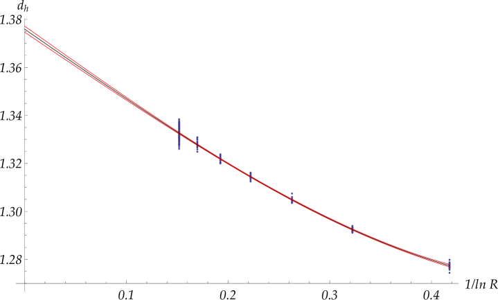
Figure 22: The sample points, the linear regression and its $95\%$ confidence limits for $d_{h}$ of $\mathcal{DLM}(3,4)$ on the $V/H=2$ cylinder.

In figure 22, the results of fitting the model $Y_{i}=\beta_{0}+\beta_{1}X_{i}+\beta_{3}X_{i}^{3}$ to the dataset of the observable $d_{h}$ (eq. (16)) for $\mathcal{DLM}(3,4)$ on the $V/H=2$ cylinder are shown. The average of $d_{h}$ for each run at each size $H\times V$ is shown by a small dot. The bottom and top curves are the confidence limits obtained by (37), and the central curve corresponds to the fit $\widehat{Y}_{x}$. The $95\%$ confidence interval at $1/lnR=0$ is $[1.3744,1.3770]$, thus $\widehat{d_{h}}=1.3757\pm 0.0013$ (cf table 3).

B.2.3 Model testing

Once a linear regression has been obtained, it is necessary to attest its validity and quality. To do this, the popular Pearson correlation coefficient $\left.\sum_{i=1}^{n}\bigl{(}\widehat{Y}_{i}-\overline{Y}\bigr{)}^{2}\right/\sum_{i=1}^{n}\bigl{(}Y_{i}-\overline{Y}\bigr{)}^{2}$ can be of help, but alone may lead to biased results, as discussed in § 11.2 of Draper and Smith [9], especially if an extrapolation from the fit is intended. To complement the correlation coefficient, one may use the $F$-test that compares different models of linear regression for $\mathbf{Y}$. To do so, we must first fix the full model that contains all the $\beta$ parameters that are sensible to use. For instance, our linear regressions used a polynomial model of order 3. Higher order polynomials would have required data on more lattice sizes. The full model is thus

$$Y_{i}=\beta_{0}+\beta_{1}X_{i}+\beta_{2}X_{i}^{2}+\beta_{3}X_{i}^{3}+\epsilon_{i}.$$ (38)

Different models are then compared with the full model. The $F$-test is used to verify linear hypotheses. For example, we may want to compare the quality of the fit obtained, say for a cubic model like (38) but with $\beta_{2}=0$, or an even model where $\beta_{1}=\beta_{3}=0$. We might also want to test a hypothesis of the form $\beta_{0}+2\beta_{1}=4$ and $\beta_{0}+\beta_{1}+\beta_{3}=-1$, where there are now two relations to be satisfied at the same time. More generally, a linear hypothesis can be written as

$$H_{0}:R\boldsymbol{\beta}=\mathbf{r},$$ (39)

where $R$ is an $m\times p$ matrix providing $m$ linear relations amongst the $\beta$’s, where $q$ of these restrictions are linearly independent. The $m\times 1$ vector $\mathbf{r}$ contains the constants of the $m$ relations.

To verify such a hypothesis, both the estimator $\widehat{\boldsymbol{\beta_{r}}}$ of the restricted model, $\mathbf{Y}=X\boldsymbol{\beta_{r}}+\boldsymbol{\epsilon}$,

$$\widehat{\boldsymbol{\beta_{r}}}=\widehat{\boldsymbol{\beta}}+\bigl{(}X^{\intercal}V^{-1}X\bigr{)}^{-1}R^{\intercal}\Bigl{[}R\bigl{(}X^{\intercal}V^{-1}X\bigr{)}^{-1}R^{\intercal}\Bigr{]}^{-1}\bigl{(}\mathbf{r}-R\widehat{\boldsymbol{\beta}}\bigr{)},$$ (40)

and the estimator $\widehat{\boldsymbol{\beta}}$ of the full model are computed. Then the residual sum of squares $\mathrm{SSE}\bigl{(}\widehat{\boldsymbol{\beta_{r}}}\bigr{)}$ and $\mathrm{SSE}\bigl{(}\widehat{\boldsymbol{\beta}}\bigr{)}$ for both models are obtained. Their estimators are defined by

$$\mathrm{SSE}\bigl{(}\widehat{\boldsymbol{\beta}}\bigr{)}=\bigl{(}\mathbf{Y}-X\widehat{\boldsymbol{\beta}}\bigr{)}^{\intercal}\bigl{(}\mathbf{Y}-X\widehat{\boldsymbol{\beta}}\bigr{)},$$ (41)

and similarly for $\widehat{\boldsymbol{\beta_{r}}}$. Finally, the $F$-test for the hypothesis (39) consists in comparing the ratio

$$f_{H_{0}}=\left(\frac{\mathrm{SSE}\bigl{(}\widehat{\boldsymbol{\beta_{r}}}\bigr{)}-\mathrm{SSE}\bigl{(}\widehat{\boldsymbol{\beta}}\bigr{)}}{\mathrm{SSE}\bigl{(}\widehat{\boldsymbol{\beta}}\bigr{)}}\right)\left(\frac{n-p}{q}\right),$$ (42)

with the value $z$ for which $\int_{0}^{z}F(q,n-p,x)\,\mathrm{d}x=\lambda$, where $\lambda\in[0,1]$ (we chose $\lambda=0.95$ in this work) and the $F$-distribution is

$$F(n_{1},n_{2},x)=\frac{1}{\mathrm{B}\left(\frac{n_{1}}{2},\frac{n_{2}}{2}\right)}\left(\frac{n_{1}}{n_{2}}\right)^{n_{1}/2}x^{\frac{n_{1}}{2}-1}\left(1+\frac{n_{1}}{n_{2}}x\right)^{-(n_{1}+n_{2})/2},$$ (43)

with $\mathrm{B}(x,y)$ the Beta function. Now, if $f_{H_{0}}\leq z$ then, with probability $\lambda$, the dataset does not provide sufficient proof that $H_{0}$ has to be rejected. On the other hand, if $f_{H_{0}}>z$, then the dataset shows that the hypothesis $H_{0}$ is implausible and should be rejected. Different scores coming from different hypotheses concerning the same full model may be compared with each other, the lowest score being the most plausible. We use this test to check whether one or more of the coefficients $\beta_{i}$ could be set to zero. When this is a possibility, we note that the estimated fractal dimension obtained from the restricted model is, most of the time, closer to the theoretical value than that of the full one, and its confidence interval is also smaller. For the dataset of the $d_{h}^{H\times V}$ of $\mathcal{DLM}(3,4)$, the full cubic model of (38) gives $\widehat{d_{h}}=1.377\pm 0.007$, while it is $1.3757\pm 0.0013$ for the restricted model having the lowest score, that is the one with $\beta_{2}=0$.

Appendix C Logarithmic minimal models

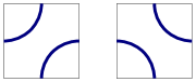
Figure 23: The two equally weighted faces of $\mathcal{LM}$.

Here the lattice models used by Pearce et al. [20] to define the logarithmic minimal models $\mathcal{LM}(p,p^{\prime})$ are recalled. They were used in [23] for simulations of the dense models. The underlying loop gas is based on two elementary faces, illustrated in figure 23. At the isotropic point, the two faces are given an equal weight $\rho_{1}=\rho_{2}$ which can be fixed to $1$. The partition function of the loop gas is then

$$Z=\sum_{\mathcal{L}}\beta^{N},$$ (44)

where $\mathcal{L}$ is the set of all possible loop configurations, $\beta$ the loop fugacity, and $N$ the number of loops in a given configuration. These models do not correspond to a particular solution of the $\mathcal{DLM}$ models ((6) and (2.1.2)) as no value of $\lambda\in[-\pi/2,\pi/2]$ in any of the critical regimes found in Blöte and Nienhuis [5] yields $u=v=0$, $w\neq 0$ and no empty face. The simulations in [23] were done on a cylinder. The boundary conditions consisted in half-circles added at the extremities of the cylinder, as shown in figure 24. Note that, with these boundary conditions, there are $|\mathcal{L}|=2^{H\times V}$ possible configurations.

Figure 24: An example of an $8\times 8$ configuration on the cylinder.

It is these lattice models whose continuum scaling limit was given the name of logarithmic minimal models $\mathcal{LM}(p,p^{\prime})$. Their loop fugacity is given by $\beta=-2cos\left(\frac{\pi}{\bar{\kappa}}\right)$ with $\bar{\kappa}=p^{\prime}/p$ and they are believed to be described by logarithmic CFTs whose central charge and conformal weights are given by (9) and (10).

References

- Aharony and Asikainen [2003] A. Aharony and J. Asikainen. Fractal dimensions and corrections to scaling for critical Potts clusters. Fractals, 11:3–7, 2003, arXiv:cond-mat/0206367.
- Arguin [2002] L.-P. Arguin. Homology of Fortuin-Kasteleyn clusters of Potts models on the torus. J. Stat. Phys., 109:301--310, 2002, arXiv:hep-th/0111193.
- Asikainen et al. [2003] J. Asikainen, A. Aharony, B. B. Mandelbrot, E. M. Rauch, and J. P. Hovi. Fractal geometry of critical Potts clusters. Eur. Phys. Jour. B., 34:479--487, 2003, arXiv:cond-mat/0212216.
- Beffara [2008] V. Beffara. The dimension of the SLE curves. Ann. Probab, 36(4):1421--1452, 2008, arXiv:math/0211322v3 [math.PR].
- Blöte and Nienhuis [1989] H. W. J. Blöte and B. Nienhuis. Critical behaviour and conformal anomaly of the model on the square lattice. J. Phys. A: Math. Gen., 22:1415--1438, 1989.
- Camia and Newman [2006] F. Camia and C. M. Newman. Two-dimensional critical percolation: the full scaling limit. Commun. Math. Phys., 268:1--38, 2006, arXiv:math/0605035v1 [math.PR].
- Chayes and Machta [1998] L. Chayes and J. Machta. Graphical representations and cluster algorithms II. Physica A, 254:477--516, 1998.
- Deng et al. [2007] Y. Deng, T. M. Garoni, W. Guo, H. W. J. Blöte, and A. D. Sokal. Cluster simulations of loop models on two-dimensional lattices. Phys. Rev. Lett., 98:120601, 2007, arXiv:cond-mat/0608447v3 [cond-mat.stat-mech].
- Draper and Smith [1998] N. R. Draper and H. Smith. Applied Regression Analysis. New York, 3rd edition, 1998.
- Dubail et al. [2010] J. Dubail, J. L. Jacobsen, and H. Saleur. Conformal boundary conditions in the critical model and dilute loop models. Nucl. Phys. B, 827:457--502, 2010, arXiv:0905.1382v1.
- Duplantier [1987] B. Duplantier. Critical exponents of Manhattan Hamiltonian walks in two dimensions, from Potts and models. J. Stat. Phys., 49:411--431, 1987.
- Duplantier [1989] B. Duplantier. Two-dimensional fractal geometry, critical phenomena and conformal invariance. Phys. Rep., 184(2–4):229--257, 1989.
- Duplantier [2000] B. Duplantier. Conformally invariant fractals and potential theory. Phys. Rev. Lett., 84(7):1363--1367, 2000.
- Fishman [2006] G. S. Fishman. A First Course in Monte Carlo. Belmont, 2006.
- Grossman and Aharony [1986] T. Grossman and A. Aharony. Structure and perimeters of percolation clusters. J. Phys. A: Math. Gen., 19:L745--L751, 1986.
- Kager and Nienhuis [2004] W. Kager and B. Nienhuis. A guide to stochastic Loewner evolution and its applications. J. Stat. Phys., 115:1149--1229, 2004, arXiv:math-ph/0312056v3.
- Langlands et al. [2000] R. Langlands, M.-A. Lewis, and Y. Saint-Aubin. Universality and conformal invariance for the Ising model in domains with boundary. J. Stat. Phys., 98:131--244, 2000.
- Mandelbrot [1990] B. B. Mandelbrot. Negative fractal dimensions and multifractals. Physica A, 163:306--315, 1990.
- Nienhuis [1990] B. Nienhuis. Critical and multicritical models. Physica A, 163:152--157, 1990.
- Pearce et al. [2006] P. A. Pearce, J. Rasmussen, and J.-B. Zuber. Logarithmic minimal models. J. Stat. Mech., P11017, 2006, arXiv:hep-th/0607232v3.
- Pinson [1994] T. H. Pinson. Critical percolation on the torus. J. Stat. Phys., 75:1167--1177, 1994.
- Rohde and Schramm [2005] S. Rohde and O. Schramm. Basic properties of SLE. Ann. Math., 161:883--924, 2005, arXiv:math/0106036v4 [math.PR].
- Saint-Aubin et al. [2009] Y. Saint-Aubin, P. A. Pearce, and J. Rasmussen. Geometric exponents, SLE and logarithmic minimal models. J. Stat. Mech., P02028, 2009, arXiv:0809.4806v2.
- Saleur and Duplantier [1987] H. Saleur and B. Duplantier. Exact determination of the percolation hull exponent in two dimensions. Phys. Rev. Lett., 58:2325--2328, 1987.
- Sheffield [2006] S. Sheffield. Exploration trees and conformal loop ensembles. Duke Math. J., 147(1):79--129, 2006, arXiv:math/0609167v2 [math.PR].
- Stanley [1977] H. E. Stanley. Cluster shapes at the percolation threshold: an effective cluster dimensionality and its connection with critical-point exponents. J. Phys. A: Math. Gen., 10:L211--L220, 1977.
- Swendsen and Wang [1987] R. H. Swendsen and J.-S. Wang. Nonuniversal critical dynamics in Monte Carlo simulations. Phys. Rev. Lett., 58(2):86--88, 1987.
- Werner [2008] W. Werner. The conformally invariant measure on self-avoiding loops. J. Amer. Math. Soc., 21:137--169, 2008, arXiv:math/0511605v3 [math.PR].