Mathematical Analysis of the BIBEE Approximation for Molecular Solvation: Exact Results for Spherical Inclusions

Abstract

We analyze the mathematically rigorous BIBEE (boundary-integral based electrostatics estimation) approximation of the mixed-dielectric continuum model of molecular electrostatics, using the analytically solvable case of a spherical solute containing an arbitrary charge distribution. Our analysis, which builds on Kirkwood’s solution using spherical harmonics, clarifies important aspects of the approximation and its relationship to Generalized Born models. First, our results suggest a new perspective for analyzing fast electrostatic models: the separation of variables between material properties (the dielectric constants) and geometry (the solute dielectric boundary and charge distribution). Second, we find that the eigenfunctions of the reaction-potential operator are exactly preserved in the BIBEE model for the sphere, which supports the use of this approximation for analyzing charge-charge interactions in molecular binding. Third, a comparison of BIBEE to the recent GB$\epsilon$ theory suggests a modified BIBEE model capable of predicting electrostatic solvation free energies to within 4% of a full numerical Poisson calculation. This modified model leads to a projection-framework understanding of BIBEE and suggests opportunities for future improvements.

1 Introduction

The strong influence of aqueous ionic solvent on biomolecular structure and function necessitates its inclusion in almost all theoretical studies in molecular biophysics [32, 62, 66, 56], but for many applications, including drug screening [36] and protein design [26, 64], explicit-solvent MD [11, 15, 46] remains too expensive. Implicit-solvent models[52, 18, 60, 3] offer a computationally efficient alternative by approximating the solvent influence using a potential of mean force (PMF) approach. The most popular models for the electrostatic component of this PMF are continuum theories based on the Poisson or Poisson–Boltzmann partial differential equations (PDEs) [32, 62, 67, 49, 29]. For all but the simplest molecular models, one must solve the PDE model numerically, which requires substantial computational effort regardless of whether one employs finite-difference methods [67, 24, 33, 23, 43, 70, 16, 12], finite-element methods [69, 17, 4], or the boundary-element methods (BEM) based on boundary-integral equation (BIE) reformulations of the PDE [40, 57, 71, 68, 31, 65, 72, 47, 27, 35, 13, 38, 37, 9, 10, 1, 2]. The discrepancy between this computational effort, which calculates the free energy due to solvent polarization, and the time to required the other energies associated with a particular state (e.g., van der Waals interactions) has motivated significant research towards developing rapidly computed mathematical models that closely reproduce the free-energy landscape of the Poisson equation.

Many of these fast models are designed to be integrated directly into implicit-solvent MD, making differentiability of the energy function a feature of crucial importance. The generalized Born (GB) model  [61, 48, 22, 19, 44, 7, 45, 25, 39, 51, 59, 58, 63, 41, 42] is the most popular, but there are numerous others, notably the ACE model of Schaefer and Karplus [55]. These approaches introduce certain empirical parameters and analytical formulae, such as effective Born radii in GB models, where the approximations rely on physical insights into biomolecular electrostatics problems, including the charge distributions, the dielectric constants, and the near-spherical geometry of many globular proteins [59]. The ability of such models to capture broad features of the energy landscape has led to numerous model refinements, parameterizations, and implementations, but questions remain regarding these empirical models’ generality.

Such models contrast with the BIBEE approximate model we analyze in this paper. The BIBEE (boundary-integral based electrostatics estimation) model derives from a systematic approximation of a well-known BIE formulation of the mixed-dielectric Poisson problem [5, 6], and represents a complementary strategy to obtain an implicit-solvent model: a rigorous operator approximation of the Poisson problem. Important advantages accrue by directly approximating the underlying operator problem rather than exploiting specific features of biomolecular electrostatic problems. For example, the approximation can be analyzed mathematically rather than empirically: we have shown that two variants of BIBEE offer provable upper and lower bounds to the true Poisson solvation free energy [6]. Furthermore, there exists the possibility of developing equally rigorous improvements to the approximation scheme. The results in this paper demonstrate both of these advantages and progress towards an accurate, mathematically sound approximation scheme; however, it must be acknowledged that the model and implementation are not yet suitable for widespread adoption and application in MD. The approach must first overcome substantial challenges before it can be applied to dynamical simulations in which the dielectric boundary changes at each time step (a hurdle that has been surmounted only by a few developers of advanced finite-difference methods, and not yet using boundary-integral approaches). In addition, an naive, unoptimized implementation of BIBEE has been shown to be three to ten times slower than a comparably unoptimized GB implementation[5], a performance discrepancy of some importance as the community pursues ever-longer dynamics simulations.

Here, we study the BIBEE model in the context of the analytically solvable case of a spherical solute. Using this model problem, we highlight an interesting feature of most fast approximate electrostatic models which has been studied in recent GB work and reviews [59], but apparently never articulated explicitly: most, but not all, fast methods assume that the solvation free energy can be calculated using a separation of variables between the problem geometry (here, the charge locations and dielectric boundary) and the material properties, i.e., the dielectric constants. This feature may have implications for the design of improved implicit solvent models or perhaps in other domains. Although to our knowledge the separability approximation has not been discussed directly in the extensive GB literature [7, 3, 20], it is noteworthy that two of the most recent and accurate GB methods, the GBMV (Generalized Born with Molecular Volume) model [34] and the modified GB$\epsilon$ of Sigalov and Onufriev et al. [59], do incorporate corrections that explicitly account for the errors inherent to the separability approximation. The latter work, in particular, provides the basis for high accuracy over a wide range of solute and solvent dielectric constants. Furthermore, a recent review article highlights the material-dependent corrections [20].

Analysis in spherical harmonics allows a straightforward proof that for a sphere, the BIBEE approximation exactly preserves the eigenfunctions of the Poisson reaction-potential operator. The operator eigenfunctions represent charge distributions that do not interact via solvent polarization, and therefore a fast electrostatic model should at least roughly capture eigenfunctions. The sphere geometry also permits a straightforward but detailed comparison of BIBEE and the recently described GB$\epsilon$ model of Sigalov et al., which is based on the most theoretically rigorous analysis of the GB theory of which we are aware. The mathematical insights employed in deriving GB$\epsilon$ leads directly to two improved BIBEE variants: one represents an new and tighter effective lower bound, and another, much more accurate, version is based on the central approximation in the GB$\epsilon$ model. This accurate BIBEE variant relies on a single fitting parameter and provides electrostatic solvation free energies within a few percent of numerical calculations.

The paper is organized as follows: the following section briefly describes the Poisson electrostatic model under consideration, Kirkwood’s spherical-harmonics approach to deriving an closed-form solution to the model [32], and the BIBEE and GB$\epsilon$ approximations. Section 3 details how a separability approach underlies most fast electrostatic schemes. In Section 4, we employ the spherical harmonic analysis to prove the BIBEE and continuum reaction-potential operators share eigenfunctions. In Section 5 we develop improved BIBEE models using the GB$\epsilon$ analysis as a guide. Section 6 concludes the paper with a discussion of implications, possible generalizations, and directions for future work.

2 Theory

2.1 Mixed-Dielectric Poisson Model and Boundary-Integral-Equation Formulation

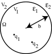
Figure 1: A diagram of the mixed-dielectric Poisson model, showing two discrete point charges in the solute.

A diagram of our model is shown in Fig. 1. The solute, labeled $V_{1}$, is a spherical cavity of radius $b$ with boundary $\Omega$ and dielectric constant $\epsilon_{1}$. The spherical solute is embedded in an infinite homogeneous region, labeled $V_{2}$, with dielectric constant $\epsilon_{2}$. We assume without loss of generality that the solute charge distribution consists of a set of $Q$ point charges $\{q_{k}\}$ at locations ${\bf r}_{k}$. The electrostatic potential in $V_{1}$ satisfies

$$\nabla^{2}\Phi_{1}({\bf r})=-\frac{1}{\epsilon_{1}}\sum_{i=1}^{Q}q_{k}\delta({\bf r}-{\bf r}_{k})$$ (1)

and the potential in $V_{2}$ satisfies the Laplace equation $\nabla^{2}\Phi_{2}({\bf r})=0$. Across the boundary, the potential is continuous and so is the normal component of the displacement field:

$$\Phi_{1}|_{r=b} =\Phi_{2}|_{r=b}$$ (2)

$$\epsilon_{1}\frac{\partial\Phi_{1}}{\partial r}|_{r=b} =\epsilon_{2}\frac{\partial\Phi_{2}}{\partial r}|_{r=b}$$ (3)

where we have defined the normal direction pointing from $V_{1}$ into the solvent region $V_{2}$. Finally, the potential $V_{2}$ is assumed to go to zero as ${\bf r}\rightarrow\infty$. The jump in dielectric constants in the two regions gives rise to a discontinuity in the polarization charge density as one crosses the dielectric boundary [28, 57, 53, 8]. This surface charge density $\sigma({\bf r})$ satisfies the boundary-integral equation

$$\sigma({\bf r})+\hat{\epsilon}\mathchoice{{\vbox{\hbox{$\textstyle-$}}\kern-4.86108pt}}{{\vbox{\hbox{$\scriptstyle-$}}\kern-3.25pt}}{{\vbox{\hbox{$\scriptscriptstyle-$}}\kern-2.29166pt}}{{\vbox{\hbox{$\scriptscriptstyle-$}}\kern-1.875pt}}\!\int_{\Omega}\frac{\partial}{\partial{\bf n}({\bf r})}\frac{1}{4\pi||{\bf r}-{\bf r}^{\prime}||}\sigma({\bf r}^{\prime})d^{2}{\bf r}^{\prime}=-\hat{\epsilon}\sum_{k=1}^{Q}q_{k}\frac{\partial}{\partial{\bf n}({\bf r})}\frac{1}{4\pi||{\bf r}-{\bf r}_{k}||}$$ (4)

where

$$\hat{\epsilon}=\frac{\epsilon_{1}-\epsilon_{2}}{\frac{1}{2}(\epsilon_{1}+\epsilon_{2})}.$$ (5)

and $\mathchoice{{\vbox{\hbox{$\textstyle-$}}\kern-4.86108pt}}{{\vbox{\hbox{$\scriptstyle-$}}\kern-3.25pt}}{{\vbox{\hbox{$\scriptscriptstyle-$}}\kern-2.29166pt}}{{\vbox{\hbox{$\scriptscriptstyle-$}}\kern-1.875pt}}\!\int$ denotes the Cauchy principal value integral. In operator notation, Eq. (4) may be written

$$\left(\mathcal{I}+\hat{\epsilon}\mathcal{D}^{*}\right)\sigma=Bq$$ (6)

where $q$ is the vector of the fixed charges, $B$ maps $q$ to the right-hand side of Eq. (4), $\mathcal{I}$ is the identity operator, and $\mathcal{D}^{*}$ is the normal electric-field operator. The Coulomb potential induced by $\sigma({\bf r})$,

$$\psi({\bf r})=\int_{\Omega}\sigma({\bf r}^{\prime})\frac{1}{4\pi||{\bf r}-{\bf r}^{\prime}||}d^{2}{\bf r}^{\prime},$$ (7)

is the reaction-field potential, and the electrostatic component of the solvation free energy is

$$\Delta G^{\mathrm{el}}_{solv}=\frac{1}{2}\sum_{k=1}^{Q}\psi({\bf r}_{k})q_{k},$$ (8)

Denoting the Coulomb integral operator of Eq. (7) as $C$, the linear mapping from the charge vector $q$ to the reaction potential $\psi$, known as the reaction-potential operator, is

$$\psi=C\left(\mathcal{I}+\hat{\epsilon}\mathcal{D}^{*}\right)^{-1}Bq$$ (9)

so the electrostatic solvation free energy is the quadratic form

$$\Delta G^{\mathrm{el}}_{solv}=\frac{1}{2}q^{T}C\left(\mathcal{I}+\hat{\epsilon}\mathcal{D}^{*}\right)^{-1}Bq.$$ (10)

2.2 Kirkwood’s Solution

We review Kirkwood’s series solution for our model problem [32]. The potential inside $V_{1}$ is given by

$$\Phi_{1}=\sum^{Q}_{k=1}\frac{q_{k}}{\epsilon_{1}\left|{\bf r}-{\bf r}_{k}\right|}+\psi,$$ (11)

where again $\psi$ is the reaction potential. We expand $\psi$ in the associated Legendre functions, keeping only terms valid within $V_{1}$, as

$$\psi=\sum^{\infty}_{n=0}\sum^{n}_{m=-n}B_{nm}r^{n}P_{n}^{m}(\cos\theta)e^{im\phi}.$$ (12)

The potential in region $V_{2}$ may be similarly expanded, keeping terms valid at infinite ${\bf r}$:

$$\Phi_{2}=\sum^{\infty}_{n=0}\sum^{n}_{m=-n}\frac{C_{nm}}{r^{n+1}}P_{n}^{m}(\cos\theta)e^{im\phi}.$$ (13)

To determine the constants appearing in these expansions, we apply the boundary conditions Eqs. (2) and (3) by relating them to the Coulomb portion of $\Phi_{1}$, using the fact that all charges are contained inside the sphere ($r_{k}<r$), as

$$\sum^{Q}_{k=1}\frac{q_{k}}{\epsilon_{1}\left|{\bf r}-{\bf r}_{k}\right|} = \sum^{Q}_{k=1}\frac{q_{k}}{\epsilon_{1}}4\pi\sum^{\infty}_{n=0}\sum^{n}_{m=-n}\frac{1}{2n+1}\frac{r^{n}_{k}}{r^{n+1}}{Y_{n}^{m}}^{*}(\theta_{k},\phi_{k})Y_{n}^{m}(\theta,\phi)$$ (14)

$$= \sum^{Q}_{k=1}\frac{q_{k}}{\epsilon_{1}}4\pi\sum^{\infty}_{n=0}\sum^{n}_{m=-n}\frac{1}{2n+1}\frac{r^{n}_{k}}{r^{n+1}}\sqrt{\frac{2n+1}{4\pi}\frac{(n-|m|)!}{(n+|m|)!}}$$ (16)

$$P_{n}^{m}(\cos\theta_{k})e^{-im\phi_{k}}\sqrt{\frac{2n+1}{4\pi}\frac{(n-|m|)!}{(n+|m|)!}}P_{n}^{m}(\cos\theta)e^{im\phi}$$

$$= \sum^{\infty}_{n=0}\sum^{n}_{m=-n}\frac{E_{nm}}{\epsilon_{1}r^{n+1}}P_{n}^{m}(\cos\theta)e^{im\phi},$$ (17)

where

$$E_{nm}=\sum^{Q}_{k=1}q_{k}r^{n}_{k}\frac{(n-|m|)!}{(n+|m|)!}P_{n}^{m}(\cos\theta_{k})e^{-im\phi_{k}}.$$ (18)

Now the first boundary condition, Eq. (2), gives us the relation

$$\frac{E_{nm}}{\epsilon_{1}}+b^{2n+1}B_{nm}=C_{nm}$$ (19)

where we have equated each $(n,m)$ term in order for the it to hold for all angles. In order to apply Eq. (3), we differentiate each series term by term and equate them,

$$\frac{1}{\epsilon_{2}}E_{nm}-\frac{\epsilon_{1}}{\epsilon_{2}}\frac{n}{n+1}b^{2n+1}B_{nm}=C_{nm}.$$ (20)

We can eliminate the $C_{nm}$ coefficients, to give the reaction field coefficients $B_{nm}$ in terms of the known source charge coefficients $E_{nm}$,

$$B_{nm}=\frac{1}{\epsilon_{1}b^{2n+1}}\frac{(\epsilon_{1}-\epsilon_{2})(n+1)}{\epsilon_{1}n+\epsilon_{2}(n+1)}E_{nm}.$$ (21)

2.3 BIBEE Approximations

The BIBEE/CFA approximation replaces the boundary-integral operator of Eq. (4) with a scaled version of the identity operator, where the scale factor is taken to be $-1/2$, which is the extremal eigenvalue of the boundary-integral operator: thus we have

$$\left(1-\frac{1}{2}\hat{\epsilon}\right)\sigma^{\mathrm{CFA}}=Bq.$$ (22)

This eigenvalue is associated with the constant electric field at the boundary [5], and is the reason that the CFA is exact for a sphere with central charge; the CFA is actually exact for any charge distribution that generates a constant electric field. After calculating an approximate surface charge distribution, the reaction potential is computed just as if one had solved the actual boundary integral equation of Eq. (4), so that

$$\Delta G^{\mathrm{CFA}}=\frac{1}{2}q^{T}C\left(1-\frac{1}{2}\hat{\epsilon}\right)^{-1}Bq$$ (23)

The use of the extremal eigenvalue enables one to prove that the BIBEE/CFA approximate electrostatic solvation free energy is an upper bound to the actual electrostatic solvation free energy [6]. The BIBEE/P approximation takes the scale factor to be $0$, which is the other extremal eigenvalue for spheres (and prolate spheroids):

$$\sigma^{\mathrm{P}}=Bq.$$ (24)

The resulting approximate solvation free energy is a provable lower bound for such surfaces. Though BIBEE/P is not a rigorous lower bound for all surfaces, including oblate spheroids, tests on hundreds of proteins showed that it never failed to provide an effective lower bound [6].

Note that the approximate surface charge densities are scalar multiples of one another, and thus the corresponding approximate reaction-potential operators share a common eigenbasis.

2.4 Generalized-Born Theory and the GB$\epsilon$ Model

In the Generalized-Born (GB) electrostatic model, one associates with each point charge an empirical parameter called an effective Born radius, which is defined so that a spherical ion of that radius would have the same solvation free energy as the original point charge in the solute (i.e., the Born expression for the solvation energy of a spherical ion). In practice, one calculates the effective Born radii approximately using e.g. the Coulomb-field approximation or extensions thereof. The reaction potential at a charge at ${\bf r}_{i}$ due to a unit charge at ${\bf r}_{j}$, when the two effective radii are $R_{i}$ and $R_{j}$, and the distance between them is $r_{ij}$, is given by

$$\varphi({\bf r}_{i})=-\left(\frac{1}{\epsilon_{1}}-\frac{1}{\epsilon_{2}}\right)\frac{1}{f_{ij}^{\mathrm{GB}}(r_{ij},R_{i},R_{j})}$$ (25)

where $f_{ij}^{\mathrm{GB}}$ is the usual Still equation

$$f_{ij}^{\mathrm{GB}}(r_{ij},R_{i},R_{j})=\sqrt{r_{ij}^{2}+R_{i}R_{j}\exp(-r_{ij}^{2}/4R_{i}R_{j})}.$$ (26)

The model has been demonstrated to exhibit remarkable fidelity to much more expensive numerical solutions of the Poisson equation, but the model’s largely empirical nature poses challenges for extending the model to more general configurations. A substantial recent advance in GB theory was achieved by Sigalov et al., who introduced the GB$\epsilon$ model to provide improved accuracy of GB methods for a wider range of dielectric constants [59], not just in the usual biomolecular case in which $\epsilon_{1}/\epsilon_{2}\ll 1$.

The GB$\epsilon$ model derives from analytically solvable cases of point charges’ self-energies in the limits $\epsilon_{1}/\epsilon_{2}\to\infty$ and $\epsilon_{1}/\epsilon_{2}\to 0$ for a spherical solute. Specifically, for an arbitrary solute, the authors define an electrostatic radius $A$ by computing $\lim_{\epsilon_{1}/\epsilon_{2}\to\infty}\Delta G^{\mathrm{el}}_{ii}=\Delta G_{ii}^{\mathrm{el}}(\epsilon_{1}/\epsilon_{2}\to\infty)$ and then setting $A$ according to

$$\Delta G^{\mathrm{el}}_{ii}(\epsilon_{1}/\epsilon_{2}\to\infty)=-\frac{q_{i}^{2}}{2}\left(\frac{1}{\epsilon_{1}}-\frac{1}{\epsilon_{2}}\right)\frac{1}{A}.$$ (27)

The $i$th charge’s effective Born radius for the limit $\epsilon_{1}/\epsilon_{2}\to 0$ is denoted by $\tilde{R}_{i}$; the slight change of notation denotes the effective Born radius in the limit $\epsilon_{1}/\epsilon_{2}\to 0$, as opposed to the standard definition. These parameters are defined by first computing each charge’s effective distance $r_{i}$ from the center of the molecule via

$$\Delta G_{ii}^{\mathrm{el}}(\epsilon_{1}/\epsilon_{2}\to 0)=-\frac{q_{i}^{2}}{2}\left(\frac{1}{\epsilon_{1}}-\frac{1}{\epsilon_{2}}\right)\frac{1}{A-r_{i}^{2}/A}$$ (28)

and then setting $\tilde{R}_{i}=A-r_{i}^{2}/A$ so as to recover the familiar Born self-energy expression

$$\Delta G_{ii}^{\mathrm{Born}}=-\frac{q_{i}^{2}}{2}\left(\frac{1}{\epsilon_{1}}-\frac{1}{\epsilon_{2}}\right)\frac{1}{\tilde{R}_{i}}$$ (29)

Kirkwood’s exact expression for two charges’ interaction in a sphere of radius $A$ can be expressed succinctly via [59]

$$\Delta G^{\mathrm{el}}_{ij}=-q_{i}q_{j}\frac{1-\epsilon_{1}/\epsilon_{2}}{A\epsilon_{1}}\sum_{l=0}^{\infty}\frac{t_{ij}^{l}P_{l}(\cos\theta)}{1+\frac{l}{l+1}\frac{\epsilon_{1}}{\epsilon_{2}}},$$ (30)

where $t_{ij}=|{\bf r}_{i}||{\bf r}_{j}|/A^{2}$, $P_{l}(x)$ is the Legendre polynomial, and $\theta$ is the angle between the charges with respect to the origin. The GB$\epsilon$ model approximates this expression for arbitrary molecular shapes, given the electrostatic radius $A$ and the effective radii $\tilde{R}_{i}$, as

$$\Delta G^{\mathrm{el}}_{ij}=-\frac{1}{2}\left(\frac{1}{\epsilon_{1}}-\frac{1}{\epsilon_{2}}\right)\frac{q_{i}q_{j}}{1+\alpha\epsilon_{1}/\epsilon_{2}}\left[\frac{1}{f_{ij}^{\mathrm{GB}}(r_{ij},\tilde{R}_{i},\tilde{R}_{j})}+\frac{\alpha\epsilon_{1}/\epsilon_{2}}{A}\right]$$ (31)

and the parameter $\alpha=0.57$ has been determined to minimize the error between this approximation and the analytical result [59].

Three important features of this model should be noted. First, the analysis of the GB$\epsilon$ model provides a mathematically justified rationalization for the functional form of the Still equation, which explains why GB methods enjoy the surprising success. Second, the method still requires the calculation (or estimation) of each charge’s self-energy, albeit in the limit $\epsilon_{1}/\epsilon_{2}\to 0$ rather than for the actual dielectric constants of interest. Third, the parameter $\alpha$ was determined by first expressing the pairwise interaction between charges as a sum over spherical harmonics and then manipulating terms to develop an accurate approximation to the infinite sum.

3 Separability

In both the BIBEE and standard GB approaches, the reaction potential at ${\bf r}_{i}$ due to a +1$e$ charge at ${\bf r}_{j}$ can be written in the general form

$$\psi({\bf r}_{i})=g(\epsilon_{1},\epsilon_{2})h(V_{1},{\bf r}_{i},{\bf r}_{j})$$ (32)

where $g(\epsilon_{1},\epsilon_{2})$ is a function only of the dielectric constants and $h(V_{1},{\bf r}_{i},{\bf r}_{j})$ is a function only of the solute geometry (denoted by the volume) and the charge positions. Thus, both fast electrostatic models employ a separable functional form for the reaction potential. Ample evidence supports that these methods exhibit remarkable properties in capturing the electrostatic free energy of solvation, but surprisingly there exists no clear argument why a separable representation might be accurate: that is, for the Poisson equation nothing in either the partial-differential form

$$\nabla\cdot\left(\epsilon({\bf r})\nabla\varphi({\bf r})\right)=-\rho({\bf r})$$ (33)

or its boundary-integral form would a priori suggest that one could obtain an adequate approximation by moving to a separable representation.

Formally, and specializing the analysis to the sphere case, an off-center charge excites at least one mode for each multipole order; as shown by Sigalov et al., the excitation/response relation for a mode depends on both the multipole order $l$ and the dielectric ratio $\beta=\epsilon_{2}/\epsilon_{1}$ via

$$\frac{1}{1+\beta\frac{l}{l+1}},$$ (34)

and therefore it is not possible to define an exact separable energy function. The many successes of GB theory clearly argue that separable energy functions provide satisfactory accuracy for many applications, and two more arguments can also be made to support their study. First, improvements on the original GB/CFA approach have almost exclusively modified the function $h$, and in particular the formulae associated with calculating the effective Born radii; thus, the observed substantial advances in GB models have virtually all maintained separability as a central mathematical feature. Second, earlier studies of BIBEE illustrated that modern GB methods very accurately capture the eigenvalues of the reaction-potential operator and reproduce the operator eigenvectors only with moderate accuracy; in contrast, BIBEE models provide an excellent approximation to the eigenvectors but only moderate reproduction of the eigenvalues. Because these two drastically different approximations can capture these distinct features with only minor modifications to separability, it seems quite possible that one approximation may be found that captures the best features of both approaches.

In GB theory, deviations from separable response are compensated somewhat by the fact that the radius $R_{i}$ is set so that even if the potential itself is large, the error in $\psi^{\mathrm{GB}}({\bf r}_{i})$ is zero (assuming perfect radii). Because the Still equation is a smooth function designed to approximately capture the distance-dependence of the reaction potential [61], the error will be relatively small nearby as well, i.e. for the closest charges. This interpolatory feature is an extra source of accuracy for GB-type methods in standard situations with $\epsilon_{1}<<\epsilon_{2}$; nevertheless, as pointed out by Onufriev and collaborators, high accuracy is not a general property for all values of these two parameters.

Sigalov et al. presented two key insights that provide a strong theoretical basis for designing accurate and rapidly computed, but not separable methods such as their GB$\epsilon$ model. First, the lowest mode $l=0$ is associated with the response due to the solute monopole moment. This mode is distinct because it is associated with a constant potential inside, which is why GB$\epsilon$ makes effective use of the seemingly counterintuitive limit of a conductor solute (i.e. $\epsilon_{1}\to\infty$): a conductor has a constant potential inside it. Treating this mode distinctly, as GB$\epsilon$ does, offers certain advantages and we return to this idea later to improve BIBEE.

The next crucial insight in the GB$\epsilon$ model is that by separating the $l=0$ term, it becomes much more reasonable to capture a reasonable approximation to the relationship between the dielectric constants and the ratio $l/(l+1)$. For the higher order terms $l=1,2,\ldots$, the mode/dielectric ratio coupling terms are all between $\frac{1}{2}\beta$ and $\beta$, and the highest frequency modes generally exert a very small influence on the total energetics. In constructing the GB$\epsilon$ model, the authors minimized the error in the solute reaction potential and found that $\frac{l}{l+1}\approx 0.57$ (this is the parameter $\alpha$) sufficed to give excellent accuracy with a purely separable representation. This value lies between the dipole and quadrupole terms ($l=1$ and $l=2$).

4 Analysis of BIBEE for a Spherical Solute

The continuity of the normal dielectric displacement can also be interpreted as the accumulation of a single-layer surface charge $\sigma$,

$$\sigma = \left[E_{\perp}\right]$$ (35)

$$= \frac{\partial\Phi_{2}}{\partial r}-\frac{\partial\Phi_{1}}{\partial r}$$ (36)

$$= \frac{\epsilon_{1}}{\epsilon_{2}}\frac{\partial\Phi_{1}}{\partial r}-\frac{\partial\Phi_{1}}{\partial r}$$ (37)

$$= \frac{\epsilon_{1}-\epsilon_{2}}{\epsilon_{2}}\frac{\partial\Phi_{1}}{\partial r}$$ (38)

where the third line makes use of Eq. (3). In the original formulation of the BIBEE approximation, we replace the integral operator mapping the normal electric field at the surface to a charge density with a diagonal approximation [5]. However, one may alternatively consider this approximation as a deformation of the above boundary condition to the requirement that the induced surface charges be proportional to the Coulomb Field Approximation (CFA), i.e. neglecting the reaction-field component:

$$\sigma^{CFA}=\frac{\epsilon_{1}-\epsilon_{2}}{\epsilon_{2}}\frac{\partial\Phi^{C}_{1}}{\partial r}$$ (39)

where

$$\Phi^{C}_{1}=\Phi_{1}-\psi=\sum^{Q}_{k=1}\frac{q_{k}}{\epsilon_{1}\left|{\bf r}-{\bf r}_{k}\right|}.$$ (40)

Using Eqs. (39) and (36), we can derive a boundary condition for the BIBEE/CFA approximation

$$\frac{\epsilon_{1}}{\epsilon_{2}}\frac{\partial\Phi^{C}_{1}}{\partial r}=\frac{\partial\Phi_{2}}{\partial r}-\frac{\partial\psi}{\partial r}.$$ (41)

We can now derive a similar relation to Eq. (20) by equating coefficients,

$$\frac{1}{\epsilon_{2}}E_{nm}-\frac{n}{n+1}b^{2n+1}B_{nm}=C_{nm}$$ (42)

which using Eq. (19) gives

$$B^{CFA}_{nm}=\frac{\epsilon_{1}-\epsilon_{2}}{\epsilon_{1}\epsilon_{2}}\frac{n+1}{2n+1}\frac{1}{b^{2n+1}}E_{nm}.$$ (43)

We emphasize that Eq. (43) shows explicitly that the approximation has produced a separated representation in terms of $n$ and $\epsilon$. We can derive a similar expression for the approximate lower bound BIBEE/P given that

$$\sigma^{P}=\frac{\epsilon_{1}-\epsilon_{2}}{\frac{1}{2}(\epsilon_{1}+\epsilon_{2})}\frac{\partial\Phi^{C}_{1}}{\partial r},$$ (44)

which leads to the modified boundary condition

$$\frac{3\epsilon_{1}-\epsilon_{2}}{\epsilon_{1}+\epsilon_{2}}\frac{\partial\Phi^{C}_{1}}{\partial r}=\frac{\partial\Phi_{2}}{\partial r}-\frac{\partial\psi}{\partial r}.$$ (45)

We can now derive a relation analogous to both Eqs. (20) and (42) by equating coefficients,

$$\frac{3\epsilon_{1}-\epsilon_{2}}{\epsilon_{1}(\epsilon_{1}+\epsilon_{2})}E_{nm}-\frac{n}{n+1}b^{2n+1}B_{nm}=C_{nm}$$ (46)

which using Eq. (19) gives

$$B^{P}_{nm}=\frac{2(\epsilon_{1}-\epsilon_{2})}{\epsilon_{1}(\epsilon_{1}+\epsilon_{2})}\frac{n+1}{2n+1}\frac{1}{b^{2n+1}}E_{nm}.$$ (47)

Removing the common factor from Eqs. (21), (43), and (47),

$$\gamma_{nm}=\frac{\epsilon_{1}-\epsilon_{2}}{\epsilon_{1}}(n+1)\frac{1}{b^{2n+1}}E_{nm},$$ (48)

so that

$$B_{nm} = \frac{1}{\epsilon_{1}n+\epsilon_{2}(n+1)}\gamma_{nm}$$ (49)

$$B^{CFA}_{nm} = \frac{1}{\epsilon_{2}}\frac{1}{2n+1}\gamma_{nm}$$ (50)

$$B^{P}_{nm} = \frac{1}{\epsilon_{1}+\epsilon_{2}}\frac{1}{n+\frac{1}{2}}\gamma_{nm}.$$ (51)

Clearly, if $\epsilon_{1}=\epsilon_{2}=\epsilon$, i.e. in a uniform medium with no reaction term $\psi$, then both approximations are exact:

$$B_{nm}=B^{CFA}_{nm}=B^{P}_{nm}=\frac{1}{\epsilon(2n+1)}\gamma_{nm}.$$ (52)

4.1 BIBEE Reaction-Potential Eigenfunctions Are Exact

We can now show that the approximate BIBEE reaction-potential operators have identical eigenspaces to the original operator, by examining the effect on a unit spherical harmonic charge distribution input

$$\hat{\rho}_{n^{\prime}m^{\prime}}=P_{n^{\prime}}^{m^{\prime}}(\cos\hat{\theta})e^{-im^{\prime}\hat{\phi}}.$$ (53)

This source produces a Coulomb potential $\hat{\Phi}^{C}_{1}$ whose expansion is defined by

$$\hat{E}_{nm}=\hat{r}^{n}P_{n}^{m}(\cos\hat{\theta})e^{-im\hat{\phi}}\delta_{nn^{\prime}}\delta_{mm^{\prime}}$$ (54)

where $\delta_{ij}$ is the Kronecker delta. Then, from Eqs. (49)–(51), it is clear that

$$\hat{B}_{nm} = \frac{(\epsilon_{1}-\epsilon_{2})(n+1)}{\epsilon_{1}\left(\epsilon_{1}n+\epsilon_{2}(n+1)\right)}\frac{\hat{r}^{n}}{b^{2n+1}}P_{n}^{m}(\cos\hat{\theta})e^{-im\hat{\phi}}\delta_{nn^{\prime}}\delta_{mm^{\prime}}$$ (55)

$$\hat{B}^{CFA}_{nm} = \frac{(\epsilon_{1}-\epsilon_{2})(n+1)}{\epsilon_{1}\epsilon_{2}(2n+1)}\frac{\hat{r}^{n}}{b^{2n+1}}P_{n}^{m}(\cos\hat{\theta})e^{-im\hat{\phi}}\delta_{nn^{\prime}}\delta_{mm^{\prime}}$$ (56)

$$\hat{B}^{P}_{nm} = \frac{(\epsilon_{1}-\epsilon_{2})(n+1)}{\epsilon_{1}\left(\epsilon_{1}+\epsilon_{2}\right)\left(n+\frac{1}{2}\right)}\frac{\hat{r}^{n}}{b^{2n+1}}P_{n}^{m}(\cos\hat{\theta})e^{-im\hat{\phi}}\delta_{nn^{\prime}}\delta_{mm^{\prime}}$$ (57)

so that each reaction-field has a response only in the input harmonic $(n^{\prime},m^{\prime})$. Therefore each input $\hat{\rho}_{n^{\prime}m^{\prime}}$ is an eigenfunction of the exact reaction-potential operator and also an eigenfunction of the BIBEE operators. Because the spherical harmonics form a complete basis, the eigenspaces are identical.

4.2 Asymptotic Behavior of BIBEE Approximations

Comparing Eqs. (21) with (43), we see that the $n=0$ mode is exact in the BIBEE/CFA approximation,

$$B_{00}=B^{CFA}_{00}=\frac{\gamma_{00}}{\epsilon_{2}},$$ (58)

whereas BIBEE/P approaches the exact response in the limit $n\to\infty$:

$$\lim_{n\to\infty}B_{nm}=\lim_{n\to\infty}B^{P}_{nm}=\frac{1}{(\epsilon_{1}+\epsilon_{2})n}\gamma_{nm}.$$ (59)

In most biomolecule modeling problems, the cavity $V_{1}$ has a very low dielectric constant compared to the surrounding medium $V_{2}$ (i.e. if $\epsilon_{1}\ll\epsilon_{2}$). In the limit $\epsilon_{1}/\epsilon_{2}\to 0$,

$$\lim_{\epsilon_{1}/\epsilon_{2}\to 0}B_{nm} = \frac{\gamma_{nm}}{\epsilon_{2}(n+1)}$$ (60)

$$\lim_{\epsilon_{1}/\epsilon_{2}\to 0}B^{CFA}_{nm} = \frac{\gamma_{nm}}{\epsilon_{2}(2n+1)},$$ (61)

$$\lim_{\epsilon_{1}/\epsilon_{2}\to 0}B^{P}_{nm} = \frac{\gamma_{nm}}{\epsilon_{2}\left(n+\frac{1}{2}\right)},$$ (62)

so that the approximation ratios are

$$\frac{B^{CFA}_{nm}}{B_{nm}} = \frac{n+1}{2n+1},$$ (63)

$$\frac{B^{P}_{nm}}{B_{nm}} = \frac{n+1}{n+\frac{1}{2}}.$$ (64)

We see that BIBEE/CFA is exact in the case of the uniform field, and the modal contribution can be off by a factor of 2 for very high spatial-frequency charge distributions. This mirrors the bounds derived previously [5]. In the case of BIBEE/P, the situation is reversed: the uniform field can be incorrect by a factor of 2, whereas the high frequency field is exact in the limit. Furthermore, it is clear that BIBEE/CFA underestimates coefficients, which is why BIBEE/CFA solvation free energy estimates are rigorous upper bounds for the true solvation free energies (which are negative quantities) [6]. Conversely, BIBEE/P overestimates the coefficients and give lower bounds.

These asymptotic relations can be compared to Grycuk’s analysis [25]. The BIBEE/CFA approximation has an exact monopole moment, corresponding to Grycuk’s case of a charge centered in region $V_{1}$. Likewise, the observed inaccuracies for charges near the cavity surface correspond to higher multipole moments, where we see that BIBEE/CFA overestimates the coefficients by a factor of 2, the same factor found by Grycuk. The BIBEE/P model easily provides an accurate approximation in this limit.

5 Improved BIBEE Models

The considerations in Section 3 suggest a strategy to improve the BIBEE model: one should use the BIBEE/CFA approximation for the monopole moment and a different approximation for the higher-order terms. We explore two approximations here. In the simplest, BIBEE/P is used for the other terms; in the second, we follow the approach in GB$\epsilon$ and use an effective parameter. By using BIBEE/CFA only for the monopole moment, one ensures that the constant component of the reaction potential is captured exactly, just as the GB$\epsilon$ model was designed to do. The strategy is easy to adopt as an improved BIBEE model because it is associated with the constant surface-charge distribution, and therefore the separation is analytically exact.

For the sphere, the reaction potential expansion in this hybrid model is given by $B^{CFA}_{00}$ in combination with $B^{P}_{nm}$ for $n,m\neq 0$. The alternate interpretation, suitable for application to general geometries, is that one calculates an approximate surface charge $\hat{\sigma}$ as a sum of BIBEE/CFA and BIBEE/P components:

$$\hat{\sigma}=\sigma^{\mathrm{CFA,monopole}}+\sigma^{\mathrm{P,other}}.$$ (65)

To obtain these components, one first computes $Bq$ as before, i.e. the Coulomb electric field at the boundary. This field is then decomposed into two terms: its mean value $<Bq>$, and the field minus the mean, $Bq-<Bq>$. One then employs the usual approximations (22) and (24), so that

$$(1-\frac{1}{2}\hat{\epsilon})\sigma^{\mathrm{CFA,monopole}} = <Bq>$$ (66)

$$\sigma^{\mathrm{P,other}} = Bq-<Bq>.$$ (67)

This approach has been validated using a sphere with random charge distributions, and we note that this combination of approximations provides a correction for charged species but gives exactly the BIBEE/P result for net-neutral charge distributions.

Note that the modified BIBEE approach (BIBEE/M) leads to a reaction potential that is not separable in the sense that it may be written in the form of Eq. (32); instead, the potential is the sum of two terms that are themselves separable. Defining the operator $B$ of Eq. (6) via $B=\hat{\epsilon}\tilde{B}$, the BIBEE/M reaction potential is

$$\psi^{M} = C\hat{\sigma}$$ (68)

$$= \hat{\epsilon}C\tilde{B}q+\hat{\epsilon}\left((1-\frac{1}{2}\hat{\epsilon})^{-1}-1\right)C<\tilde{B}q>.$$ (69)

Figure 2(a) shows exact and approximate electrostatic solvation free energies for sets of 25 randomly located point charges in a sphere of radius 5 Å, where the point charges are randomly assigned values less than 0.5 in magnitude; the dielectric constants are taken to be $\epsilon_{1}=4$ and $\epsilon_{2}=80$. As expected, this approach is always a more accurate estimate than BIBEE/P; in fact, because the monopole mode is captured exactly and the others are overestimated when $\lambda=0$, BIBEE/M is a tighter lower bound for the sphere than BIBEE/P. Though the majority of random charge distributions see significantly improved estimates between BIBEE/P and BIBEE/M, contributions from other modes can still strongly affect the overall free energy and lead to little improvement. However, employing the method on 200 proteins from the Feig et al. test set [21] illustrates that the improvement is quite modest at best in practice, as shown in Figure 2(b). These calculations were conducted using CHARMM22 radii and charges [30], $\epsilon_{1}=4$, $\epsilon_{2}=80$, and the molecular surface with probe radius 1.4 Å; triangular discretizations were computed using MSMS [54]. Clearly, despite improvements in accuracy, more improvement is still needed in order to predict solvation free energies with the same accuracy as sophisticated Generalized Born methods.

As shown in Section 4, the BIBEE/P eigenvalue approximation $\lambda=0$ is exact in the limit as the multipole order goes to infinity. An alternative modified BIBEE might employ instead the GB$\epsilon$ strategy of choosing an approximation suitable for the dipole and quadrupole; like BIBEE/M with $\lambda=0$, this strategy also leads to a representation that is the sum of separable terms. For the electric-field operator on the sphere, these eigenvalues are $\lambda=-1/6$ and $\lambda=-1/10$; we therefore tested a range of $\lambda$ from -0.10 to -0.22 on 50 of the proteins from the Feig et al. test set; we used the larger magnitude limits to account for the larger dipole eigenvalues of ellipsoidal geometries [50]. In fact, the simple parameter sweep illustrated that $\lambda=-0.20$ offered approximately the best accuracy (Figure 3), with a root-mean-square-deviation (RMSD) of 18.1 kcal/mol, corresponding to a mean deviation of 3.6%; Table 1 contains the corresponding results for different $\lambda$. Future work should examine the possibility of identifying the molecule’s approximate best-fit ellipsoid, following the recent ALPB model of Sigalov, Onufriev et al. [58]; such an approach might provide a rigorous, parameter-free model as opposed to the one-parameter approach here.

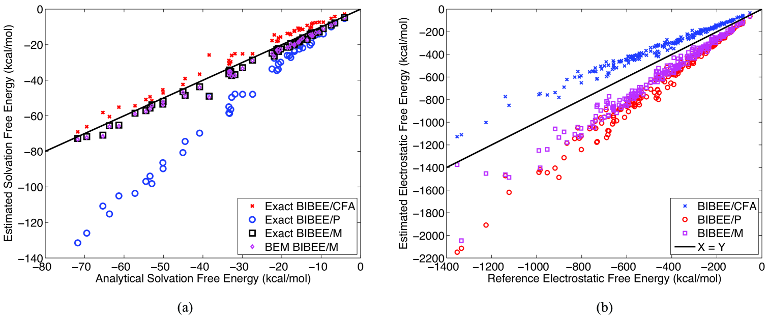
Figure 2: Modifying BIBEE using BIBEE/CFA for the monopole moment and BIBEE/P provides a tighter lower bound for charged molecules. (a) Correlation plot of the BIBEE estimated electrostatic solvation free energies, for multiple sets of 25 randomly located point charges in a sphere of radius 5 Å, with dielectric constants $\epsilon_{1}=4$ and $\epsilon_{2}=80$. Results labeled BEM BIBEE/M illustrate the same model computed using the BEM implementation of BIBEE, i.e. a numerical method suitable for arbitrary geometries. (b) Correlation plot of the improved BIBEE estimates for electrostatic solvation free energies for 200 proteins from the test set of Feig et al [21], using CHARMM22 radii and charges and dielectric constants $\epsilon_{1}=4$ and $\epsilon_{2}=80$.

Table 1: Dependence of modified BIBEE model accuracy on the eigenvalue approximation, taken over 50 structures from the test set of Feig et al. [21]. See main text for calculation details.

$\lambda$	-0.10	-0.14	-0.16	-0.18	-0.20	-0.22
RMSD (kcal/mol)	67.4	40.5	29.4	21.0	18.1	21.9
Mean deviation (%)	12.5	7.4	5.3	4.1	3.6	4.3

We then used the single fit parameter $\lambda=-0.20$ to estimate the electrostatic solvation free energies for the 610 proteins in the Feig et al. test set (Figure 4); the RMSD of the modified approach was 22.9 kcal/mol (3.2% mean deviation), illustrating that a simple one-parameter model is capable of excellent accuracy on a wide range of protein sizes and shapes. For a simple example of the model’s capability to capture energetic differences as a function of conformation, and also to illustrate the model’s performance compared to a modern GB theory, we employ 50 structures of the peptide met-enkephalin taken from all-atom molecular dynamics in explicit solvent, which were generated in earlier work [6]. Figure 5 contains plots of the numerically calculated free energies, as well as those computed using the GBMV module of CHARMM [11]. The $\lambda=-0.20$ approximation is clearly a significant improvement over the original BIBEE/CFA and BIBEE/P estimates, but further from the actual numerical result than GBMV; the RMSD for GBMV is 1.41 kcal/mol. However, if one first determines $\lambda$ so that the modified BIBEE matches the numerical result at the first snapshot (labeled $t=0$), then the modified BIBEE is competitive with GBMV in accuracy (1.88 kcal/mol). This suggests that pre-computation of appropriate fitting parameters, when rigorous approaches are found for their derivation, may enable BIBEE methods to be suitable for calculating averages as found in MM/PBSA computations[14].

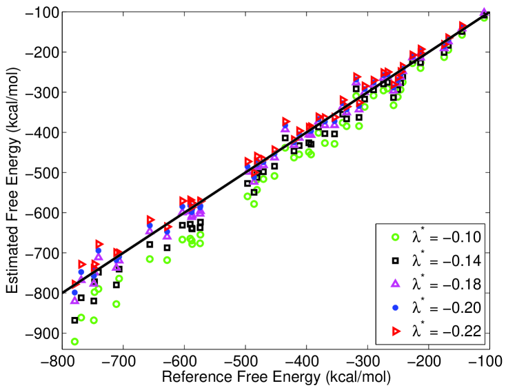
Figure 3: Dependence of modified BIBEE model accuracy on the eigenvalue approximation, taken over 50 structures from the test set of Feig et al. [21] using CHARMM22 radii and charges and dielectric constants $\epsilon_{1}=4$ and $\epsilon_{2}=80$.

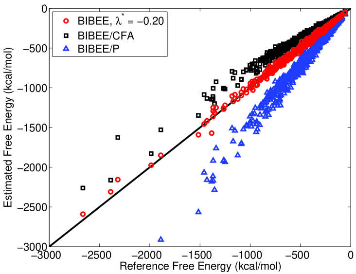
Figure 4: Electrostatic solvation free energies for all of the proteins from the test set of Feig et al. [21], using CHARMM22 radii and charges and dielectric constants $\epsilon_{1}=4$ and $\epsilon_{2}=80$, the original BIBEE/CFA and BIBEE/P models, as well as the modified BIBEE with the eigenvalue approximation $\lambda=-0.20$.

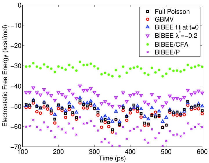
Figure 5: Electrostatic solvation free energies for 50 structures of met-enkephalin taken from an all-atom molecular dynamics simulation in explicit water. The GBMV results were calculated using CHARMM [11] and the remainder were calculated using $\epsilon_{1}=1$, $\epsilon_{2}=80$, and CHARMM22 radii and charges. See text for other calculation details.

6 Discussion

In this paper, we have derived a complete analytical characterization of the BIBEE approximation of Poisson electrostatics for charges in spherical cavities. The simplified analysis clarifies several features of the BIBEE model, highlights an important commonality between Generalized Born models and BIBEE, and suggests an immediate correction scheme, BIBEE/M, with improved accuracy. Future work will focus on developing further mathematically rigorous improvements with clear physical interpretation. We emphasize that the BIBEE/M model possesses the same attractive characteristics as the earlier BIBEE methods, including the excellent preservation of reaction-potential eigenfunctions for non-trivial geometries.

As may be expected from the initial derivation of the BIBEE model [5], the BIBEE and GB methods share a key feature in their approximations: both approaches estimate the electrostatic solvation free energy using separation of geometric and material variables. In both approaches, the approximate free energy is calculated as the product of two quantities, one purely a function of the dielectric constants, and the other quantity, which is solely a function of the geometry: dielectric boundary and charge distribution. For the initial GB/CFA models, this quantity combined the effective Born radii and the Still equation; for the BIBEE models, it relates to the Coulomb potential operators. Deviations from separability have been recognized and analyzed in detail by Onufriev and collaborators [59, 58]. In our work, we are exploring how far a purely mathematical framework may go to develop an acceptably accurate approximation to the continuum electrostatic problem, that is, before one invokes approximations specific to biomolecular simulations, such as the Still equation.

We have shown that for spherical geometries, the eigenfunctions of the approximate reaction-potential operator are exact, a result that can easily be shown to hold also for planar half-space problems. Remarkably, the proof for spheres does not rely on the spectral properties of the boundary-integral operators employed in proving that BIBEE/CFA is a rigorous upper bound to the actual Poisson free energy [6]. The eigenvector analysis can and should be analyzed from this perspective also, which may furnish additional insights into the BIBEE approximation. In particular, for the sphere it can be shown that the single-layer integral operator and the normal electric field operator are related by a simple scale factor; thus, for the sphere the operators share eigenvectors, and the normal electric field is symmetric—which is not true for general surfaces. Further rigorous improvements may be possible for nonspherical problems if operator analysis reveals the relative importance of these properties in determining the accuracy of the BIBEE eigenvectors.

The BIBEE/M analytical correction for the dominant mode described in Section 4 is not as easily extended to higher modes, unfortunately, because the surface electric fields for the higher modes are geometry dependent. Using a nonzero $\lambda$ for the other modes provides good accuracy on a range of problems, and if fit for a particular protein can rival GBMV on certain tests, but it is naturally preferable to design approximations that can be systematically improved. In future work, we will explore how the dominant eigenvectors and eigenvalues of the integral operator may be approximated to provide improved accuracy.

References

- [1] M. D. Altman, J. P. Bardhan, B. Tidor, and J. K. White. FFTSVD: A fast multiscale boundary-element method solver suitable for BioMEMS and biomolecule simulation. IEEE T. Comput.-Aid. D., 25:274–284, 2006.
- [2] M. D. Altman, J. P. Bardhan, J. K. White, and B. Tidor. Accurate solution of multi-region continuum electrostatic problems using the linearized Poisson–Boltzmann equation and curved boundary elements. J. Comput. Chem., 30:132–153, 2009.
- [3] N. A. Baker. Improving implicit solvent simulations: A Poisson-centric view. Curr. Opin. Struc. Biol., 15:137–143, 2005.
- [4] N. A. Baker, D. Sept, M. J. Holst, and J. A. McCammon. Electrostatics of nanoysystems: Application to microtubules and the ribosome. Proc. Natl. Acad. Sci. USA, 98:10037–10041, 2001.
- [5] J. P. Bardhan. Interpreting the Coulomb-field approximation for Generalized-Born electrostatics using boundary-integral equation theory. J. Chem. Phys., 129(144105), 2008.
- [6] J. P. Bardhan, M. G. Knepley, and M. Anitescu. Bounding the electrostatic free energies associated with linear continuum models of molecular solvation. J. Chem. Phys., 130:104108, 2009.
- [7] D. Bashford and D. A. Case. Generalized Born models of macromolecular solvation effects. Annu. Rev. Phys. Chem., 51:129–152, 2000.
- [8] D. Boda, D. Gillespie, W. Nonner, D. Henderson, and B. Eisenberg. Computing induced charges in inhomogeneous dielectric media: Application in a Monte Carlo simulation of complex ionic systems. Phys. Rev. E, 69:046702, 2004.
- [9] A. J. Bordner and G. A. Huber. Boundary element solution of the linear Poisson–Boltzmann equation and a multipole method for the rapid calculation of forces on macromolecules in solution. J. Comput. Chem., 24:353–367, 2003.
- [10] A. H. Boschitsch, M. O. Fenley, and H.-X. Zhou. Fast boundary element method for the linear Poisson–Boltzmann equation. J. Phys. Chem. B, 106(10):2741–54, 2002.
- [11] B. R. Brooks, R. E. Bruccoleri, B. D. Olafson, D. J. States, S. Swaminathan, and M. Karplus. CHARMM: A program for macromolecular energy, minimization, and dynamics calculations. J. Comput. Chem., 4:187–217, 1983.
- [12] Q. Cai, M.-J. Hsieh, J. Wang, and R. Luo. Performance of nonlinear finite-diference Poisson–Boltzmann solvers. J. Chem. Theory Comput., 6:203–211, 2010.
- [13] E. Cances, B. Mennucci, and J. Tomasi. A new integral equation formalism for the polarizable continuum model: Theoretical background and applications to isotropic and anisotropic dielectrics. J. Chem. Phys., 107(8):3032–3041, 1997.
- [14] N. Carrascal and D. F. Green. Energetic decomposition with the Generalized-Born and Poisson–Boltzmann solvent models: Lessons from association of G-protein components. J. Phys. Chem. B, 114:5096–5116, 2010.
- [15] D. A. Case, T. E. Cheatham III, T. Darden, H. Gohlke, R. Luo, K. M. Merz Jr., A. Onufriev, C. Simmerling, B. Wang, and R. J. Woods. The Amber biomolecular simulations programs. J. Comput. Chem., 26:1668–1688, 2005.
- [16] D. Chen, Z. Chen, C. Chen, W. Geng, and G.-W. Wei. MIBPB: A software package for electrostatic analysis. J. Comput. Chem., 2010.
- [17] C. M. Cortis and R. A. Friesner. Numerical solution of the Poisson–Boltzmann equation using tetrahedral finite-element meshes. J. Comput. Chem., 18:1591–1608, 1997.
- [18] C. J. Cramer and D. G. Truhlar. Implicit solvation models: Equilibria, structure, spectra, and dynamics. Chem. Rev., 99:2161–2200, 1999.
- [19] B. N. Dominy and C. L. Brooks III. Development of a generalized Born model parametrization for proteins and nucleic acids. J. Phys. Chem. B, 103:3765–3773, 1999.
- [20] M. Feig, J. Chocholous̆ová, and S. Tanizaki. Extending the horizon: Towards the efficient modeling of large biomolecular complexes in atomic detail. Theor. Chem. Acc., 116:194–205, 2006.
- [21] M. Feig, A. Onufriev, M. S. Lee, W. Im, D. A. Case, and C. L. Brooks III. Performance comparison of generalized Born and Poisson methods in the calculation of electrostatic solvation energies for protein structures. J. Comput. Chem., 25:265–284, 2004.
- [22] A. Ghosh, C. S. Rapp, and R. A. Friesner. Generalized Born model based on a surface integral formulation. J. Phys. Chem. B, 102:10983–10990, 1998.
- [23] M. K. Gilson and B. Honig. Calculation of the total electrostatic energy of a macromolecular system: Solvation energies, binding energies, and conformational analysis. Proteins, 4:7–18, 1988.
- [24] M. K. Gilson, A. Rashin, R. Fine, and B. Honig. On the calculation of electrostatic interactions in proteins. J. Mol. Biol., 184:503–516, 1985.
- [25] T. Grycuk. Deficiency of the Coulomb-field approximation in the generalized Born model: An improved formula for Born radii evaluation. J. Chem. Phys., 119(9):4817–4826, 2003.
- [26] P. B. Harbury, J. J. Plecs, B. Tidor, T. Alber, and P. S. Kim. High-resolution protein design with backbone freedom. Science, 282:1462–1467, 1998.
- [27] D. Horvath, D. vanBelle, G. Lippens, and S. J. Wodak. Development and parametrization of continuum solvent models. I. Models based on the boundary element method. J. Chem. Phys., 104:6679–6695, 1996.
- [28] J. D. Jackson. Classical Electrodynamics. Wiley, 3rd edition, 1998.
- [29] A. Jean-Charles, A. Nicholls, K. Sharp, B. Honig, A. Tempczyk, T. F. Hendrickson, and W. C. Still. Electrostatic contributions to solvation energies: Comparison of free energy perturbation and continuum calculations. J. Am. Chem. Soc., 113:1454–1455, 1991.
- [30] A. D. MacKerell Jr., D. Bashford, M. Bellott, R. L. Dunbrack Jr., J. D. Evanseck, M. J. Field, S. Fischer, J. Gao, H. Guo, S. Ha, D. Joseph–McCarthy, L. Kuchnir, K. Kuczera, F. T. K. Lau, C. Mattos, S. Michnick, T. Ngo, D. T. Nguyen, B. Prodhom, W. E. Reiher III, B. Roux, M. Schlenkrich, J. C. Smith, R. Stote, J. Straub, M. Watanabe, J. Wiorkiewicz–Kuczera, D. Yin, and M. Karplus. All-atom empirical potential for molecular modeling and dynamics studies of proteins. J. Phys. Chem. B, 102:3586–3616, 1998.
- [31] A. H. Juffer, E. F. F. Botta, B. A. M. van Keulen, A. van der Ploeg, and H. J. C. Berendsen. The electric potential of a macromolecule in a solvent: A fundamental approach. J. Comput. Phys., 97(1):144–171, 1991.
- [32] J. G. Kirkwood. Theory of solutions of molecules containing widely separated charges with special application to zwitterions. J. Chem. Phys., 2:351, 1934.
- [33] I. Klapper, R. Hagstrom, R. Fine, K. Sharp, and B. Honig. Focusing of electric fields in the active site of Cu-Zn superoxide dismutase: Effects of ionic strength and amino-acid modification. Proteins, 1:47–59, 1986.
- [34] M. S. Lee, F. R. Salsbury, and C. L. Brooks III. Novel generalized Born methods. J. Chem. Phys., 116(24):10606–10604, 2002.
- [35] J. Liang and S. Subramaniam. Computation of molecular electrostatics with boundary element methods. Biophys. J., 73(4):1830–1841, 1997.
- [36] H.-Y. Liu, S. Z. Grinter, and X. Zou. Multiscale generalized Born modeling of ligand binding energies for virtual database screening. J. Phys. Chem. B, 113:11793–11799, 2009.
- [37] B. Z. Lu, X. L. Cheng, J. Huang, and J. A. McCammon. Order N algorithm for computation of electrostatic interactions in biomolecular systems. Proc. Natl. Acad. Sci. USA, 103(51):19314–19319, 2006.
- [38] B. Z. Lu, D. Q. Zhang, and J. A. McCammon. Computation of electrostatic forces between solvated molecules determined by the Poisson–Boltzmann equation using a boundary element method. J. Chem. Phys., 122, 2005.
- [39] J. Michel, R. D. Taylor, and J. W. Essex. The parameterization and validation of generalized Born models using the pairwise descreening approximation. J. Comput. Chem., 25:1760–1770, 2004.
- [40] S. Miertus, E. Scrocco, and J. Tomasi. Electrostatic interactions of a solute with a continuum – a direct utilization of ab initio molecular potentials for the prevision of solvent effects. Chem. Phys., 55(1):117–129, 1981.
- [41] J. Mongan, C. Simmerling, J. A. McCammon, D. A. Case, and A. Onufriev. Generalized Born model with a simple, robust molecular volume correction. J. Chem. Theory Comput., 3:156–169, 2007.
- [42] J. Mongan, W. A. Svrcek-Seiler, and A. Onufriev. Analysis of integral expressions for effective Born radii. J. Chem. Phys., 127(185101), 2007.
- [43] A. Nicholls and B. Honig. A rapid finite-difference algorithm, utilizing successive over-relaxation to solve the Poisson–Boltzmann equation. J. Comput. Chem., 12:435–445, 1991.
- [44] A. Onufriev, D. Bashford, and D. A. Case. Modification of the generalized Born model suitable for macromolecules. J. Phys. Chem. B, 104(15):3712–3720, 2000.
- [45] A. Onufriev, D. A. Case, and D. Bashford. Effective Born radii in the generalized Born approximation: The importance of being perfect. J. Comput. Chem., 23:1297–1304, 2002.
- [46] J. C. Phillips, R. Braun, W. Wang, J. Gumbart, E. Tajkhorshid, E. Villa, C. Chipot, R. D. Skeel, L. Kale, and K. Schulten. Scalable molecular dynamics with NAMD. J. Comput. Chem., 26:1781–1802, 2005.
- [47] E. O. Purisima and S. H. Nilar. A simple yet accurate boundary-element method for continuum dielectric calculations. J. Comput. Chem., 16(6):681–689, 1995.
- [48] D. Qiu, P. S. Shenkin, F. P. Hollinger, and W. C. Still. The GB/SA continuum model for solvation. A fast analytical method for the calculation of approximate Born radii. J. Phys. Chem. A, 101(16):3005–3014, 1997.
- [49] S. W. Rick and B. J. Berne. The aqueous solvation of water: A comparison of continuum methods with molecular dynamics. J. Am. Chem. Soc., 116:3949–3954, 1994.
- [50] S. Ritter. A sum-property of the eigenvalues of the electrostatic integral operator. J. Math. Anal. Appl., 196:120–134, 1995.
- [51] A. N. Romanov, S. N. Jabin, Y. B. Martynov, A. V. Sulimov, F. V. Grigoriev, and V. B. Sulimov. Surface generalized Born method: A simple, fast, and precise implicit solvent model beyond the Coulomb approximation. J. Phys. Chem. A, 108(43):9323–9327, 2004.
- [52] B. Roux and T. Simonson. Implicit solvent models. Biophys. Chem., 78:1–20, 1999.
- [53] S. Rush, A. H. Turner, and A. H. Cherin. Computer solution for time-invariant electric fields. J. Appl. Phys., 37(6):2211–2217, 1966.
- [54] M. Sanner, A. J. Olson, and J. C. Spehner. Reduced surface: An efficient way to compute molecular surfaces. Biopolymers, 38:305–320, 1996.
- [55] M. Schaefer and M. Karplus. A comprehensive analytical treatment of continuum electrostatics. J. Phys. Chem., 100:1578–1599, 1996.
- [56] K. A. Sharp and B. Honig. Electrostatic interactions in macromolecules: Theory and applications. Annu. Rev. Biophys. Bio., 19:301–332, 1990.
- [57] P. B. Shaw. Theory of the Poisson Green’s-function for discontinuous dielectric media with an application to protein biophysics. Phys. Rev. A, 32(4):2476–2487, 1985.
- [58] G. Sigalov, A. Fenley, and A. Onufriev. Analytical electrostatics for biomolecules: Beyond the generalized Born approximation. J. Chem. Phys., 124(124902), 2006.
- [59] G. Sigalov, P. Scheffel, and A. Onufriev. Incorporating variable dielectric environments into the generalized Born model. J. Chem. Phys., 122:094511, 2005.
- [60] T. Simonson. Macromolecular electrostatics: Continuum models and their growing pains. Curr. Opin. Struc. Biol., 11:243–252, 2001.
- [61] W.C. Still, A. Tempczyk, R. C. Hawley, and T. F. Hendrickson. Semianalytical treatment of solvation for molecular mechanics and dynamics. J. Am. Chem. Soc., 112(16):6127–6129, 1990.
- [62] C. Tanford and J. G. Kirkwood. Theory of protein titration curves I. General equations for impenetrable spheres. J. Am. Chem. Soc., 59:5333–5339, 1957.
- [63] H. Tjong and H.-X. Zhou. GBr6: A parameterization-free, accurate, analytical generalized Born method. J. Phys. Chem. B, 111:3055–3061, 2007.
- [64] C. L. Vizcarra and S. L. Mayo. Electrostatics in computational protein design. Curr. Opin. Chem. Biol., 9:622–626, 2005.
- [65] Y. N. Vorobjev, J. A. Grant, and H. A. Scheraga. A combined iterative and boundary element approach for solution of the nonlinear Poisson–Boltzmann equation. J. Am. Chem. Soc., 114:3189–3196, 1992.
- [66] A. Warshel and S. T. Russell. Calculations of electrostatic interactions in biological systems and in solutions. Quart. Rev. Biophys., 17:283–422, 1984.
- [67] J. Warwicker and H. C. Watson. Calculation of the electric potential in the active site cleft due to alpha-helix dipoles. J. Mol. Biol., 157:671–679, 1982.
- [68] B. J. Yoon and A. M. Lenhoff. A boundary element method for molecular electrostatics with electrolyte effects. J. Comput. Chem., 11(9):1080–1086, 1990.
- [69] T. J. You and S. C. Harvey. Finite-element approach to the electrostatics of macromolecules with arbitrary geometries. J. Comput. Chem., 14:484–501, 1993.
- [70] S. N. Yu, Y. C. Zhou, and G. W. Wei. Matched interface and boundary (MIB) method for elliptic problems with sharp-edged interfaces. J. Comput. Phys., 224(2):729–756, 2007.
- [71] R. J. Zauhar and R. S. Morgan. A new method for computing the macromolecular electric-potential. J. Mol. Biol., 186:815–820, 1985.
- [72] H. X. Zhou. Boundary-element solution of macromolecular electrostatics - interaction energy between 2 proteins. Biophys. J., 65:955–963, 1993.